
CHAPTER 2
Fixed Income – Strategic Asset Allocation
Overview
This chapter undertakes a detailed examination of the return properties of fixed income securities. We start with an additive decomposition of total returns into “rates” and “spread” components. The influence of interest rates on fixed income securities is large and it pervades all fixed income securities. We will see the importance of rates declines when there is greater risk of nonpayment of the cash flows. This helps us structure our thinking for later chapters when we build a framework to forecast returns of fixed income securities: Exactly what component of returns should we focus on? We will then document the variety of betas (traditional market risk premia) that are commonly accessible in fixed income markets and show how they help diversify in the context of strategic asset allocation decisions. We will explain how and why fixed income allocations should be a core part of asset owner portfolios. This will involve a detailed discussion of yields and determinants of yields, setting up the stage for our next chapter on tactical allocations within fixed income.
2.1 WHAT ARE THE KEY DRIVERS OF FIXED INCOME SECURITY RETURNS?
In Chapter 1 we introduced the terms yield and duration. We will now turn to utilizing these measures to decompose the total returns to fixed income securities. We will start with the Bloomberg Global Aggregate Index and we will decompose the total returns of the Global Treasury, Global Government Related, Global Corporate, and Global Securitized subsectors within the Global Aggregate Index. We will also look at the total returns of the Bloomberg Global High Yield Index and the Bloomberg Emerging Market USD Aggregate Index. This will give us the opportunity to look at a broad set of fixed income securities where there is considerable variation in the credit risk (i.e., possibility of nonpayment of cash flows) of issuers.
We will start with total returns for each category of issuers. Exhibit 2.1 shows the arithmetic annualized average returns and standard deviations for the six respective categories for the 2000–2020 period. The categories are sorted based on increasing credit risk, hence Global High Yield (GHY) is to the right. Return realizations are sample period dependent, so we are not going to emphasize the average returns too much for this single 20‐year period. That said, risk‐adjusted returns (as indicated by the Sharpe ratio, which is the ratio of the annualized average returns to the annualized standard deviation of returns) are very impressive. The purpose here is to understand the importance of components of returns.
EXHIBIT 2.1 Total returns (annualized averages and standard deviation) for Global Treasury, Global Government Related, Global Securitized, Global Corporates, Emerging Market USD Aggregate, and Global High Yield indices. Returns are excess of cash (US T‐Bills).
| TSY | GREL | SEC | CORP | EM‐USD | GHY | |
|---|---|---|---|---|---|---|
| Average | 4.59 | 4.71 | 4.47 | 5.52 | 6.94 | 7.06 |
| Std. Dev. | 6.49 | 5.41 | 3.33 | 6.49 | 9.02 | 10.14 |
| Sharpe ratio | 0.71 | 0.87 | 1.34 | 0.85 | 0.77 | 0.70 |
Source: Bloomberg Indices.
Our next step is to decompose total returns into a component attributable to movements in yields (let's call this the “rates” portion, ![]() ) and a residual component that captures everything else such as liquidity risk and spread risk (let's call this the “spread” portion,
) and a residual component that captures everything else such as liquidity risk and spread risk (let's call this the “spread” portion, ![]() ). We will first quantify
). We will first quantify ![]() . An easy way to conceptualize the rates component of returns is to think of “duration.” When yields move by a certain amount, multiplying that yield change by –1 × duration will give an approximation of the rates component of returns. As discussed in Chapter 1, this is an approximation, because it assumes a uniform change in yields (discount rates) across all bond cash flows that need to be discounted. More generally, duration can be measured at multiple tenor points. This gives rise to a term structure of duration measures also referred to as key rate durations (with the “key” reflecting standard tenor points such as six‐month, one‐year, two‐years, etc.). Each bond will be assigned a set of key rate‐duration exposures. For a given unit of time (e.g., a month) you can then observe yield changes at each key point and the sum product of the key rate durations, with the yield changes at each key point providing a measure of
. An easy way to conceptualize the rates component of returns is to think of “duration.” When yields move by a certain amount, multiplying that yield change by –1 × duration will give an approximation of the rates component of returns. As discussed in Chapter 1, this is an approximation, because it assumes a uniform change in yields (discount rates) across all bond cash flows that need to be discounted. More generally, duration can be measured at multiple tenor points. This gives rise to a term structure of duration measures also referred to as key rate durations (with the “key” reflecting standard tenor points such as six‐month, one‐year, two‐years, etc.). Each bond will be assigned a set of key rate‐duration exposures. For a given unit of time (e.g., a month) you can then observe yield changes at each key point and the sum product of the key rate durations, with the yield changes at each key point providing a measure of ![]() (i.e., a duration‐weighted average effect of yield changes). A given portfolio does not have the same rate return as a basket of government bonds; that is only true if their duration is the same. For example, the rates components of returns for the various fixed income asset classes in Exhibit 2.1 are not constant, in part due to differences in duration. The difference between total returns and the rates component is then the “spread” component of returns. As Asvanunt and Richardson (2017) note, simply subtracting treasury returns is incorrect, as it assumes duration is identical between the bonds in the portfolio whose returns are to be decomposed and the government bonds in the treasury portfolio. The simple additive total return decomposition is as follows:
(i.e., a duration‐weighted average effect of yield changes). A given portfolio does not have the same rate return as a basket of government bonds; that is only true if their duration is the same. For example, the rates components of returns for the various fixed income asset classes in Exhibit 2.1 are not constant, in part due to differences in duration. The difference between total returns and the rates component is then the “spread” component of returns. As Asvanunt and Richardson (2017) note, simply subtracting treasury returns is incorrect, as it assumes duration is identical between the bonds in the portfolio whose returns are to be decomposed and the government bonds in the treasury portfolio. The simple additive total return decomposition is as follows:
An alternative, but conceptually equivalent, approach to decomposing returns is to match the cash flow profiles of a given risky bond with a riskless bond. The returns on the cash‐flow‐matched riskless bond is then ![]() , and as per Equation 2.1, the difference between the total return on the risky bond and
, and as per Equation 2.1, the difference between the total return on the risky bond and ![]() is
is ![]() . These measures are typically computed by index providers and are readily available to market participants.
. These measures are typically computed by index providers and are readily available to market participants.
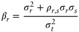
Exhibit 2.2 reports the contribution of ![]() and
and ![]() for our six fixed income categories. To ease comparison of the relative contribution of return components across categories, total returns are standardized to 100 percent. Over this period, there has been a very attractive risk‐adjusted return to riskless government bonds. Exhibit 2.1 showed a Sharpe ratio of 0.71 for global government bonds, and all of that return is attributable to “rates” (by definition). The tailwind of generally declining interest rates and yields over the 2000–2020 period is a key source of the strong positive returns to fixed income assets across the board. Across the other five categories we see that average returns over this period are dominated by the rates component and notably that the importance of the rates component declines as we move from left to right consistent with the increasing importance of credit, or default risk, as we move from safe developed sovereign issuers to risky corporate and emerging market issuers.
for our six fixed income categories. To ease comparison of the relative contribution of return components across categories, total returns are standardized to 100 percent. Over this period, there has been a very attractive risk‐adjusted return to riskless government bonds. Exhibit 2.1 showed a Sharpe ratio of 0.71 for global government bonds, and all of that return is attributable to “rates” (by definition). The tailwind of generally declining interest rates and yields over the 2000–2020 period is a key source of the strong positive returns to fixed income assets across the board. Across the other five categories we see that average returns over this period are dominated by the rates component and notably that the importance of the rates component declines as we move from left to right consistent with the increasing importance of credit, or default risk, as we move from safe developed sovereign issuers to risky corporate and emerging market issuers.
When we explore investment frameworks for government bonds, corporate bonds, and emerging market USD bonds later in this book, we will be focusing on the portion of return that is unique to that respective fixed income category. For (developed market) government bonds the return source is completely attributable to yields (rates). Hence our investment focus needs to be centered on where yields are today and where they are likely to move to in the future. For corporate bonds, we will focus our investment effort on the potential for credit excess returns. Of course, corporate bonds inherit exposures to yields, but this is not why we trade corporate bonds. As we will see later, corporate bonds are a costly asset class to trade, so why pay a lot to express investment views on yields when you can do so far more cheaply with government bonds directly. For emerging market USD bonds, we will also focus our investment attention on the potential for spread returns unique to that market, again for the same reasons.

EXHIBIT 2.2 Total return decomposition into “rates” and “spread” components for Global Treasury, Global Government Related, Global Securitized, Global Corporates, Emerging Market USD Aggregate, and Global High Yield indices.
Source: Data from Bloomberg Indices.
In addition to decomposing total returns, we can also decompose the variation of total returns for fixed income securities. A simple way to do this is to compute the standard deviation of ![]() and
and ![]() over the 2000–2020 period for each of our six fixed income categories. Exhibit 2.3 shows the relative contribution of the two sources of return standard deviation.
over the 2000–2020 period for each of our six fixed income categories. Exhibit 2.3 shows the relative contribution of the two sources of return standard deviation.
We see a similar pattern in the return variation decomposition as we saw with the return decomposition itself. The importance of the rates component declines as we move from left to right consistent with the increasing importance of credit, or default risk, as we move from safe developed sovereign issuers to risky corporate and emerging market issuers. Exhibit 2.3 is an imprecise method to show the relative importance of components of returns to explain the temporal variation in returns. The imprecision is due to correlation. The components of returns, ![]() and
and ![]() , are correlated, and over the 2000–2020 period they are typically negatively correlated, especially for those fixed income securities with heightened credit risk. This is related to the topic of stock–bond correlation that we will cover later in this chapter. The correlation of the spread component and rates component of returns for the Global Securitized and Global Corporate subindices are –0.10 and –0.07, respectively. In contrast, the correlation of the spread component and rates component of returns for the Emerging Market USD Aggregate and Global High Yield indices are –0.37 and –0.35, respectively. This is a direct manifestation of the strong negative association between stocks and bonds that has been seen over the past two decades. Fixed income securities with significant credit risk share a very high positive correlation with equity securities.
, are correlated, and over the 2000–2020 period they are typically negatively correlated, especially for those fixed income securities with heightened credit risk. This is related to the topic of stock–bond correlation that we will cover later in this chapter. The correlation of the spread component and rates component of returns for the Global Securitized and Global Corporate subindices are –0.10 and –0.07, respectively. In contrast, the correlation of the spread component and rates component of returns for the Emerging Market USD Aggregate and Global High Yield indices are –0.37 and –0.35, respectively. This is a direct manifestation of the strong negative association between stocks and bonds that has been seen over the past two decades. Fixed income securities with significant credit risk share a very high positive correlation with equity securities.
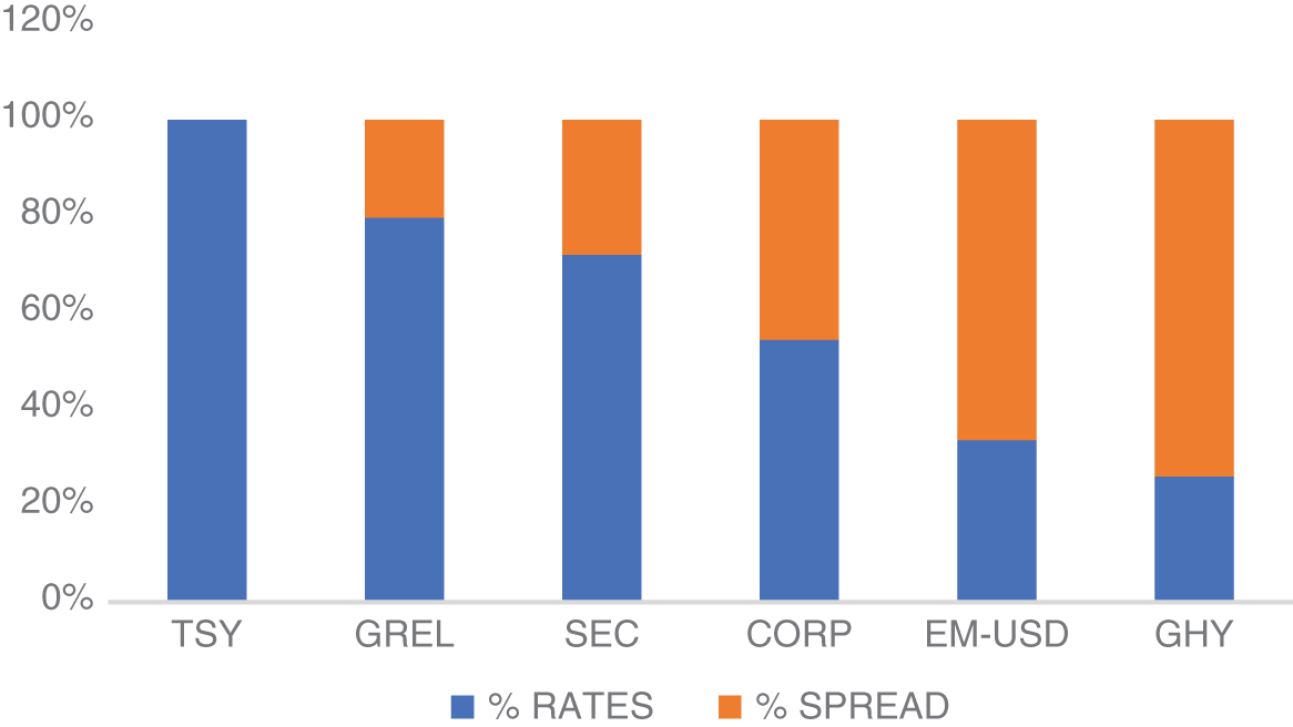
EXHIBIT 2.3 Standard deviation contribution of “rates” and “spread” return components for Global Treasury, Global Government Related, Global Securitized, Global Corporates, Emerging Market USD Aggregate, and Global High Yield indices.
Source: Data from Bloomberg Indices.
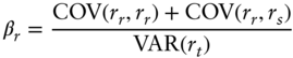
To account for the correlation across return subcomponents, we need to introduce some terminology for variance and covariance. We can rewrite Equation 2.1 using symbols for the various types of returns we have discussed so far: (i) ![]() for total returns, (ii)
for total returns, (ii) ![]() for the rates component of returns, and (iii)
for the rates component of returns, and (iii) ![]() for the spread component of returns.
for the spread component of returns.
Using the variance operator (![]() is the standard deviation of
is the standard deviation of ![]() , and
, and ![]() is the correlation between
is the correlation between ![]() and
and ![]() ), we have:
), we have:
If we divide this expression by total return variance, ![]() , we arrive at an additive decomposition of return variation:
, we arrive at an additive decomposition of return variation:

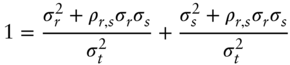
How correlation affects return variation decomposition should now be clear(er). The covariance between the rate and spread portion of returns is explicitly accounted for. These components are not perfectly correlated with each other and, as mentioned earlier, can be negatively correlated to each other. This results in a meaningful lower variation for total returns than the simple sum of return variation across the two components. That's diversification for you.
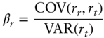
Although you could estimate volatilities and correlations of the various components of returns, there is a simpler approach that makes use of linear algebra. We can run the following simple regressions, and the regression coefficients provide our answer.
The regression coefficients contain the relevant information:

We can combine Equation (2.2) with Equation (2.8) and expand some terms:
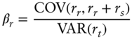
And similarly, for the spread portion of returns:
Now it is easy to see that ![]() , and the respective betas are the exact same calculations as in Equation (2.5). Exhibit 2.4 shows the total return variance decomposition using this approach.
, and the respective betas are the exact same calculations as in Equation (2.5). Exhibit 2.4 shows the total return variance decomposition using this approach.
EXHIBIT 2.4 Total return variance decomposition into “rates” and “spread” component for Global Treasury, Global Government Related, Global Securitized, Global Corporates, Emerging Market USD Aggregate, and Global High Yield indices.
Source: Data from Bloomberg Indices.
The difference between Exhibit 2.3 and Exhibit 2.4 is simply the correlation between return components. For those fixed income assets with greater risk, and hence greater correlation to equity securities, the importance of rates is greatly reduced. This is the effect of the greater negative correlation between the rate and spread component of returns for those types of assets.
2.2 WHAT TRADITIONAL RISK PREMIA CAN BE HARVESTED IN FIXED INCOME?
Now that we have an appreciation of the source of returns from fixed income securities, let's ask a fundamental question: What unique return sources are available to asset owners in fixed income? We will answer that question looking at a broad set of fixed income returns across the following categories: (i) Global Treasury (same index as previously), (ii) Emerging Market Local Currency Government, (iii) US Mortgage Backed Securities (a subset of the Global Securitized subindex examined previously), (iv) Corporate (global Investment‐Grade corporate bonds), (v) Emerging Market USD Aggregate, (vi), US High Yield (as subset of the Global High Yield we examined previously), and (vii) US Leveraged Loans (using Credit Suisse Leveraged Loan Total Return). We will also look at global equity market returns (MSCI World Index). Returns data for categories (i)–(vi) are sourced from Bloomberg Indices. All return series are measured monthly and reported in USD.
Exhibit 2.5 reports the correlations across these return series using the longest possible time series for each category available. The first row in Exhibit 2.5 lists the first year data is available for each series. These correlations are all based on total returns, which we now know share a large common rates component across the fixed income categories. Therefore, it is not surprising to see reasonably high correlations across the various categories using total returns (inclusive of cash returns). And these correlations are computed over the longest time series possible for each pair, so these averages will mask any temporal variation.
There are a couple of notable patterns. The riskier fixed income securities have higher correlations to each other (e.g., Emerging Market bonds, corporate bonds, and loans), and to equity markets. A cleaner way to assess the potential uniqueness for each source of returns is to look at excess returns. For the credit sensitive assets (corporate bonds, loans, and emerging market debt) we remove the rates component of returns as discussed earlier (i.e., accounting for the duration exposure to interest rates). For government bonds and equities, we subtract one‐month US Treasury Bill returns (cash returns) to compute excess returns for those categories. Exhibit 2.6 reports the correlations across monthly excess returns for the same categories (the time periods are shorter for some categories due to the requirement of analytics for subtracting the rate component of returns).
EXHIBIT 2.5 Correlations of USD monthly total returns across Global Treasury, Emerging Market Local Currency, US Mortgage‐Backed Securities, Investment Grade Corporates, Emerging Market USD debt, Corporate High Yield Bonds, Leveraged Loans, and MSCI World Equity.
| 1987 | 2008 | 1976 | 1973 | 2001 | 1983 | 1992 | 1970 | |
|---|---|---|---|---|---|---|---|---|
| GL TSY | EM LOCAL | US MBS | CORP IG | EM USD | CORP HY | LOANS | WORLD EQ | |
| GL TSY | 1.00 | 0.66 | 0.52 | 0.55 | 0.48 | 0.13 | −0.04 | 0.20 |
| EM LOCAL | 1.00 | 0.18 | 0.57 | 0.78 | 0.67 | 0.42 | 0.70 | |
| US MBS | 1.00 | 0.83 | 0.33 | 0.21 | –0.13 | 0.14 | ||
| CORP IG | 1.00 | 0.72 | 0.55 | 0.37 | 0.34 | |||
| EM USD | 1.00 | 0.77 | 0.57 | 0.65 | ||||
| CORP HY | 1.00 | 0.77 | 0.61 | |||||
| LOANS | 1.00 | 0.50 | ||||||
| WORLD EQ | 1.00 |
Sources: Data from Bloomberg Indices, Credit Suisse, MSCI.
The correlation between the credit‐sensitive assets and the correlation of credit‐sensitive assets to equity markets increases when looking at excess returns. This is an important fact that will become a common theme in the book. There are categories of securities within the fixed income landscape that are strongly positive correlated with equity markets, and there are other categories of fixed income assets that have low, or even negative, correlation with stocks (e.g., government bonds over the past couple of decades). I have chosen the longest period for completeness in Exhibit 2.6 but note that more recent periods, during which the stock–bond correlation has become more negative, show even stronger positive correlations of excess returns across credit sensitive assets.
To appreciate the considerable temporal variation in the risk‐adjusted returns across fixed income sectors, Exhibit 2.7 plots rolling 36‐month Sharpe ratios, using the same measure of excess returns from Exhibit 2.6 (the astute reader will note I am a little loose with my use of the Sharpe ratio here as the excess returns are excess of cash for some return series and excess of duration for return series; a pure labeling might use the information ratio for the excess of duration return series). Although there is a clear common component across fixed income sectors (the full sample correlations in Exhibit 2.6 suggest this), there are periods when different subsectors perform better or worse than others. Let's examine what the source of this return variation might be.
EXHIBIT 2.6 Correlations of USD monthly excess returns across Global Treasury, Emerging Market Local Currency, US Mortgage‐Backed Securities, Investment Grade Corporates, Emerging Market USD debt, Corporate High Yield Bonds, Leveraged Loans, and MSCI World Equity.
| 1987 | 2008 | 1988 | 1988 | 2001 | 1988 | 1992 | 1988 | |
|---|---|---|---|---|---|---|---|---|
| GL TSY | EM LOCAL | US MBS | CORP IG | EM USD | CORP HY | LOANS | WORLD EQ | |
| GL TSY | 1.00 | 0.66 | –0.08 | 0.01 | 0.09 | –0.10 | –0.03 | 0.19 |
| EM LOCAL | 1.00 | 0.32 | 0.55 | 0.68 | 0.60 | 0.43 | 0.71 | |
| US MBS | 1.00 | 0.38 | 0.52 | 0.42 | 0.36 | 0.32 | ||
| CORP IG | 1.00 | 0.81 | 0.82 | 0.80 | 0.63 | |||
| EM USD | 1.00 | 0.85 | 0.73 | 0.75 | ||||
| CORP HY | 1.00 | 0.79 | 0.67 | |||||
| LOANS | 1.00 | 0.51 | ||||||
| WORLD EQ | 1.00 |
Sources: Data from Bloomberg Indices, Credit‐Suisse, MSCI.
But first, one caveat for the analysis in Exhibit 2.7: stale/smooth data. Certain subsectors in fixed income are notorious for their lack of liquidity, pre‐ and post‐trade price transparency, and quality of marks used in index pricing. Of the categories we have examined, corporate bonds and, especially, leveraged loans are most guilty. The Sharpe ratios are therefore overstated for these fixed‐income subcategories, because any resulting smoothing in prices and returns will dampen the empirically estimated volatilities used when computing Sharpe ratios. Yes, there are approaches to correct for staleness in pricing, but at this stage our purpose is simply to note temporal variation in performance across fixed income subsectors. This sets up our discussion on the diversifying potential of risk premia embedded in fixed income markets.
Broadly speaking we can categorize the types of fixed income risk premia as follows.
2.2.1 Term Premium (and Yields)
The term premium is the additional return an investor expects to receive from holding to maturity a long‐term risk‐free government bond relative to the return generated from rolling a series of shorter‐dated risk‐free government bonds. The risks that the longer‐term bondholder faces are not credit risk in the sense of nonpayment of coupons by the government. The risk is that price, or alternatively yield, of the long‐term government bond will change over the investment holding period, resulting in mark to market gains/losses along the way to maturity. (In contrast, the investor rolling positions across a series of shorter‐term government bonds is able to reinvest at the then‐prevailing interest rate.)

EXHIBIT 2.7 Rolling 36‐month Sharpe ratios of USD monthly excess returns across Global Treasury, Emerging Market Local Currency, US Mortgage‐Backed Securities, Investment Grade Corporates, Emerging Market USD debt, Corporate HighYield Bonds, Leveraged Loans, and MSCI World Equity.
Sources: Bloomberg Indices, Credit Suisse, MSCI.
Before we look at the returns of long‐term government bonds, let's first ensure we understand the determinants of yields on long‐term government bonds. Brooks (2021) describes a simple framework that we will lean on for our discussion. This framework is helpful to make links between yields, an indicator of return potential, and what we are talking about here: (ex‐ante) term premia.
Equation 2.14 summarizes the simple framework in Brooks (2021):
In words, the yield on a long‐term government bond is equal to the prevailing short‐term interest rates, ![]() , expectations of those same short‐term interest rates over the life of the long‐term government bond,
, expectations of those same short‐term interest rates over the life of the long‐term government bond, ![]() , and a residual component that we will call term premium. Central banks in all developed markets (our current focus) are responsible for the setting of short‐term interest rates. Although the precise mechanism can vary across countries, the idea is that the central banks influence key short‐term interest rates used by financial institutions. For example, the US Federal Reserve uses the Federal Funds Rate as its key short‐term interest rate. This is the interest rate that financial institutions charge each other for overnight lending. Although there is some disagreement about the precise role/mandate of central banks in the developed world, most market participants agree that it includes a focus on price stability and full employment. If this is the objective of the central bank, then why focus on short‐term interest rates? Central banks can control short‐term interest rates, and these rates ultimately affect the cost of borrowing for businesses and customers, leading to aggregate effects on credit and broad economic activity. This will impact employment and inflation, which are the ultimate objectives of the central bank. This is the mechanism by which modern monetary policy works (or is believed to work).
, and a residual component that we will call term premium. Central banks in all developed markets (our current focus) are responsible for the setting of short‐term interest rates. Although the precise mechanism can vary across countries, the idea is that the central banks influence key short‐term interest rates used by financial institutions. For example, the US Federal Reserve uses the Federal Funds Rate as its key short‐term interest rate. This is the interest rate that financial institutions charge each other for overnight lending. Although there is some disagreement about the precise role/mandate of central banks in the developed world, most market participants agree that it includes a focus on price stability and full employment. If this is the objective of the central bank, then why focus on short‐term interest rates? Central banks can control short‐term interest rates, and these rates ultimately affect the cost of borrowing for businesses and customers, leading to aggregate effects on credit and broad economic activity. This will impact employment and inflation, which are the ultimate objectives of the central bank. This is the mechanism by which modern monetary policy works (or is believed to work).
So with central bank objectives to target stable price and full employment, what tools do they have available to deliver on these objectives via the interest‐rate channel? Although central banks are challenged in their ability to directly control long‐term government bond yields directly (perhaps via direct market purchases), they focus on what they can influence, and here they have several options. First, as discussed earlier, they can set short‐term interest rates directly. Second, they can influence expectations of future short‐term interest rates. Via credible implementation of monetary policy over the past few decades, central banks have built up considerable trust with capital markets and are able, to a point, to signal their intentions with respect to future monetary policy decisions. Setting expectations of future short‐term interest rates is a key component of modern monetary policy. Third, central banks can directly influence the prices of financial assets by purchasing, or expressing intent to purchase, these assets in secondary markets. Central banks do not have to purchase financial assets, nor in large amounts to influence prices in large amounts; the mere expectation that they might intervene can have significant effects on prices (see e.g., Gilchrist, Wei, Yue and Zakrajsek 2021). It is this third policy tool that can influence the term premium directly.
The determinants of term premium extend far beyond central banks, because they are not the only force acting on longer‐term interest rates. There are a variety of other capital market participants and basic economic forces at work. Macroeconomic theory suggests that long‐term interest rates should be anchored to the natural real interest rate, an equilibrium concept consistent with stable inflation absent any demand and supply shocks, and long‐term inflation expectations. The role of central banks is to adjust interest rates around the natural rate based on their views of economic activity and inflation (the well‐known Taylor Rule). If central banks believe economic activity is below (above) potential, they will lower (raise) short‐term interest rates, and if they believe inflation is below (above) their target level, they will also lower (raise) interest rates. There is a risk of overemphasizing the influence of central banks on long‐term yields, as central banks respond to economic growth “gaps” and inflation “gaps.” In a free market, the long‐term anchors of yields are set by economic forces: underlying real economic growth (per capita) is the primary driver of the real rate of interest, and no central bank can wave a wand to directly change economic growth. They are responding to signals about deviations from potential growth.
Other determinants of longer‐term government bond yields that fall within the residual “term premium” include (i) uncertainty about the path of future inflation expectations (e.g., inflation uncertainty), (ii) general business cycle uncertainty can influence longer‐term government bond yields (e.g., general risk aversion), and (iii) behaviors of capital market participants such as large pools of capital (e.g., pension plans and sovereign states) whose net demand for “safe” assets can directly influence their price. Heightened concerns about inflation uncertainty would increase the term premium; heightened risk aversion in the economy would also increase the term premium. In contrast, actions from large asset owners to seek safe assets (sovereign reserve managers) or seek hedges for longer‐dated liabilities (pension funds, but perhaps their demand is more in longer‐dated corporate bonds as opposed to longer‐dated government bonds) will reduce the term premium.
In summary, there is a lot going on that influence yields on longer‐term government bonds. A component of that yield is the term premium. From an asset owner perspective, it is that term premium you are looking to capture with your allocation to government bonds. So, what does the data look like for the term premium? Rather than attempting to extract the ex‐ante term premium from yields, which is noisy at best (see e.g., Laubach and Williams 2003 and Holston, Laubach, and Williams 2017), we are going to look at ex‐post returns.
Using an updated data series from Asvanunt and Richardson (2017) covering the 1926–2020 period, we can examine the long‐run evidence from investing in long‐term government bonds relative to the alternative of short‐term government bills. The source data for this time series is Ibbotson's U.S. Long‐Term Government Bond Total Return minus Ibbotson's U.S. Treasury Bill Total Return from 1926 to 1972 and Bloomberg US Treasury index since 1973. Over the 1926–2020 period, the full sample Sharpe ratio is 0.34. This compares favorably with the Sharpe ratio on US equity markets of 0.44 for the same period. There is considerable variation in the performance of long‐term government bonds through time, and Exhibit 2.8 shows the cumulative and rolling three‐year average returns.
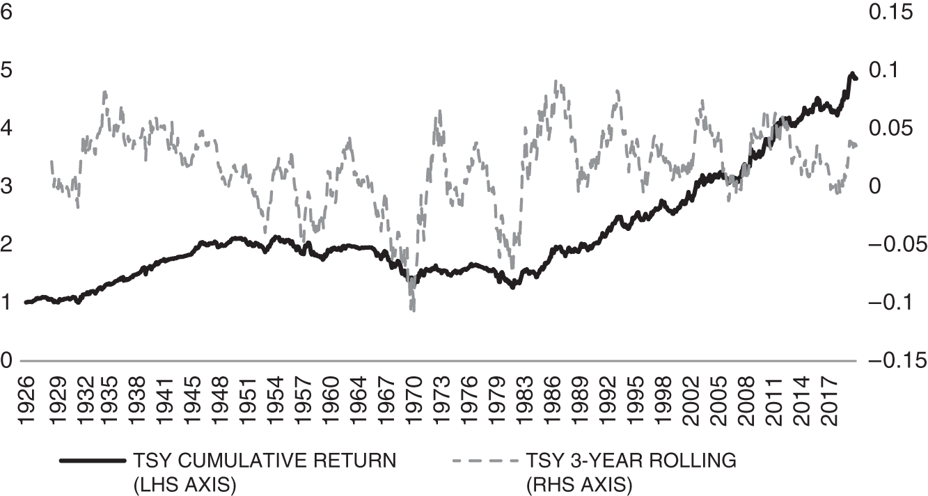
EXHIBIT 2.8 Cumulative and rolling 36‐month excess returns for US government bonds.
Source: Ibbotson's US Long‐Term Government Bond Total Return minus Ibbotson's US Treasury Bill Total Return from 1926 to 1972 and Bloomberg US Treasury index since 1973.
Although there have been very attractive risk‐adjusted returns for holding long‐term government bonds over the past century, there have been extended periods of underperformance. Long‐term government bonds have experienced a couple of lean decades in the middle of the past century, but experienced stellar returns over the last few decades with the secular decline in interest rates and yields. Combining Exhibit 2.8 with the declining and low yields seen in Chapter 1, it is natural to ask whether investing in government bonds (core fixed income) is still worthwhile.
All investors would agree that if your investment view were that yields will increase going forward, then tactically you would reduce allocations to core fixed income. However, simply noting that yields are low, and therefore yields must rise, is too naïve. Equation 2.14 notes that yields are expected to be low if current short‐term interest rates are low, expected future short‐term interest rates are low and the term premium is low. At the time of this writing (the end of 2021), yields are low because the determinants of yields suggest so. We will revisit tactical investment decisions for fixed income in Chapter 3. Our purpose here is to make the strategic case for investing in long‐term government bonds to harvest the term premium. There is a century of evidence to support this on a stand‐alone basis. In the next section we will see how fixed income diversifies alongside equity to provide a more balanced overall portfolio.
2.2.2 Credit Premium
The credit premium is the additional return an investor expects to receive from holding a risky bond relative to the return from holding a similar riskless bond. The risky and riskless bonds are similar in their cash flow profiles; they differ in terms of the probability of getting paid your coupons. A riskless government bond has zero probability of nonpayment, whereas for riskier corporate issuers there is a nonzero probability of nonpayment. The greater the risk of nonpayment, the greater the need for the expected return to compensate the investor.
It is possible to quantify the extent of this risk ex ante. In Chapter 1 we talked about a “spread” and this is a market‐implied view of the credit risk of the issuer. The spread can be computed by taking the difference in yields between the riskless and risky bonds with identical cash flows. If we extend our example of a 10‐year coupon‐bearing bond from Chapter 1, we can price that bond assuming the issuer is riskless, as in Equation (2.15), or risky, as in Equation (2.16):

The only difference across Equations 2.15 and 2.16 is the discount rate. For the riskless bond we use a risk‐free discount rate, ![]() , such as a government bond yield. For the risky bond we use a different discount rate,
, such as a government bond yield. For the risky bond we use a different discount rate, ![]() , such as a corporate bond yield. Generally speaking,
, such as a corporate bond yield. Generally speaking, ![]() , and the difference is the spread, that is,
, and the difference is the spread, that is, ![]() , and, because spreads are positive,
, and, because spreads are positive, ![]() , the price of the risky bond will be below that of the similar riskless bond,
, the price of the risky bond will be below that of the similar riskless bond, ![]() .
.
The credit spread is an ex‐ante measure of the return potential from exposure to credit risk, analogous to yield as an ex‐ante measure of the return potential from exposure to the term premium. We will have much to say on the determinants of credit risk, and hence credit spreads, later in Chapter 6 when we examine the default process in greater detail. Now, let's look at the data to see whether investors have been compensated for bearing credit risk.
Using an updated data series from Asvanunt and Richardson (2017) covering the 1926–2020 period, we can examine the long‐run evidence from investing in long‐term corporate bonds. There are a variety of corporate bonds to select from for this exercise. To ensure consistency with the data historically, we will focus on investment‐grade‐rated corporate bonds (the high‐yield market did not really develop until the 1980s). The source data for this time series is Ibbotson's US Long‐Term Corporate Bond Total Return for the 1926–1988 period and Bloomberg Indices (LUAC) for 1988–2020. Estimates of credit excess returns prior to 1988 require empirically estimating interest rate sensitivities. Asvanunt and Richardson (2017) describe the details, but the basic idea flows from an understanding of what duration is. If we have access to corporate bond returns (we do, Ibbotson data goes back to 1926), and we can observe contemporaneous changes in government bond yields (we do, bond yield data also goes back at least as far as 1926), you can then approximate duration. A simple regression of the total returns of corporate bonds onto changes in government bond yields will produce a regression coefficient. That regression coefficient tells you the change in corporate bond prices (i.e., returns) for a given change in yield. And that is duration! Asvanunt and Richardson (2017) applied this approach to a century of corporate bond data and found reliable evidence of a credit risk premium. Using updated data through to 2020, Exhibit 2.9 shows the cumulative and rolling three‐year average returns for US corporate bonds. Over the 1926–2020 period, the full sample Sharpe ratio is 0.48, again favorable to the 0.34 for the term premium and 0.44 for the equity risk premium over the same period. There is considerable variation in the performance of corporate bonds through time. It is also worth noting that this series only covers investment‐grade corporate bonds issued in the United States. There is a broader set of corporate issuers in many other countries, and for the last few decades there has been a large, and growing, set of high‐yield corporate bonds. The century of evidence in Exhibit 2.9 may understate the magnitude of the credit risk premium.
Some additional caveats are necessary for Exhibit 2.9. The quality of the data back in time is lower, and of particular concern is the completeness of the data with respect to default events. If defaults or other large negative return realizations are missing, this will lead to an overstatement of the credit premium. Although care has been taken to obtain the highest‐quality data possible, there are still limitations with older corporate bond return data. Indeed, Kizer, Grover, and Hendershot (2019) suggest that removing the first couple of decades reduces the size of the credit risk premium. Although in a strict sense that is correct, the pervasiveness of the credit‐risk premium across geographies, rating categories, and its existence in both cash and index derivative markets makes its existence noncontroversial. A fun exercise for the reader is to use the century of data and find periods where there is no credit risk premium or select random periods and see how frequently you find a positive risk‐adjusted return (the same can be done for the equity risk premium and term premium). I find this helpful to remind students what a risk premium means: over a long period the average return is positive, but in any one period it is not guaranteed to be positive. This also starts to get students thinking about what causes temporal variation in risk premium, setting up tactical investment decisions that we will cover in Chapter 3.
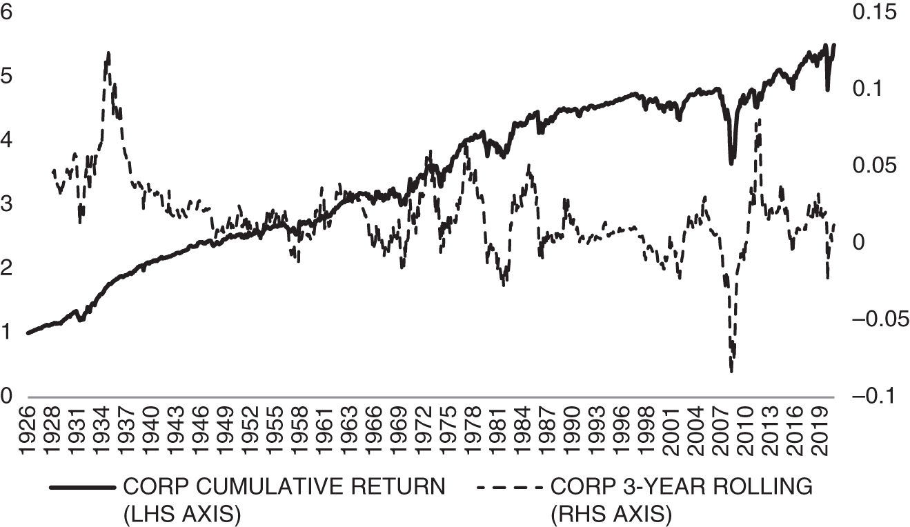
EXHIBIT 2.9 Cumulative and rolling 36‐month excess returns for US corporate bonds.
Source: Ibbotson's US Long‐Term Corporate Bond Total Return minus empirical‐duration‐matched long‐term government bonds from Ibbotson's US Long‐Term Government Bond Total Return. From 1926–1935, durations are estimated using in‐sample regressions. From 1936–1998, they are estimated using rolling 10‐year regressions. Full details in Asvanunt and Richardson (2017). Excess returns post 1988 are from Bloomberg Indices (LUAC).
2.2.3 Prepayment/Complexity/Volatility Premium
One other large set of fixed income securities is the “securitized” market. This includes a wide variety of bonds whose cash flows are linked to cash flows from other obligations. They are a repackaging of existing contractual commitments. There are sound economic reasons for these repackaged bonds: they allow for improved risk sharing among capital market participants. Of course, that efficient risk sharing only works if those market participants understand the risks that they are sharing in. Some would say that the Great Financial Crisis is the poster child for a lack of such understanding. In any event, the securitized market is here to stay. As we noted in Chapter 1, the Global Securitized subcategory accounted for approximately $9 trillion USD, out of the $68 trillion USD outstanding bonds in the Global Aggregate. The securitized market is very large. Within this category, however, there are many different types of securitized bonds.
The Bloomberg Global Securitized index includes securitized bonds from four broad categories: (i) agency mortgage‐backed passthrough securities, (ii) asset‐backed securities, (iii) commercial mortgage‐backed securities, and (iv) covered bonds. Agency MBS includes the passthrough bonds issued by government agencies including GNMA (Ginnie Mae, or the Government National Mortgage Association), FHLMC (Freddie Mac, or the Federal Home Loan Mortgage Corporation), and FNMA (Fannie Mae, the Federal National Mortgage Association). This category accounts for 75 percent of the total global securitized market (Bloomberg indices) as at December 31, 2020, and the majority of these are 30‐year conventional fixed rate mortgages. These three entities are all government sponsored, whose purpose is to provide backing and security to a vast array of home mortgage loans facilitating home ownership in the United States. The passthrough securities are pools of underlying mortgages backed by each respective entity. New bonds are issued backed by the cash flows of the pool and they are guaranteed by the respective agency that takes a fee for that guarantee and associated mortgage servicing activities. If these bonds are guaranteed, one may ask what is the risk that would require compensation? It is the risk of payment at different times than initially contracted. The underlying mortgage holders may refinance for a variety of reasons and hence pay early. This prepayment risk is a unique source of risk underlying mortgage‐backed securities.
Asset‐backed securities within the Bloomberg Global Securitized Index accounted for a little over $100 billion USD as of December 31, 2020, and they typically cover credit card, automobile, and business‐related loans. These bonds contain their own issuer‐specific credit risk and associated prepayment risks. Commercial mortgage‐backed securities (CMBSs) within the Bloomberg Global Securitized Index accounted for approximately $570 billion USD as of December 31, 2020. These CMBSs cover a wide range of securitized bonds including guaranteed bonds linked to multifamily residential properties, small businesses, and project loans. These bonds can be single‐tranche or multitranche facilities, which adds a further layer of complexity to the securitization. The covered‐bonds category within the Bloomberg Global Securitized Index accounted for around $1.4 trillion USD as at December 31, 2020, and is almost exclusively related to mortgage loans issued outside the United States (typically by European financial institutions).
What all the securitized bonds share is a risk associated with early prepayment. That risk commands a premium in the form of a spread over cash‐flow‐matched riskless government bonds. In some cases, there will also be credit risk associated with the underlying entity creating and servicing the securitized debt. Estimating the duration profile of these securitized bonds, so as to measure spreads, can be very challenging, as the future cash flows are dependent on current interest rates and expected paths of future interest rates. The behavior of the underlying mortgage holders may also need to be modeled in response to your forecasted future path of interest rates. This is no easy task, and different smart people trying to estimate the same interest rate sensitivities may end up with very different answers.
Diep, Eisfelt, and Richardson (2021) examined the prepayment risk premium embedded in the US securitized market using 30‐year fixed‐rate bonds backed by Fannie Mae. This involved assessing the return profile across the “coupon stack.” At a point in time there will be outstanding pooled mortgages from various points in time, so while new fixed‐rate mortgages all have a similar rate, over time, as interest rates change, there will be heterogeneity in the coupon rate across different mortgage pools. Some pools will have a coupon rate above (below) the prevailing market mortgage rate and they are called premium (discount) bonds. This variation in coupon rates across mortgage pools gives rise to prepayment risk. Mortgages that have a coupon rate higher than prevailing interest rates are at risk of having the underlying mortgages repaid earlier, leaving the holder of the MBS at risk of having to reinvest those proceeds at a lower rate. You thus expect to see spreads on mortgage‐backed securities to be larger when deviating further from “par”; that is, mortgage bonds with an underlying coupon rate higher than prevailing rates are at greater risk of prepayment, so they are worth less and hence carry a higher spread. Consistent with this, Diep, Eisfelt, and Richardson (2021) find an upward‐sloping pattern of spreads and coupon rates (i.e., spreads are higher for premium MBS), but that pattern is concentrated when there are more premium coupon bonds outstanding (and the risk bearing capacity of capital‐constrained participants in securitized markets is lower, so capital‐constrained market participants therefore command a greater premium). In markets in which there are more mortgage pools with coupon rates below prevailing market rates (i.e., the supply of MBS is dominated by discount MBS) the opposite is true: discount coupons attract higher spreads. The market price of prepayment risk is time varying.
Why all this seemingly technical discussion? This will be clear when we look at the return profile of excess returns for securitized bonds. Exhibit 2.10 shows the cumulative and rolling three‐year average returns for US MBS. Over the 1988–2020 period the full sample Sharpe ratio is 0.26, which is only slightly smaller than the risk premia observed for the term premium and credit premium. This Sharpe ratio of 0.26 is considerably lower than the 1.34 reported in Exhibit 2.1 because we are now talking about the nonrate component of returns (i.e., excess returns over duration marched government bonds, not excess returns over cash). Over this time period, the rate component of returns for all fixed income assets was strongly positive. Still, a Sharpe ratio of 0.26 is economically meaningful, but it does mask an exceptionally low average excess return (about three basis points annualized over this period). What is causing this? It could be measurement error in the estimates of duration used to measure spreads. This is likely not the culprit, as similar patterns of tiny excess returns are observed using estimates of duration across different index providers or using empirical estimates of duration. The source of the small average excess return is that the MBS index has most of its securities outstanding at close to par (prevailing mortgage rates). This means that most securitized bonds included in the index are not sensitive to prepayment shocks ($100 notional will return $100). They will be sensitive to volatility in interest rates because there may be future prepayment risk for these bonds, but that effect is small. Attempts to capture the prepayment risk premium need to focus on securities that are distant from par (i.e., premium and discount securities in the “wings” of the coupon stack) and ideally condition exposure to discount and premium bonds based on the prevailing market price of prepayment risk. The greatest excess return potential for securitized assets resides in the less liquid corners of this market (e.g., nonagency securitized bonds and far out of the money mortgage pools).
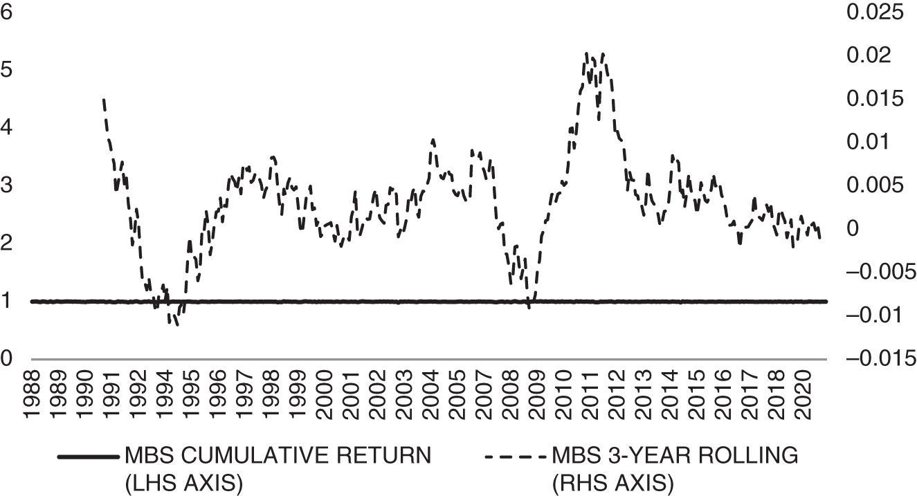
EXHIBIT 2.10 Cumulative and rolling 36‐month excess returns for US mortgage‐backed securities.
Source: Data from Bloomberg Indices (LUMS). Data is for the period 1988–2020.
We could add further categories of fixed income risk premia. The two most obvious categories would be for emerging and private markets. An emerging market fixed income risk premium would reflect the combination of return opportunities across emerging market local currency bonds, emerging market hard currency bonds, and emerging currency returns. The emerging market corporate risk is very similar in spirit to the developed market credit premia already discussed, and the emerging market local currency (mostly government bonds) is like the developed market term premium already discussed. Extending the cross‐section of government and corporate bond issuers beyond developed markets will provide additional diversification benefits as the risks underlying term premium (inflation and growth shocks) and credit premium (growth shocks) can be diversified internationally. Finally, emerging market hard currency bonds share some similarity to the general credit risk premium, and we will discuss this market in detail in Chapter 7.
Private credit markets are a growing segment of the fixed income market. Interest from asset owners has ballooned over the last five years. Although data for this market is hard to identify, there are some index providers. A commonly used benchmark is the Cliffwater Direct Lending Index. It seeks to measure the unlevered, gross of fee performance of US middle‐market corporate loans, as represented by the asset‐weighted performance of the underlying assets of Business Development Companies (a BDC is an organization that invests in small‐ and medium‐sized companies as well as distressed companies). This total return index includes income return, and realized and unrealized gains and losses. As with all private markets, there is concern about the quality of marks giving rise to unrealized gains and losses. That said, the annualized return for private markets over the 2004–2020 period is 9.1 percent with an associated Sharpe ratio of 2.47. This is amazing. Part of this return may be attributable to operating and investing efficiency from direct lending activities and excellent security selection. But part of this is attributable to the smoothing benefit of private markets (i.e., the stale data issue mentioned in Chapter 1). To corroborate this assertion, the annualized total return of the Bloomberg High Yield Index (LF98) over the 2004–2020 period was 7.6 percent and an associated Sharpe ratio of 0.83. This is a lot smaller than the 2.47 Sharpe ratio for private markets over the same period, but the difference is primarily attributable to return volatility, not to the level of returns. Private markets are another way to capture the credit risk premium, but it is not clear how diversifying they really are. And for some direct‐lending activities that have short track records, there is concern about security selection around default risk. Private credit markets have the potential to add to credit risk premium, but more data analysis is needed.
2.3 THE STRATEGIC DIVERSIFICATION BENEFIT OF FIXED INCOME
We can now put what we have learned together to think about broader asset allocation decisions. Why do we allocate to fixed income markets, and subcategories within fixed income markets? Section 2.2 illustrated stand‐alone evidence supporting (i) investments into government bonds to harvest the term premium, (ii) investments into corporate bonds (and other credit‐sensitive assets) to harvest the credit premium, and (iii) investments into securitized markets to harvest the prepayment premium. But are these risk premia additive in the context of the asset owner's overall portfolio? This is particularly important in the context of investments into the less liquid, and hence more costly to trade, corners of the fixed income markets like corporate and securitized bonds. Don't incur transaction costs and introduce liquidity risk to your portfolio unless you are compensated for doing so.
Let's start with the empirical fact that equity markets (public and private) are represented in most, if not all, asset owner portfolios. The equity risk premium has long been the base building block of asset allocation. Government bonds are added to equities in the classic 60/40 portfolio (60 percent capital allocated to equities and 40 percent allocated to bonds). The ubiquitous nature of the 60/40 portfolio reflects the fundamental strategic diversification benefit of fixed income relative to equities. Indeed, there are now many risk parity variants (e.g., Bridgewater, PanAgora, AQR etc.) that prudently utilize leverage to allocate across stocks and bonds (and other diversifying asset classes) to balance the risk contribution across different types of risk premia and still deliver equity‐like returns. Our focus here will be simpler and just noting how and why it is that fixed income diversifies equity.
Exhibit 2.11 shows the annualized return of US government bonds and US stocks over the 1926–2020 period using rolling 10‐year periods to estimate annualized returns. The exhibit also shows the correlation between US bonds and US stocks over the past 120 months. The correlation between stocks and bonds has varied enormously over this period, but it has only been reliably negative for the past couple of decades. A 60/40 combination of US bonds and US stocks generates a full sample Sharpe ratio of 0.49 that exceeds the 0.44 (0.35) Sharpe ratio for US stocks (bonds) over the same period. This higher risk‐adjusted return is due to the less than one correlation between stocks and bonds and the fact that they both have a similar return per unit of risk. Of course, the unlevered 60/40 portfolio generates a total return that is lower than that of equities (5.6 percent annualized return for 60/40 vs. 8.2 percent annualized returns for US stocks), but leverage can increase the return of the 60.40 portfolio to 9.1 percent and yield the same overall volatility of the US stocks only portfolio.

EXHIBIT 2.11 Annualized returns and rolling 10‐year correlation for US bonds and US stocks.
Sources: Combination of Ibbotson's Long‐Term Government Bond Total Return, Barclays US Treasury total returns, and Standard & Poor's Indices. Data is for the period 1926–2020.
US bonds help diversify a US stock‐only portfolio. Similar results can be found looking at global bond and global stock portfolios. Why is this the case? Stocks as the residual claim against free cash flows generated by corporations are exposed to underlying macroeconomic variables: growth and inflation. Stocks have a positive exposure to economic growth shocks (stock prices rise and fall with changing expectations of the business cycle). Stocks have a relation to inflation shocks (generally they fare better in lower inflationary environments, but this relation is more subtle – see e.g., Ilmanen, Maloney, and Ross 2014). Government bonds, as we discussed in Section 2.2, are also exposed to growth and inflation. Improving business cycle outlook or increasing inflation leads to more cautionary monetary policy and higher yields (hence lower returns), whereas worsening business cycle outlook or falling inflation leads to more accommodative monetary policy and lower yields (hence higher returns). It should therefore be clear that stocks and bonds structurally have a different sign on their sensitivity to growth shocks (growth shocks are good for stocks and bad for bonds), but a similar sign on their sensitivity to inflation shocks (inflation shocks are bad for stocks but even worse for bonds). It is this difference in sensitivities to underlying macroeconomic state variables that creates the diversification benefit across stocks and bonds. Of course, there are other drivers of stock and bond returns including (i) aggregate risk aversion that would increase the common component of stock and bond returns, and (ii) sentiment or net demand factors from capital market participants seeking safe‐haven assets that decrease the common component of stock and bond returns. Indeed, the temporal variation in the strength of the correlation between stocks and bonds in Exhibit 2.11 shows how these economic forces are varying through time and affecting stocks and bonds differently throughout time.
Another way to see the diversification benefit of stocks and bonds is to examine similarities in their downside risk based on drawdown profiles (i.e., peak to trough decline). Exhibit 2.12 computes the drawdown profile of US stocks and US bonds over the 1926–2020 period. The return series are converted to a price index, and each month is then identified as having a price that is below (or at or above) the prior maximum price level. If the current price index is below a prior maximum, then a drawdown is identified. Exhibit 2.12 shows the cumulative return profile of drawdown periods over the last century. US stocks have larger drawdowns (stock returns are more volatile). The fact that the drawdowns (either in length or severity) do not perfectly align is evidence of diversification in the left‐tail of return realizations.
Statistically, we can do even better. Utilizing the data for the past century, we can simultaneously solve for the optimal set of portfolio weights across government bonds, corporate bonds, and stocks that would have yielded the highest Sharpe ratio. This procedure is described in detail in Asvanunt and Richardson (2017), and I note the relevant material here. We need to solve for the ex‐post optimal allocation weights for a portfolio consisting of corporate bonds, government bonds, and stocks subject to no shorting and leverage constraints, namely

EXHIBIT 2.12 Drawdowns for US bonds and US stocks over the 1926–2020 period.
Sources: Ibbotson's US Long‐Term Government Bond Total Return minus Ibbotson's US Treasury Bill Total Return from 1926 to 1972 and Bloomberg US Treasury index since 1973. Standard & Poor's data for US stocks.
R is a vector of average corporate bond, government bond, and stock excess returns; w is the vector of portfolio weights to be solved for; and ![]() is the corresponding excess return covariance matrix. The optimal portfolio solution is mean‐variant efficient. An important caveat for the large asset owner is that this analysis does not incorporate information on the expected transaction costs or capacity of each asset, and as such the results here should be interpreted with caution for large asset allocation decisions. Capacity considerations would reduce the importance of less liquid assets (e.g., corporate bonds and/or credit index derivatives) in the overall portfolio.
is the corresponding excess return covariance matrix. The optimal portfolio solution is mean‐variant efficient. An important caveat for the large asset owner is that this analysis does not incorporate information on the expected transaction costs or capacity of each asset, and as such the results here should be interpreted with caution for large asset allocation decisions. Capacity considerations would reduce the importance of less liquid assets (e.g., corporate bonds and/or credit index derivatives) in the overall portfolio.
For the 1926–2020 period, the optimal weights are 55 percent for corporate bonds, 36 percent for government bonds, and 9 percent for stocks. Of course, this analysis can be run for different time periods with very different optimal weights. For the period 1973–2020 (which is the period after the original Lehman indices that pre‐date the Bloomberg Indices started) the optimal weights are 23 percent for corporate bonds, 63 percent for government bonds, and 14 percent for stocks.
A potential limitation of this optimal weight analysis is that it is based on a mean‐variant analysis of returns, which may be less relevant when the underlying distribution of returns is not normal. Asvanunt and Richardson (2017) assess whether the inference that the credit risk premium is additive to both the term and equity risk premium is robust to return nonnormality. That analysis uses the Sortino ratio (e.g., Sortino and Price 1994):
where T is the target or required rate of return (for simplicity, we set the target return to 0 percent), and

Given our choice of a 0% target return, the numerator of our Sortino ratio will be the same as that for the Sharpe ratio. The difference is in the denominator, where the Sortino ratio only “penalizes” return realizations that are below the target return. Both the frequency and magnitude of below‐target returns are penalized. For the period 1926–2020 the optimal weights that maximize the Sortino ratio are as follows: 51 percent for corporate bonds, 39 percent for government bonds, and 10 percent for stocks. There is consistent evidence that fixed income allocations are important for overall portfolio diversification.
2.4 IS THE STRATEGIC DIVERSIFICATION BENEFIT OF FIXED INCOME THREATENED IN A LOW‐INTEREST‐RATE ENVIRONMENT?
We have seen that fixed income as an asset class diversifies equity risk for asset‐owner portfolios. And we have an understanding about why that diversification exists. Yet, the last decade has seen many question the role of fixed income in their overall portfolio. This skepticism is typically anchored in a strong belief in mean reversion. If government bond yields are low, they must revert to a higher level. And if the fear is that mean reversion will happen soon, that fear leads to an investment decision: reduce allocations to the asset class with near‐term expected losses. Although rising yields do not automatically lead to negative returns, because carry still has a positive expected return (i.e., the change in the yield multiplied by duration needs to exceed the initial yield), directionally rising yields mean lower future returns.
Is that fear of rising yields rational? The discussion of term premium in Section 2.2 tells us that long‐term government bond yields are determined by current short‐term interest rates, expected short‐term interest rates in the future, and the term premium (a catch‐all for risk aversion, sentiment, and general macroeconomic uncertainty). The low yields today might be justified if we look at the economic backdrop (low levels of inflation, low levels of economic growth, and central banks universally consistent in their use of monetary policy to help stimulate the real economy). Although inflation and growth expectations remain low, government bond yields may remain low for the foreseeable future. What does this mean for fixed income investors? There is still the potential for positive returns by allocating to long‐term government bonds. And this is especially true for the investor who can make use of derivatives to maintain a constant‐maturity exposure to a long‐dated government bond (e.g., 10‐year Treasury Note Future). Although the shape of the yield curve remains upward sloping, the positive yield at the 10‐year point (at least true in the United States) combined with attractive roll‐down properties makes for attractive positive returns from exposure to the term premium. Investors do, however, need to keep in mind that yields are much lower today than they have been over the last century. This means lower levels of returns and, for the investor who is unable to utilize leverage, fixed income is less attractive today than it has been historically. For the investor who can utilize leverage, fixed income may still be as attractive as it ever was. It does not mean fixed income allocations should go to zero! Just because fixed income markets may look relatively expensive compared to history (that's what a low yield means), it is not the case that other asset classes, such as stocks, are any less expensive. Fixed income still preserves its diversification benefit.
REFERENCES
- Asvanunt, A., and S. Richardson. (2017). The credit risk premium. Journal of Fixed Income, 26, 6–24.
- Brooks, J. (2021). What drives bond yields. AQR working paper.
- Diep, P., A. Eisfelt, and S. Richardson. (2021). The cross‐section of MBS returns. Journal of Finance, 76, 2093–2151.
- Gilchrist, S., B. Wei, V. Yue, and E. Zakrajsek. (2021). The Fed takes on corporate credit risk: An analysis of the efficacy of the SMCCF. NBER working paper.
- Holston, K., T. Laubach, and J. Williams. (2017). Measuring the natural rate of interest: International trends and determinants. Journal of International Economics, 108, S39–S75.
- Ilmanen, I., T. Maloney, and A. Ross. (2014). Exploring macroeconomic sensitivities: How investments respond to different economic environments. Journal of Portfolio Management, 40, 87–99.
- Kizer, J., S. Grover, and C. Hendershot. (2019). Re‐examining the credit premium. Buckingham Strategic Wealth, working paper.
- Laubach, T., and J. Williams. (2003). Measuring the natural rate of interest. Review of Economics and Statistics, 85, 1063–1070.
- Sortino, F. A. and L. N. Price (1994). Performance measurement in a downside risk framework. Journal of Investing, 3, 59–64.