
CHAPTER 6
Security Selection – Credit‐Sensitive Assets
OVERVIEW
This chapter lays out the investment opportunity set for credit‐sensitive assets. Our focus is on developed market corporate bonds, but the insights we cover can be extended to emerging market government bonds. We look at the vast number of investment grade (IG) and high yield (HY) corporate bonds in developed market indices and note the first order importance of across issuer security selection. While security selection among corporate bonds shares some similarities with security selection among stocks, we note important differences between credit and equity investing. The chapter discusses the intuition behind representative measures of value, momentum, carry, and defensive investment themes and evaluates the success of these strategies individually and in combination for developed corporate bond markets.
6.1 WHAT IS THE INVESTMENT OPPORTUNITY SET FOR DEVELOPED MARKET CORPORATE BONDS?
We will use a representative broad corporate bond index to explore the potential investment opportunity set. We will use indices from ICE/BAML for this purpose. To get a sense of the current size of the corporate bond markets, how those markets have grown over the past 20 years, and what the typical corporate issuer looks like, we examine four distinct categories of corporate bonds: (i) US IG includes all CAD‐ and USD‐denominated bonds issued by corporate issuers domiciled in developed markets within the ICE/BAML G0BC index, (ii) US HY bonds (ICE/BAML H0A0 index), (iii) European (EU) IG includes all GBP‐ and EUR‐denominated bonds issued by corporate issuers domiciled in developed markets within the ICE/BAML G0BC index, and (iv) EU HY bonds (ICE/BAML HP00 index). All bonds are issued by corporations domiciled in developed markets. There is nothing limiting the efficacy of systematic investing approaches for emerging market corporate bonds, but the challenges of data access and liquidity in emerging markets can make that effort more challenging. We will not be looking at emerging corporate bonds in this chapter.
What types of bonds are included in these indices? The G0BC index, from which we construct our two IG universes, contained nearly 17,000 bonds as of December 31, 2020. And our US (EU) IG subuniverses contained 8,802 (3,443) corporate bonds, respectively. The G0BC index is designed to track the performance of investment grade corporate debt publicly issued in the major domestic and Eurobond markets. All securities are IG rated based on an average rating across the main rating agencies, have a minimum of 12 months remaining to final maturity, a fixed coupon schedule, and meet minimum issue size requirements (e.g., $250 million USD for a USD denominated bond). The H0A0 (HP00) index used for our US (EU) HY universes contained 2,030 (808) bonds, respectively, as of December 31, 2020. The H0A0 index is designed to track the performance of USD denominated subinvestment grade corporate debt publicly issued in the US domestic market. The HP00 index is designed to track the performance of EUR and GBP denominated sub investment grade corporate debt publicly issued in the eurobond, sterling domestic, or euro‐domestic markets. Both H0A0 and HP00 follow similar index inclusion rules to G0BC (i.e., all securities are HY rated based on an average rating across the main rating agencies, have a minimum of 12 months remaining to final maturity, a fixed coupon schedule, and meet minimum issue size requirements). H0A0 has the additional requirement that eligible securities must have risk exposure to FX‐G10 countries (Euro members, US, Japan, UK, Canada, Australia, New Zealand, Switzerland, Norway, and Sweden), so emerging corporate issuers are explicitly excluded. All four corporate bond universes are market capitalization weighted (see the discussion at the end of Chapter 5 for arguments for and against this weighting choice).
Exhibit 6.1 shows the market capitalization in USD trillions for the four corporate bond universes. There has been a huge growth in these markets. As of December 2020, the total market capitalization of corporate bonds across our four universes is $14.05 trillion dollars, led by US IG ($8.12T) and European IG ($3.84T). The HY markets are smaller with $1.55T ($0.54T) outstanding for US (European) markets, respectively.
What is the composition of corporate issuers across our corporate bond universes? As with government bonds, there are multiple corporate bonds outstanding for a given corporate issuer. The concentration of issues per issuer is not as great as was seen in the government bond market. Exhibit 6.2 plots the number of unique issuers across the four indices. There has been substantial growth in the number of corporate issuers over the 1996–2020 period. So part of the growth in the overall corporate bond market is attributable to a growing number of companies seeking to raise debt financing in public bond markets. As of December 31, 2020, there were 1,206 (602) issuers in the US (EU) IG markets, and 860 (384) issuers in the US (EU) HY markets.
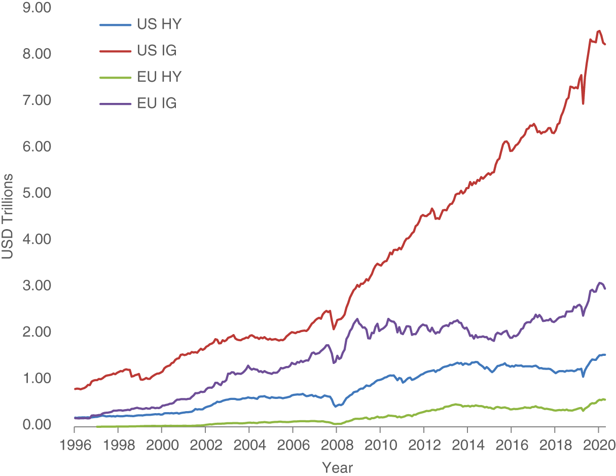
EXHIBIT 6.1 Market capitalization (USD) of developed‐market corporate bond indices. US IG includes all CAD and USD denominated bonds issued by corporate issuers domiciled in developed markets within the ICE/BAML G0BC index. US HY is the US High Yield Index from ICE/BAML (ticker H0A0). EU IG includes all EUR and GBP denominated bonds issued by corporate issuers domiciled in developed markets within the ICE/BAML G0BC index. EU HY is the European Currency High Yield Index from ICE/BAML (ticker HP00).
Source: ICE/BAML indices.
Exhibit 6.3 plots the number of issues across the four indices. There is a clear increase in the number of issues (bonds) over time reflecting the general increase in the size of corporate bond markets. The occasional “‘drops”’ in number of issues are attributable to changes in index inclusion rules (e.g., changes in the minimum allowable size of the bond). As of December 31, 2020, there were 8,802 (3,443) issues in the US (EU) IG markets, and 2,030 (808) issues in the US (EU) HY markets. Exhibits 6.2 and 6.3 imply that the average issuer in the US (EU) IG market currently has about seven (six) bonds outstanding, and the average issuer in the US (EU) HY market currently has about two (two) bonds outstanding. This creates potential for both across and within issuer security selection, but note that the breadth of within issuer investment choices is much smaller relative to government bonds, especially for HY corporate bonds.
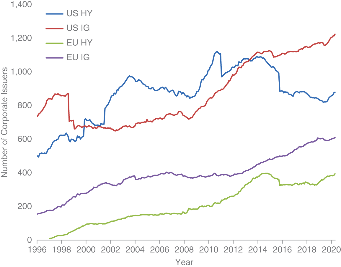
EXHIBIT 6.2 Number of corporate issuers across developed market corporate bond indices. US IG includes all CAD and USD denominated bonds issued by corporate issuers domiciled in developed markets within the ICE/BAML G0BC index. US HY is the US High Yield Index from ICE/BAML (ticker H0A0). EU IG includes all EUR and GBP denominated bonds issued by corporate issuers domiciled in developed markets within the ICE/BAML G0BC index. EU HY is the European Currency High Yield Index from ICE/BAML (ticker HP00).
Source: ICE/BAML indices.
What does the duration of corporate bonds look like? The duration profile of corporate bonds is considerably shorter than government bonds. Exhibit 1.12 in Chapter 1 showed that the duration of the global treasury component of the Global Aggregate Index was about nine years as of December 31, 2020. Exhibit 6.4 shows the duration profile of our four corporate bond universes.
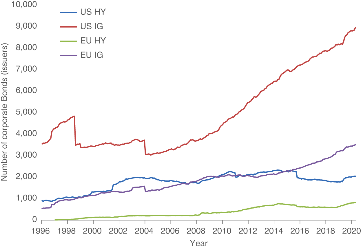
EXHIBIT 6.3 Number of corporate bonds (issues) across developed‐market corporate bond indices. US IG includes all CAD and USD denominated bonds issued by corporate issuers domiciled in developed markets within the ICE/BAML G0BC index. US HY is the US High Yield Index from ICE/BAML (ticker H0A0). EU IG includes all EUR and GBP denominated bonds issued by corporate issuers domiciled in developed markets within the ICE/BAML G0BC index. EU HY is the European Currency High Yield Index from ICE/BAML (ticker HP00).
Source: ICE/BAML indices.
The average duration for the US (EU) IG universe is 8.21 (5.82) years as of December 31, 2020, and for the US (EU) HY universe it is 3.55 (3.32) years, respectively. Corporate bonds tend to have a lower duration than government bonds, and there is a striking difference between IG and HY bonds. This difference is a direct consequence of the heightened credit risk of HY rated corporate issuers. Lenders rationally lend to riskier issuers for shorter periods of time. There is also a much greater skew to the duration distribution for US IG corporate bonds. This is a direct consequence of the long‐duration corporate bond market in the United States. Many corporate and public pension plans demand longer dated “‘safe”’ fixed income assets to help with asset‐liability matching needs, and US‐based corporates can tap into that demand by issuing longer dated bonds. We will discuss systematic approaches to long duration corporate bond indices in Chapter 11.

EXHIBIT 6.4 Duration of corporate bonds (issues) across developed‐market corporate bond indices. The bold black line is the average duration, the other three lines labeled 25, 50, and 75 represent percentiles. The vertical axis is effective duration measured in years.
Source: ICE/BAML indices.

EXHIBIT 6.5 Option adjusted spreads (OAS) of corporate bonds (issues) across developed‐ market corporate bond indices. The bold black line is the median OAS (labeled as 50). The other two lines labeled 25 and 75 represent percentiles (25 for lower quartile, and 75 for upper quartile). The vertical axis is credit spread measured in basis points (i.e., 300 means 3 percent).
Source: ICE/BAML indices.
What do credit spreads look like across our corporate bond universes? Exhibit 6.5 shows the cross‐sectional distribution of option adjusted spreads. An option‐adjusted spread is the credit spread adjusted for embedded optionality (e.g., calls) that reduces the duration profile of the corporate bond, which in turn affects the computed spread (i.e., you are matching the option‐adjusted cash flows to riskless government bond securities, not the full set of cash flows). It is clear across all corporate bond universes that there is a strong countercyclical pattern with credit spreads and the business cycle. Credit spreads widen considerably, and quickly, during periods of economic stress (e.g., the end of the dot.com boom in 2000–2001, the great financial crisis of 2008, and the COVID crisis in early 2020). The scales of the IG and HY charts are very different: high–yield‐rated corporate issuers are riskier and that is reflected in the considerably high credit spreads on average across the IG and HY markets.
There are interesting dynamics in credit spreads across IG and HY corporate bond markets. For most corporate issuers the credit spread term structure is upward sloping, especially for IG‐rated corporate issuers. The slope of the credit curve (i.e., the pattern in credit spreads as a function of maturity or duration) is typically flatter the riskier the corporate issuer (see, e.g., Arora, Richardson, and Tuna 2014). One well‐known feature of fixed income markets is that the return per unit of risk tends to be higher toward the front of the curve (see, e.g., Ilmanen 2011). We will capture that as part of our investment framework within the defensive theme. Leveraging the front end of credit (or yield) curves, via a passive steepener, has historically generated attractive risk‐adjusted returns. It is a return opportunity that is not without risk, as there can be large drawdowns from curves flattening, especially in times of crisis. For corporate bond investors this was a very sore point in March 2020 (during the start of the COVID crisis).
There is at least one other aspect of the corporate bond market that is important to highlight up front. Newcomers to the corporate bond markets need to appreciate that many corporate issuers do not have publicly listed equity. This can pose challenges sourcing relevant data for your investment process. It does not mean you cannot, or should not, invest into these “private” issuers, but it does mean you need to be careful in sourcing your data. Exhibit 6.6 shows the fraction of corporate issuers across our four corporate bond universes that do not have publicly listed equity. A sizable portion of corporate issuers are private, particularly in Europe. This will reduce the investment opportunity set for security selection when equity market data or data that comes with equity listings (e.g., quarterly financial statements and analyst coverage) is unavailable.
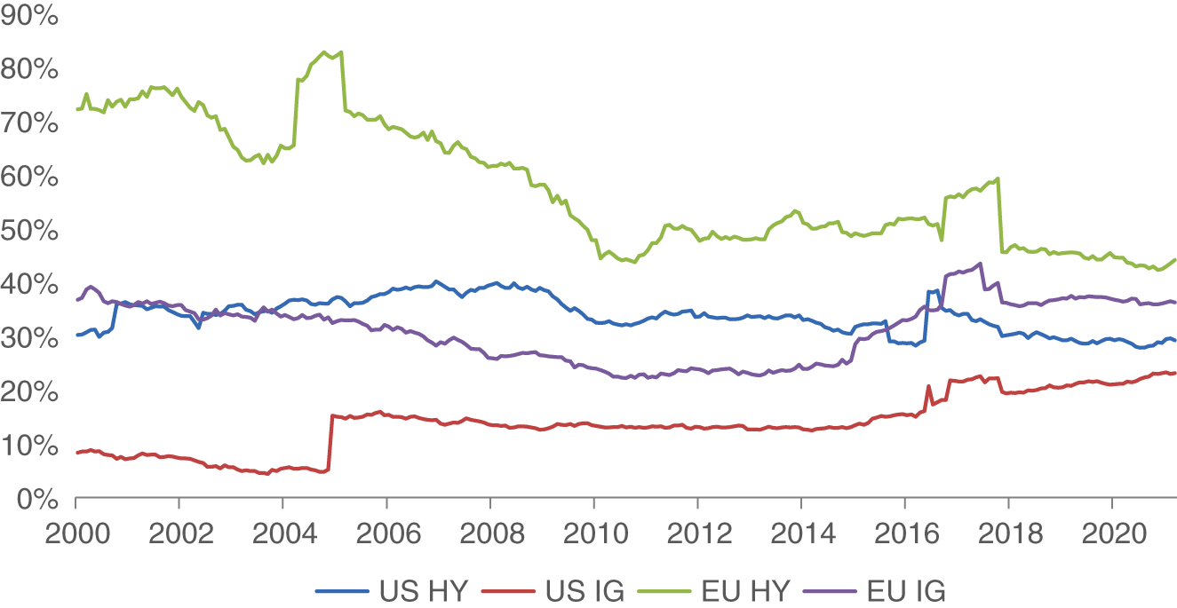
EXHIBIT 6.6 Fraction of private issuers across developed market corporate bond indices.
Source: ICE/BAML indices.
6.2 DIMENSIONS OF ACTIVE RISK TAKING WITHIN CORPORATE BONDS
6.2.1 Importance of Across Issuer Relative to Within Issuer
The cross‐section of corporate bonds is much larger than government bonds. US (EU) IG indices contain over 1,200 (600) issuers compared to the 13 sovereign entities in the JP Morgan Government Bond Index (GBI). Security selection for corporate bonds will, therefore, naturally focus on the across‐issuer dimension. The principal component analysis undertaken in Chapter 5 we will not repeat here for corporate bonds. But, to emphasize the importance of “level” effects and justify our focus on across issuer security selection, we will decompose credit‐spread changes at the issuer level into a common‐issuer component and a maturity‐specific component.
We can start with an approximation for credit excess returns (![]() ):
):
where ![]() is credit spread and
is credit spread and ![]() is spread duration. For each issuer that has multiple bonds outstanding, we can measure (i) the average spread change across all outstanding bonds,
is spread duration. For each issuer that has multiple bonds outstanding, we can measure (i) the average spread change across all outstanding bonds, ![]() , akin to the “level” approach taken for government bonds, and (ii) the relation between spread change and bond spread duration,
, akin to the “level” approach taken for government bonds, and (ii) the relation between spread change and bond spread duration, ![]() , akin to the “slope” approach taken for government bonds. This allows for an additive decomposition of spread change:
, akin to the “slope” approach taken for government bonds. This allows for an additive decomposition of spread change: ![]() (the residual here is necessary as we will estimate this decomposition empirically).
(the residual here is necessary as we will estimate this decomposition empirically). ![]() reflects the average widening or tightening of credit spreads across all bonds and represents a parallel shift in the credit curve.
reflects the average widening or tightening of credit spreads across all bonds and represents a parallel shift in the credit curve. ![]() captures how longer‐term bonds widened (or tightened) relative to shorter‐term bonds and represents a widening or flattening of the credit curve. The portion of credit‐excess returns attributable to spread changes can be written as
captures how longer‐term bonds widened (or tightened) relative to shorter‐term bonds and represents a widening or flattening of the credit curve. The portion of credit‐excess returns attributable to spread changes can be written as ![]() , where
, where ![]() is the spread duration for a specific bond for an issuer and
is the spread duration for a specific bond for an issuer and ![]() is the average spread duration across bonds of the issuer. This may be easier to grasp visually (see Exhibit 6.7).
is the average spread duration across bonds of the issuer. This may be easier to grasp visually (see Exhibit 6.7).

EXHIBIT 6.7 Breakdown of credit spread changes into level and slope components.
The dots in Exhibit 6.7 correspond to specific bonds for a corporate issuer. The vertical axis measures the change in spreads over a month, and the horizontal axis is the spread duration of each bond. The slope of the estimated regression line is ![]() , and
, and ![]() is the average across all bonds (indicated by the dashed horizontal line in Exhibit 6.7). The portion of
is the average across all bonds (indicated by the dashed horizontal line in Exhibit 6.7). The portion of ![]() attributable to the level and slope components need to be multiplied by spread duration. In the case of the slope component, the contribution to credit excess returns utilizes simple geometry: the “rise” is equal to the product of the “slope” (ΔSSLOPE, estimated via regression) and the “run”
attributable to the level and slope components need to be multiplied by spread duration. In the case of the slope component, the contribution to credit excess returns utilizes simple geometry: the “rise” is equal to the product of the “slope” (ΔSSLOPE, estimated via regression) and the “run” ![]() .
.
We can estimate this regression for all IG and HY issuers that have multiple bonds outstanding. This allows us to quantify the fraction of variation in ![]() that we can explain with either
that we can explain with either ![]() or
or ![]() and
and ![]() in combination. Estimating this using the full‐time series of returns for each corporate issuer, the level‐only specification can explain on average 60 (77) percent of variation in credit‐excess returns for IG (HY) corporates. Using both level and slope increases the return variation explained to an average 75 (90) percent for IG (HY), respectively. If you had a crystal ball, you would want to know the average credit spread change for the corporate issuer because this explains most of the credit‐excess returns. Thus, the level of credit spread changes, across issuer, will be the primary focus in the rest of the chapter.
in combination. Estimating this using the full‐time series of returns for each corporate issuer, the level‐only specification can explain on average 60 (77) percent of variation in credit‐excess returns for IG (HY) corporates. Using both level and slope increases the return variation explained to an average 75 (90) percent for IG (HY), respectively. If you had a crystal ball, you would want to know the average credit spread change for the corporate issuer because this explains most of the credit‐excess returns. Thus, the level of credit spread changes, across issuer, will be the primary focus in the rest of the chapter.
6.2.2 Investing in Credit Markets Is Not the Same as Investing in Equity Markets
A gentle reminder of the interdependence, but not equivalence, of claims across the capital structure is warranted. Even academics sometimes fail to remember this (I have seen multiple papers get submitted to academic journals where the analysis is simply a cut/paste from equity markets to credit markets). Expecting the same result in credit markets as you would expect for equity markets may be appropriate in some settings, but not always.
An equity investor participates in the free cash flow after all other claims have been paid; equity is the residual claim. There is no limit to the upside participation. An investor in a senior claim, such as a corporate bond or loan, participates in the free cash flow before the equity holder but only up to the point specified by the contractual terms of the fixed income security; the upside is strictly limited. Equity investing is very much about expectations of earnings and earnings growth (see, e.g., Penman 2001, and Penman, Reggiani, Richardson, and Tuna 2018). Equation (6.2) is a useful tautology based on a combination of the dividend discount model and clean surplus accounting:

![]() is the expected return for the equity claim,
is the expected return for the equity claim, ![]() is the expected (comprehensive) income for the next period, and
is the expected (comprehensive) income for the next period, and ![]() is the expected change in the premium of price over book value of equity. This latter term is what makes Equation (6.2) true (tautological), but it also captures the spirit of what equity investing is about: the long‐run future. You can think of the premium of price over book value as capturing expected earnings growth. Equity price integrates across all future periods for free cash flow (residual income) participation. So expected equity returns have an initial expected return component,
is the expected change in the premium of price over book value of equity. This latter term is what makes Equation (6.2) true (tautological), but it also captures the spirit of what equity investing is about: the long‐run future. You can think of the premium of price over book value as capturing expected earnings growth. Equity price integrates across all future periods for free cash flow (residual income) participation. So expected equity returns have an initial expected return component, ![]() , and additional expected returns that come from (risky) future earnings growth.
, and additional expected returns that come from (risky) future earnings growth.
In contrast, the expected returns for the corporate credit claim as shown in Equation (3.8) was linked to credit spreads and how they are expected to change. What determines credit spreads? The primary determinant of credit spreads is the expected loss given default (LGD) (see, e.g., Kealhofer 2003, and Correia, Richardson, and Tuna 2012). Technically, this is all in what is called “risk‐neutral” terms. That's just a fancy of way saying that there is a risk premium embedded in risky corporate bonds and the spreads that we infer from prices include that risk premium. Equation (6.3) captures this intuition:
![]() is the expected (risk neutral) default probability and
is the expected (risk neutral) default probability and ![]() is expected loss in the event of default (i.e.,
is expected loss in the event of default (i.e., ![]() is the recovery rate). Combining Equations (3.8) and (6.3) it should be clear that expected credit excess returns are driven by changing expectations of default and/or recovery rates. This is the downside focus of the credit investor who does not get to participate fully in future earnings growth. Credit investing is different from equity investing. In this chapter we will discuss how
is the recovery rate). Combining Equations (3.8) and (6.3) it should be clear that expected credit excess returns are driven by changing expectations of default and/or recovery rates. This is the downside focus of the credit investor who does not get to participate fully in future earnings growth. Credit investing is different from equity investing. In this chapter we will discuss how ![]() is a relevant fundamental input across our investment themes (e.g., value, momentum, and quality). We will not spend much time on recovery‐rate modeling because our focus is on security selection primarily across corporate issuers on a within sector basis. The key determinants of recovery rates are: (i) when you default (i.e., recovery rates are cyclical; lower in economic downturns), (ii) seniority (i.e., recovery rates are higher for loans than for secured bonds than for unsecured bonds), and (iii) sector/industry (i.e., recovery rates are linked to the nature of the assets that can be sold in the event of default to satisfy contractual commitments). As our security selection is in the cross‐section, within sector groups, and among corporate bonds that are similar in seniority (e.g., senior unsecured), recovery rates are of second‐order importance for us.
is a relevant fundamental input across our investment themes (e.g., value, momentum, and quality). We will not spend much time on recovery‐rate modeling because our focus is on security selection primarily across corporate issuers on a within sector basis. The key determinants of recovery rates are: (i) when you default (i.e., recovery rates are cyclical; lower in economic downturns), (ii) seniority (i.e., recovery rates are higher for loans than for secured bonds than for unsecured bonds), and (iii) sector/industry (i.e., recovery rates are linked to the nature of the assets that can be sold in the event of default to satisfy contractual commitments). As our security selection is in the cross‐section, within sector groups, and among corporate bonds that are similar in seniority (e.g., senior unsecured), recovery rates are of second‐order importance for us.
Although credit and equity claims originate from the same corporate issuer, they are less than perfectly correlated. Exhibit 3.17 introduced the concept of differential deltas for credit and equity claims (the safer the corporate issuer the less sensitive is the value of the credit claim to changing enterprise value and the greater the sensitivity of the equity claim to changing enterprise value). Lok and Richardson (2011) show empirically that the return correlation between corporate bond excess returns and stock excess returns is higher for riskier corporates (see their Figure 2). This is important; as a credit investor, the riskier (safer) the company you are examining, the greater (less) the relevance of equity market and enterprise‐level information.
Another important aspect linking equity and credit markets relates to agency considerations. Corporations are run by management teams on behalf of the equity investors. There is a myriad of agency conflicts inherent in the modern, equity centric, corporation. Credit investors need to pay attention to operating, investing, and financial decisions that may be made in the interests of equity holders at the expense of other stakeholders. The most common examples relate to changes in the capital structure through financing events that alter either the amount or mix of financial obligations of the firm. This could include (i) leveraged corporate actions such as buyouts or acquisitions, and (ii) stock buybacks. These financing activities may be great for equity holders but can have the opposite effect for creditors (i.e., buybacks are typically good news for equity holders due to signaling and reduction in agency costs, but bad for creditors because they reduce the distance to default).
So, what are main lessons for credit investors? First, the relevance of an equity‐investor perspective increases for riskier corporates (both the types of information and the relative weight assigned to each piece of information). Second, beware the pitfalls of wealth transfer events. What may be good for the equity investor need not be good for the credit investor. As Israel, Palhares, and Richardson (2018) noted: “simply documenting that: (i) X is correlated with equity excess returns, (ii) equity excess returns and credit excess returns are correlated, and hence (iii) X is therefore correlated with credit excess returns is not that exciting.” I would add to that comment: it is also not intelligent as it misses important differences across credit and equity claims.
6.3 A FRAMEWORK FOR SECURITY SELECTION OF CORPORATE BONDS (INVESTMENT THEMES)
In this section we will revisit some of the well‐known investment themes discussed in Chapter 3 when we covered tactical timing decisions for the credit premium. As with our framework on security selection for government bonds, we are now exploring cross‐sectional investment opportunities (i.e., do I prefer issuer A or issuer B, or do I prefer the 2030 or 2025 maturing bond for issuer A?). Our focus here is to isolate attractive idiosyncratic sources of returns that are minimally correlated with traditional market risk premia. As we saw in Chapter 4, credit dedicated funds tend to have a very large passive exposure to the credit premium (credit beta). This is something we want to avoid, and we will handle via careful portfolio construction choices to beta‐neutralize our investment themes. More on portfolio construction in Chapter 8.
Before we discuss our investment themes, it is useful to remember why we invest in corporate bonds. In Chapter 3 we decomposed the total returns of corporate bonds into a component attributable to risk‐free discount rates and a component attributable to risky discount rates. This latter component is what we are looking for: credit‐excess returns. Therefore, our investment signals need to be anchored to credit spreads (carry) and forecasted changes in credit spreads (signals other than carry).
6.3.1 Value
Equation (6.3) provides all the intuition we need for the value investment theme. Credit spreads are proportional to ![]() , and given a default forecast, the “gap” between spreads and default risk is your measure of value. Alternatively, you can think of the quoted credit spread as containing an implied default probability forecast and the active investor is challenging the quality of that implied default forecast.
, and given a default forecast, the “gap” between spreads and default risk is your measure of value. Alternatively, you can think of the quoted credit spread as containing an implied default probability forecast and the active investor is challenging the quality of that implied default forecast.
What is this “default” that we are trying to forecast? Technical default occurs when an entity is unable to meet its contractual commitments (i.e., nonpayment or late payment of coupons or principal, or perhaps breaching some other contract feature of the obligation). The precise rules governing default vary based on the jurisdiction of where the debt was issued. Our purpose is not to understand the precise details of the default process (that is important for the distressed market where a deep understanding of the legal jurisdiction and precise details of the lending agreement can be first order determinants of investment success). We are typically looking at going‐concern corporations where the key risk is changes in its underlying credit risk. So, when we talk about “default” forecasts, we really mean we care about changing expectations of the underlying credit risk of the corporation.
How could you forecast this default event? First, we need some data that reflects the default events. Correia, Richardson, and Tuna (2012) identify a variety of sources that are typically used for formal default forecasting. These data sources identify “default” as a nonpayment type event. Such datasets identify defaults across many thousands of corporate entities over the past 40‐plus years. This is a very rich dataset to train forecasting models on. A challenge for the systematic investor is building this default dataset to ensure as comprehensive coverage as possible. But we also do not need to limit ourselves only to forecasting the actual default event. We care about firms migrating to a different credit quality. Our modeling could be expanded to look at ratings changes and at the limit forecasting large spread changes directly. Second, we need a method to generate our default forecast. Correia, Richardson, and Tuna (2012) and Correia, Kang, and Richardson (2018) examine a variety of methodologies to forecast defaults. These methods include (i) basic probability models (e.g., Beaver 1966, Altman 1968, and Ohlson 1980), (ii) structural models (e.g., Merton 1974), (iii) combinations of both approaches (e.g., Beaver, Correia, and McNichols 2012), and (iv) more general machine learning models such as random forests and ensemble forecasting (see e.g., Correia, Kang, and Richardson 2018).
Default and credit migration forecasting should be done on an out‐of‐sample basis. That means if you are interested in forecasting defaults for the 860 issuers in the US HY index as of December 31, 2020, you should only be using information that is available to you as of that date. That covers the data attributes used in the forecast as well as parameters of the forecast itself (e.g., regression coefficients in the case of basic probability models or tree structure in the case of machine learning approaches). This out‐of‐sample condition is easy to satisfy for the current active investor (you don't get to see the future without a crystal ball), but for the systematic researcher who is building a model, this is a serious challenge. The data you use for forecasting needs to be point‐in‐time (as discussed in Chapter 3), but most importantly your model parameters also need to be point‐in‐time. You cannot calibrate a model on the full time series of data and then go back to assess its investment efficacy. This is in‐sample fitting. Many academic papers that have been written about default forecasts do not satisfy this out‐of‐sample condition, so those analyses are, at best, useful for descriptive purposes only. The standard way to assess out‐of‐sample classification accuracy is the use of ROC (receiver operating characteristic) curves, which formally assess the diagnostic ability of a given binary classification scheme (our default models are binary classifiers: a firm either defaults or it does not over your forecasting horizon). Exhibit 6.8 shows the relative performance of four default forecasting models using these ROC curves (the full details of each model can be found in Correia, Richardson, and Tuna (2012).
The horizontal axis plots the false positive rate (FPR) and the vertical axis plots the true positive rate (TPR). FPR and TPR are computed for various thresholds (e.g., pick X percent from your default model as the threshold and see what fraction of defaults are captured for firms you say have a default probability greater than X percent, that's your TPR, and your FPR is the fraction of firms with a default forecast above X percent that did not default). So, if you have a sample of 1,000 corporate issuers, you can rank them from highest to lowest probability of default and then wait, say, 12 months and see where the defaults happen. If there are 30 defaults in the next 12 months (a 3 percent default rate is about average for a broad cross‐section of corporate issuers), then a “perfect” model will identify the 30 defaulting firms as those with the highest probability of default. In Exhibit 6.8 this would be a straight line starting at the origin going to 1 along the vertical axis (i.e., FPR = 0 for all threshold values up to the in‐sample default rate and TPR increases to 1 once the threshold value equals the in‐sample default rate) and then another straight line extending from the vertical axis at 1 (i.e., TPR = 1 for all threshold values, but FPR increases as you increase the threshold). A model that has no ability to discriminate would be the dashed 45‐degree line. The farther the ROC curve is from that line, the higher the model's predictive power. It is possible to measure the area under a respective model's ROC (“Area Under the Curve” or “AUC”), and the best model has the highest AUC.
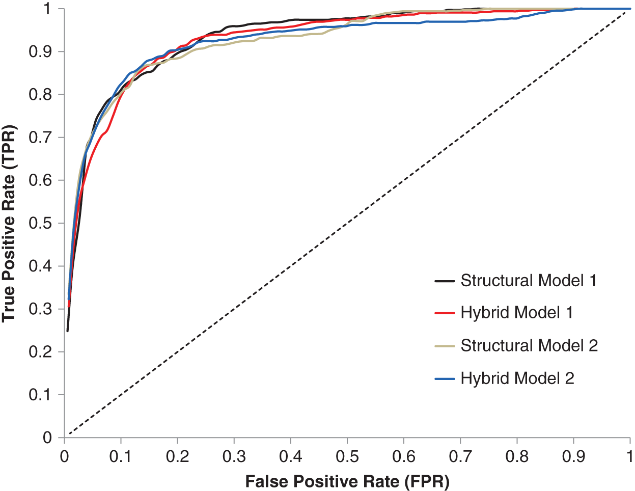
EXHIBIT 6.8 Receiver operating characteristic (ROC) curve for evaluation of four default forecasting models.
Source: Correia, Richardson, and Tuna (2012).
An added benefit of the formal analysis of default forecasts is the ancillary (see Chapter 1) nature of the test. If we can demonstrate (out‐of‐sample) skill in forecasting defaults and credit migrations, then when we see such measures are correlated with future credit excess returns, we have greater comfort about our investment process. We can forecast returns via the channel of forecasting the relevant fundamentals.
How do we use our default forecasts to generate a value measure? The simplest value measure would be the ratio of credit spreads to your default forecast (e.g., ![]() ), and then we can compare this ratio in the cross‐section (one company relative to another) or in the time series (same company relative to its own history). While this approach captures the intuition of value (a cheap corporate bond is one in which the credit spread is wide relative to your fundamental view on default risk), the ratio is limited in that it doesn't allow for controlling for other aspects of credit spreads. Generally, a type of regression (linear or otherwise) is used to link credit spreads to default forecasts and other relevant variables (e.g., recovery rates if your cross‐section has heterogeneity on the seniority dimension, or duration to capture credit curve if the cross‐section has heterogeneity on the maturity dimension). The regression residual is then the measure of “value.” Equation (6.4) is a generalization of value signals for credit sensitive assets:
), and then we can compare this ratio in the cross‐section (one company relative to another) or in the time series (same company relative to its own history). While this approach captures the intuition of value (a cheap corporate bond is one in which the credit spread is wide relative to your fundamental view on default risk), the ratio is limited in that it doesn't allow for controlling for other aspects of credit spreads. Generally, a type of regression (linear or otherwise) is used to link credit spreads to default forecasts and other relevant variables (e.g., recovery rates if your cross‐section has heterogeneity on the seniority dimension, or duration to capture credit curve if the cross‐section has heterogeneity on the maturity dimension). The regression residual is then the measure of “value.” Equation (6.4) is a generalization of value signals for credit sensitive assets:
Other than looking at future credit‐excess returns, what else might we do to convince ourselves our value measure, ![]() , is a good one? Implicit in Equation (6.4) is the notion that we have identified the component of credit spreads that is “unexplained.” If the model is well specified, this unexplained portion should be strongly mean reverting. This can be tested directly via the same statistical tests discussed in Chapter 5 (e.g., Dickey and Fuller 1979). Specifically, the following regressions can be run for each corporate issuer:
, is a good one? Implicit in Equation (6.4) is the notion that we have identified the component of credit spreads that is “unexplained.” If the model is well specified, this unexplained portion should be strongly mean reverting. This can be tested directly via the same statistical tests discussed in Chapter 5 (e.g., Dickey and Fuller 1979). Specifically, the following regressions can be run for each corporate issuer:
Equation (6.5) captures mean reversion in the value signal directly. This can be estimated over the next few (![]() ) months. For a good value measure, you will see
) months. For a good value measure, you will see ![]() , and as you cumulate across the next
, and as you cumulate across the next ![]() months,
months, ![]() , indicative of a full closure of the valuation opportunity (there is one coefficient for each of the
, indicative of a full closure of the valuation opportunity (there is one coefficient for each of the ![]() months ahead). Of course, you also need to check which “leg” of the value signal (credit spreads or your model of implied credit spreads) is converging, so you also need to see
months ahead). Of course, you also need to check which “leg” of the value signal (credit spreads or your model of implied credit spreads) is converging, so you also need to see ![]() , and
, and ![]() when estimating Equation (6.6). This is the exact approach taken in Correia, Richardson, and Tuna (2012).
when estimating Equation (6.6). This is the exact approach taken in Correia, Richardson, and Tuna (2012).
For our purposes here, we will use an equal‐weighted combination of two value measures (see e.g., Israel, Palhares, and Richardson 2018). First, we use the structural model approach from Correia, Richardson, and Tuna (2012) and regress credit spreads onto “distance of default” (![]() ) estimated as in Bharath and Shumway (2008). This can only be estimated for corporate issuers that have public equity and, as was noted at the start of the chapter, this means it cannot be estimated for a sizable minority of corporate issuers. Second, to expand coverage, we will examine a linear model based on regression residuals from a cross‐sectional regression of credit spreads onto credit ratings, spread duration, and 12‐month credit‐excess‐return volatility (this model is very similar to that used for timing credit premium in Chapter 3).
) estimated as in Bharath and Shumway (2008). This can only be estimated for corporate issuers that have public equity and, as was noted at the start of the chapter, this means it cannot be estimated for a sizable minority of corporate issuers. Second, to expand coverage, we will examine a linear model based on regression residuals from a cross‐sectional regression of credit spreads onto credit ratings, spread duration, and 12‐month credit‐excess‐return volatility (this model is very similar to that used for timing credit premium in Chapter 3).
Hang on, we have another term: distance to default (![]() ). What is this? Distance to default is central to structural models of credit, so it is important the intuition of this measure is well understood. Merton (1974) introduced the idea of distance to default to link prices of debt and equity to underlying enterprise value. Kealhofer (2003) and Correia, Richardson, and Tuna (2012) describe approaches to measure
). What is this? Distance to default is central to structural models of credit, so it is important the intuition of this measure is well understood. Merton (1974) introduced the idea of distance to default to link prices of debt and equity to underlying enterprise value. Kealhofer (2003) and Correia, Richardson, and Tuna (2012) describe approaches to measure ![]() , and that is our focus here. Equation (6.7) links
, and that is our focus here. Equation (6.7) links ![]() to measurable characteristics of a firm:
to measurable characteristics of a firm:
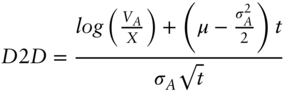
The relevant characteristics are: (i) ![]() , the market value of the enterprise (asset value as academics call it), which is simply the sum of the market value of all outstanding claims against the firm, (ii)
, the market value of the enterprise (asset value as academics call it), which is simply the sum of the market value of all outstanding claims against the firm, (ii) ![]() , the book value of the total outstanding contractual commitments the firm currently has (default barrier or threshold as academics call it), (iii)
, the book value of the total outstanding contractual commitments the firm currently has (default barrier or threshold as academics call it), (iii) ![]() , the standard deviation of the return on assets of the enterprise (asset volatility), (iv)
, the standard deviation of the return on assets of the enterprise (asset volatility), (iv) ![]() , the expected return on enterprise value due to systematic risk, and (iv)
, the expected return on enterprise value due to systematic risk, and (iv) ![]() , the remaining maturity of the contractual commitments. Let's use the visualization in Exhibit 6.9 to make the intuition clear. We are interested in quantifying the credit risk of a company that has debt and equity outstanding. On the vertical axis we measure the market value of the enterprise (asset value). This is a number. Bloomberg or Reuters or any other data vendor can provide you the data to measure this (sum up outstanding claims). Let's call this
, the remaining maturity of the contractual commitments. Let's use the visualization in Exhibit 6.9 to make the intuition clear. We are interested in quantifying the credit risk of a company that has debt and equity outstanding. On the vertical axis we measure the market value of the enterprise (asset value). This is a number. Bloomberg or Reuters or any other data vendor can provide you the data to measure this (sum up outstanding claims). Let's call this ![]() . We then read the financial statements for the company and identify all outstanding contractual commitments. This is the default barrier. Let's call it
. We then read the financial statements for the company and identify all outstanding contractual commitments. This is the default barrier. Let's call it ![]() (shown by the horizontal line labeled “Default Threshold” in Exhibit 6.9). It is clear that
(shown by the horizontal line labeled “Default Threshold” in Exhibit 6.9). It is clear that ![]() , today and the firm is not in “default” (i.e., the market value of the enterprise exceeds the total amount owed to creditors). But what we really care about is whether
, today and the firm is not in “default” (i.e., the market value of the enterprise exceeds the total amount owed to creditors). But what we really care about is whether ![]() will fall below
will fall below ![]() at some future point. I don't know that with certainty, nor do you. But we can estimate that probability, and that is what
at some future point. I don't know that with certainty, nor do you. But we can estimate that probability, and that is what ![]() is all about. The normal distribution that is turned 90 degrees in Exhibit 6.9 reflects the uncertainty with respect to what
is all about. The normal distribution that is turned 90 degrees in Exhibit 6.9 reflects the uncertainty with respect to what ![]() will be in the future. The shape of that distribution is determined by two things: (i) the average value, which is the starting value,
will be in the future. The shape of that distribution is determined by two things: (i) the average value, which is the starting value, ![]() , plus the expected return for that risky enterprise,
, plus the expected return for that risky enterprise, ![]() (drift), and (ii) the standard deviation, which is
(drift), and (ii) the standard deviation, which is ![]() (the greater the uncertainty the flatter the 90 degree rotated normal distribution). Now we have a way to think about the likelihood that
(the greater the uncertainty the flatter the 90 degree rotated normal distribution). Now we have a way to think about the likelihood that ![]() will fall below
will fall below ![]() . In Exhibit 6.9 the shaded area labeled “Default Probability” is the
. In Exhibit 6.9 the shaded area labeled “Default Probability” is the ![]() implied by Equation (6.7). This is very intuitive. The distance between the current market value of the enterprise,
implied by Equation (6.7). This is very intuitive. The distance between the current market value of the enterprise, ![]() , and current contractual commitments,
, and current contractual commitments, ![]() , is scaled by a measure of volatility,
, is scaled by a measure of volatility, ![]() , that reflects the uncertainty of the business model (the drift adjustment in the numerator and the
, that reflects the uncertainty of the business model (the drift adjustment in the numerator and the ![]() adjustment in the denominator allow comparisons across issuers with differing systematic risk levels and debt maturity profiles).
adjustment in the denominator allow comparisons across issuers with differing systematic risk levels and debt maturity profiles). ![]() closely resembles a t‐statistic, and in our case the null hypothesis is that
closely resembles a t‐statistic, and in our case the null hypothesis is that ![]() (how big a shock in asset value, measured in standard deviation units, is needed to move the firm into default?) The inputs are also very intuitive (just remember that
(how big a shock in asset value, measured in standard deviation units, is needed to move the firm into default?) The inputs are also very intuitive (just remember that ![]() is inversely related to
is inversely related to ![]() ). All else equal, if a firm (i) increases its contractual commitments,
). All else equal, if a firm (i) increases its contractual commitments, ![]() will fall, or (ii) experiences an increase in underlying volatility,
will fall, or (ii) experiences an increase in underlying volatility, ![]() will fall. These are the essential ingredients of structural models of credit risk (i.e., leverage,
will fall. These are the essential ingredients of structural models of credit risk (i.e., leverage, ![]() , and volatility).
, and volatility).

EXHIBIT 6.9 Graphical representation of  (distance to default).
Source: Correia, Richardson, and Tuna (2012).
There is a lot of choice in measuring the components of ![]() and combining them together (see e.g., Kealhofer 2003, Correia, Richardson, and Tuna 2012, and Correia, Kang, and Richardson 2018). The final step is mapping of
and combining them together (see e.g., Kealhofer 2003, Correia, Richardson, and Tuna 2012, and Correia, Kang, and Richardson 2018). The final step is mapping of ![]() to default probability (
to default probability (![]() ). While it is possible to assume the world is normally distributed and use normal distributions to map
). While it is possible to assume the world is normally distributed and use normal distributions to map ![]() to
to ![]() , this fails to recognize that the default generating process is far from normal and firms with a low normal distribution implied
, this fails to recognize that the default generating process is far from normal and firms with a low normal distribution implied ![]() may still have an economically meaningful
may still have an economically meaningful ![]() . For example, if
. For example, if ![]() this would imply a 5 standard deviation shock in asset value is needed to move a firm into default. In the world of normal random variables, this implies a
this would imply a 5 standard deviation shock in asset value is needed to move a firm into default. In the world of normal random variables, this implies a ![]() of 0.00015 percent (hardly worth worrying about), but empirically the default rate of firms with
of 0.00015 percent (hardly worth worrying about), but empirically the default rate of firms with ![]() is considerably greater. Therefore, most active credit investors working with default model will calibrate their forecasts to actual default data. This stresses the importance of quality data access.
is considerably greater. Therefore, most active credit investors working with default model will calibrate their forecasts to actual default data. This stresses the importance of quality data access.
6.3.2 Momentum
Although both valuation and momentum investment themes for credit‐sensitive assets are about forecasting changes in credit spreads, valuation rests on credit spreads mean reverting to an expected level and momentum rests on continuation in movement of credit spreads (and other market and fundamental performance measures linked to the corporate issuer). The success of momentum depends on a combination of persistence in performance measures and the markets lagged response to these measures.
We will use the same two measures of momentum examined in Israel, Palhares, and Richardson (2018). First, we use “own” momentum defined as the trailing six‐month bond credit excess return. Issuers with higher recent credit excess returns are expected to outperform issuers with lower recent credit excess returns. Second, we use “related” momentum measured as the trailing six‐month momentum of the bond issuer's equity returns. This use of equity momentum for corporate bond investing was first written about by Kwan (1996). Issuers with higher recent stock returns are expected to outperform issuers with lower recent stock returns. Of course, equity momentum can only be computed for public corporate issuers so this measure will be missing for the private issuers that we discussed in Section 6.1. The equity momentum measure for credit markets does not skip the most recent month as is typically done for equity‐momentum investing. Why? The potential for bid‐ask bounce effects to contaminate prices across markets is less of an issue, and empirically there is no evidence of any short‐term across‐markets reversal. If anything, the more recent equity returns are more predictive in credit markets.
Although our measures of momentum are both simple and transparent, the systematic investor in credit markets can look further for relevant momentum measures. There are multiple measures of fundamental health linked directly to the company, and recent changes in expectations of these variables are all candidate measures of momentum. This could include the various forecasts of default discussed earlier in the chapter. Likewise, under the heading of “related” momentum, there are many ways to identify economically linked firms (e.g., supply‐chain linkages as done in Cohen and Frazzini 2008). Measures of momentum can be projected from economically linked firms to the corporate issuer you are evaluating. Momentum can become a very broad investment theme for systematic credit investors.
6.3.3 Carry
The investment thesis for carry in corporate bonds is identical to that for carry in government bonds. We are looking to identify the expected return from holding the asset assuming nothing happens to the credit‐risk profile of the issuer as time passes. A comprehensive measure of carry requires estimation of the credit term structure. Similar to the discussion in Chapter 5 about curve fitting through zero‐coupon bond yields, identification of an issuer‐specific credit curve requires specifying the maturity structure of credit spreads that can then be used to discount corporate bond cash flows (coupon and principal). This involves obtaining pricing data for all relevant corporate bonds and the associated terms and conditions for each bond. For the purposes of this chapter we will work with a simple measure of carry, namely, the corporate bond option adjusted spread (see, e.g., Israel, Palhares, and Richardson 2018).
6.3.4 Defensive
There are two broad, but related, themes within defensive. First, we have measures related to low‐risk where the investment thesis is to capture the higher risk‐adjusted returns from lower‐risk securities, in part due to leverage aversion within fixed income markets (see e.g., Frazzini and Pedersen 2014). We will use spread duration of the corporate bond as a measure of low risk. In credit markets, beta can be approximated by the product of spread duration and spread, or DTS (e.g., Ben Dor et al. 2007). One could use DTS as a measure of risk, and under the defensive theme seek exposure to credit‐sensitive assets with lower values of DTS. This would, however, mix two ideas as discussed in Israel, Palhares, and Richardson (2018). The first component, spread duration, our focus here, has been shown to be negatively associated with risk‐adjusted returns in multiple asset classes (see e.g., van Binsbergen and Koijen 2017). The second component, credit spread, is our measure of carry for corporate bonds. Measures of beta and/or measures of volatility based on credit excess returns therefore combine two conflicting measures that have opposite effects on expected returns. We decompose beta (DTS) into its components and seek lower spread duration here as part of the defensive theme (low risk).
The second set of measures within defensive relates to “quality.” A wide set of potential measures could be included here: (i) measures of default probability (these were used conditionally with spread in our valuation signal, but could be used unconditionally here as a part of quality), and (ii) measures of profitability and components of profitability (a vast literature has explored the efficacy of financial statement analysis to better understand the persistence of corporate profitability and that literature is directly relevant here). In this chapter we will examine only the two measures from Israel, Palhares, and Richardson (2018): (i) market leverage (preference for corporate issuers with lower levels of leverage), and (ii) gross profitability (preference for corporate issuers with higher levels of profitability).
6.4 A FRAMEWORK FOR SECURITY SELECTION OF CORPORATE BONDS (PERFORMANCE)
Let's assess how well investing based on the systematic themes could have worked. We will start with a combined universe of IG and HY bonds as described in Israel, Palhares, and Richardson (2018). In each month, one representative bond is kept for each issuer from the US IG and US HY indices described at the start of the chapter. The two universes are combined, and each issuer is ranked based on the four investment themes, both individually and in combination (equal weighted). Simple academic portfolios are constructed that are long the most attractive 20 percent of issuers each month (market capitalization weighted) and short the least attractive 20 percent of issuers each month (market capitalization weighted). It is important to stress the academic nature of these portfolios. They make no attempt to address the various implementation challenges an investor faces with credit sensitive assets (e.g., sourcing liquidity, trade size limits, position limits, risk constraints, expected transaction costs, etc.). Our purpose here is to assess whether the systematic return profile is worthy of further exploration. The implementation challenges we will discuss in Chapters 8 and 9.
Exhibit 6.10 summarizes the performance of our four investment signals (value, momentum, carry, and defensive), both individually and as an equally weighted average combination. The bottom section of the exhibit reports information about the return series (Sharpe ratios, information ratios, and correlations). Except for carry, all investment themes have attractive risk‐adjusted returns with Sharpe ratios ranging from 0.98 for momentum to 1.71 for value. The Sharpe ratios and information ratios are much higher than we saw for the analysis of government bonds (these are not implementable portfolios). The equally weighted combination is superior to any one individual theme due to the low pairwise correlations you see at the bottom of Exhibit 6.10.
EXHIBIT 6.10 Properties of corporate bond security selection investment themes (V for value, M for momentum, C for carry, D for defensive, and VMCD for an equally weighted average) for the 1997–2020 period using a combined IG and HY universe.
| V | 0.13 | 0.16 | 0.04 | −0.06 | −0.03 | −0.00 | −0.01 | −0.10 | −0.07 | 5.32% |
| 8.56 | 1.55 | 0.38 | −1.70 | −0.66 | −0.01 | −0.39 | −1.62 | −2.77 | ||
| M | 0.07 | −0.71 | −0.11 | 0.07 | −0.01 | −0.01 | 0.05 | 0.07 | −0.03 | 27.32% |
| 4.81 | −7.02 | −1.15 | 2.02 | −0.16 | −0.39 | 2.20 | 1.18 | −1.28 | ||
| C | 0.01 | 0.51 | −0.33 | 0.07 | 0.04 | 0.01 | −0.01 | −0.10 | 0.00 | 63.52% |
| 1.55 | 8.19 | −5.77 | 3.63 | 1.54 | 0.65 | −0.40 | −2.74 | −0.25 | ||
| D | 0.10 | −0.94 | −0.11 | −0.01 | 0.00 | −0.05 | −0.03 | 0.04 | −0.08 | 46.85% |
| 8.60 | −10.74 | −1.37 | −0.50 | 0.03 | −1.72 | −1.42 | 0.84 | −3.43 | ||
| VMCD | 0.17 | −0.58 | −0.26 | 0.05 | 0.02 | −0.01 | 0.01 | −0.05 | −0.08 | 17.62% |
| 12.70 | −6.05 | −2.85 | 1.51 | 0.62 | −0.34 | 0.28 | −1.01 | −3.34 | ||
| V | M | C | D | VMCD | ||||||
| V | 1 | −0.32 | 0.19 | 0.05 | 0.43 | 1.71 | 1.99 | |||
| M | 1 | −0.50 | 0.56 | 0.38 | 0.98 | 1.12 | ||||
| C | 1 | −0.51 | 0.03 | 0.09 | 0.36 | |||||
| D | 1 | 0.64 | 1.26 | 2.00 | ||||||
| VMCD | 1 | 2.42 | 2.95 |
Sources: Israel, Palhares, and Richardson (2018), ICE/BAML indices, https://mba.tuck.dartmouth.edu/pages/faculty/ken.french/data_library.html, and https://www.aqr.com/Insights/Datasets.
To assess whether security selection based on value, momentum, carry, and defensive themes are diversifying with respect to traditional market risk premia (and some well‐known factor risk premia from equity markets) we run the following regression (with all explanatory variables as defined in Chapter 5):

The top half of Exhibit 6.10 reports estimated regression coefficients and, in italics below, the corresponding t‐statistics. The value investment theme is not significantly associated with either traditional market risk premia (CP, TP, and EP), or equity style returns, with an information ratio of 1.99. Of note is the insignificant ![]() regression coefficient. This means that systematic value investing in credit markets is uncorrelated with systematic investing in equity markets. At first glance, this may be puzzling to you. Aren't we talking about identifying cheap assets (bonds or stocks) linked to companies? Surely those types of investment approaches must be similar. Not necessarily. There are multiple reasons for this. First, the credit market and the equity market, while positively correlated, are diversifying with respect to each other (we covered that in Chapter 3). Second, the set of companies where we are taking active risk in equity and credit markets are different (some companies have public equity but not debt, and some companies have public debt but no equity). Third, and perhaps most important, the measures of value are very different. As discussed earlier in the chapter, equity investing is about the long term and the equity value measures (
regression coefficient. This means that systematic value investing in credit markets is uncorrelated with systematic investing in equity markets. At first glance, this may be puzzling to you. Aren't we talking about identifying cheap assets (bonds or stocks) linked to companies? Surely those types of investment approaches must be similar. Not necessarily. There are multiple reasons for this. First, the credit market and the equity market, while positively correlated, are diversifying with respect to each other (we covered that in Chapter 3). Second, the set of companies where we are taking active risk in equity and credit markets are different (some companies have public equity but not debt, and some companies have public debt but no equity). Third, and perhaps most important, the measures of value are very different. As discussed earlier in the chapter, equity investing is about the long term and the equity value measures (![]() , where
, where ![]() is a fundamental measure extracted from the primary financial statements) are deliberately constructed to be very different from the credit value measures (
is a fundamental measure extracted from the primary financial statements) are deliberately constructed to be very different from the credit value measures (![]() ). For those who have been locked in the world of fixed income markets and have not looked at the equity markets recently (read last decade) this is a very useful result. Value‐based investing in equity markets (systematic and traditional discretionary) has been very tough over the past decade (see e.g., Israel, Laursen, and Richardson 2021).
). For those who have been locked in the world of fixed income markets and have not looked at the equity markets recently (read last decade) this is a very useful result. Value‐based investing in equity markets (systematic and traditional discretionary) has been very tough over the past decade (see e.g., Israel, Laursen, and Richardson 2021).
Momentum has an attractive Sharpe and information ratio, even though it has the expected positive association with the equity momentum factor (in this case it is a common measure across equity and credit markets, but it is still diversifying). The simple academic long‐short momentum portfolio has a strong negative correlation with the credit premium. While this creates a headwind over the sample period (the credit premium was strongly positive over this period and a signal that is short that exposure inherits a negative return as a consequence), it is the consequence of poor portfolio construction choices. A simple sort on momentum will identify better recent performers as more attractive and, all else equal, such issuers will have tighter spreads, creating the negative correlation. Better portfolio construction choices can be made to neutralize signals to traditional market risk premia (more on this in Chapter 8). Defensive also shares this strong negative correlation to credit markets (issuers with lower leverage and higher profitability tend to have lower credit spreads too). Carry has the expected positive directionality with risky markets (credit and equity) and the resulting negative loading on the term premium is a direct consequence of the strong negative stock‐bond correlation over this period (see discussion in Chapter 2).
The combination portfolio exhibits some exposure to traditional market risk premia (negative to credit premium and term premium) but they are generally muted relative to individual investment themes. The adjusted ![]() of the combined signal is 17.62 percent and the regression intercept has a test statistic of 12.7! Yes, too good to be true, but it suggests if you could implement these investment themes, they would be a powerful diversifier to an asset owner portfolio.
of the combined signal is 17.62 percent and the regression intercept has a test statistic of 12.7! Yes, too good to be true, but it suggests if you could implement these investment themes, they would be a powerful diversifier to an asset owner portfolio.
As an appetizer for what is to come in later chapters, Exhibits 6.11 and 6.12 repeat the same exercise but separate the corporate bond markets into the IG and HY universes separately and also examine a wider set of measures within each of the respective investment themes implemented in a manner consistent with some of the principles to be discussed in Chapter 8 (e.g., sector demeaning signals, beta‐neutralizing signals). Separating the IG and HY universes has at least two benefits. First, it reduces heterogeneity in risk in the cross‐section making for better (more balanced) security selection. Second, it allows for differential weighting choices to be made across investment themes where you have priors for differential performance. As we have seen earlier in this book the efficacy of momentum is stronger for riskier credit sensitive assets and the efficacy of carry is stronger for safer credit‐sensitive assets. For both the HY and IG universes, the systematic investment themes are diversifying with respect to traditional market risk premia and well‐known equity factors. The adjusted ![]() for Equation (6.8) ranges from 12 to 26 percent for HY and from 8 to 19 percent for IG. These are much lower than the
for Equation (6.8) ranges from 12 to 26 percent for HY and from 8 to 19 percent for IG. These are much lower than the ![]() reported in Exhibit 6.10 for the combined universe and simpler portfolio construction. The correlation structure across investment themes is also different, partly attributable to improved portfolio construction choices (e.g., beta‐neutralizing and sector demeaning), but also due to a wider set of measures. In both markets the combination of systematic investment signals has the promise of something very attractive.
reported in Exhibit 6.10 for the combined universe and simpler portfolio construction. The correlation structure across investment themes is also different, partly attributable to improved portfolio construction choices (e.g., beta‐neutralizing and sector demeaning), but also due to a wider set of measures. In both markets the combination of systematic investment signals has the promise of something very attractive.
EXHIBIT 6.11 Properties of corporate bond security selection investment themes (V for value, M for momentum, C for carry, D for defensive, and VMCD for an equally weighted average) for the 1997–2020 period using the US HY universe.
| V | 1.04 | −0.39 | 0.51 | −0.21 | −0.00 | −0.01 | −0.02 | 0.27 | 0.09 | 16.16% |
| 26.21 | −1.26 | 1.92 | −2.19 | −0.02 | −0.14 | −0.26 | 1.66 | 1.31 | ||
| M | 0.69 | −0.53 | −0.38 | −0.04 | 0.09 | 0.01 | 0.12 | 0.81 | 0.23 | 26.39% |
| 16.45 | −1.64 | −1.36 | −0.43 | 0.78 | 0.11 | 1.63 | 4.76 | 2.99 | ||
| C | 0.62 | 0.66 | 2.19 | −0.39 | −0.28 | 0.23 | 0.08 | −1.04 | −0.15 | 15.50% |
| 9.85 | 1.35 | 5.22 | −2.55 | −1.59 | 1.41 | 0.78 | −4.06 | −1.28 | ||
| D | 0.03 | −0.14 | −0.21 | ‐0.12 | 0.06 | 0.07 | 0.04 | 0.18 | −0.04 | 12.24% |
| 1.33 | −0.77 | −1.31 | −2.05 | 0.88 | 1.17 | 1.00 | 1.88 | −0.90 | ||
| VMCD | 1.25 | −0.25 | 1.10 | −0.31 | −0.10 | 0.10 | 0.08 | 0.07 | 0.09 | 21.01% |
| 28.47 | −0.73 | 3.76 | −2.92 | −0.80 | 0.86 | 1.05 | 0.37 | 1.17 | ||
| V | M | C | D | VMCD | ||||||
| V | 1 | 0.47 | −0.09 | 0.18 | 0.83 | 5.75 | 6.24 | |||
| M | 1 | −0.45 | 0.15 | 0.44 | 3.59 | 3.92 | ||||
| C | 1 | 0.02 | 0.38 | 2.03 | 2.35 | |||||
| D | 1 | 0.22 | 0.26 | 0.32 | ||||||
| VMCD | 1 | 6.07 | 6.78 |
Sources: Author calculations, ICE/BAML indices, https://mba.tuck.dartmouth.edu/pages/faculty/ken.french/data_library.html, and https://www.aqr.com/Insights/Datasets.
EXHIBIT 6.12 Properties of corporate bond security selection investment themes (V for value, M for momentum, C for carry, D for defensive, and VMCD for an equally weighted average) for the 1997–2020 period using the US IG universe.
| V | 1.45 | −1.20 | 1.18 | −0.36 | 0.10 | −0.27 | −0.11 | −0.13 | −0.14 | 18.53% |
| 25.90 | −2.75 | 3.16 | −2.69 | 0.62 | −1.90 | −1.17 | −0.58 | −1.35 | ||
| M | 0.43 | −0.71 | 0.59 | −0.02 | 0.00 | −0.05 | −0.02 | 0.39 | 0.03 | 19.47% |
| 12.26 | −2.62 | 2.52 | −0.18 | 0.02 | −0.51 | −0.37 | 2.74 | 0.50 | ||
| C | 1.16 | 0.72 | 1.48 | −0.28 | 0.01 | −0.38 | −0.05 | −0.48 | −0.20 | 8.64% |
| 16.45 | 1.32 | 3.15 | −1.66 | 0.05 | −2.10 | −0.38 | −1.67 | −1.52 | ||
| D | 0.03 | −0.01 | 0.08 | −0.05 | −0.02 | 0.02 | 0.03 | 0.08 | 0.09 | 8.55% |
| 1.37 | −0.08 | 0.66 | −1.18 | −0.47 | 0.47 | 1.05 | 1.05 | 2.58 | ||
| VMCD | 1.61 | −0.78 | 1.53 | −0.37 | 0.07 | −0.35 | −0.09 | −0.16 | −0.15 | 16.05% |
| 25.85 | −1.60 | 3.70 | −2.50 | 0.39 | −2.16 | −0.83 | −0.64 | −1.36 | ||
| V | M | C | D | VMCD | ||||||
| V | 1 | 0.21 | 0.77 | 0.14 | 0.96 | 5.40 | 6.17 | |||
| M | 1 | −0.12 | 0.35 | 0.31 | 2.78 | 2.92 | ||||
| C | 1 | −0.01 | 0.85 | 3.63 | 3.92 | |||||
| D | 1 | 0.17 | 0.45 | 0.33 | ||||||
| VMCD | 1 | 5.51 | 6.16 |
Sources: Author calculations, ICE/BAML indices, https://mba.tuck.dartmouth.edu/pages/faculty/ken.french/data_library.html, and https://www.aqr.com/Insights/Datasets.
6.5 EXTENSIONS
6.5.1 Why Not Size or Liquidity?
Over the years working in systematic fixed income, I have been asked why we never tried to harvest a size effect in credit markets. My answer has always been this: What does size capture? It is not obvious what size means in the credit market. Are you taking a view on the size of the enterprise (sum of all debt and equity outstanding)? Are you taking a view on the equity capitalization? Are you taking a view on the amount of debt outstanding? Is that view based on the sum of all debt outstanding or is it specific to each bond? I don't know, and given I am not the one advocating this investment theme all I can do is discuss what folks might be trying to get at when they talk about “size” as an investment factor in credit markets.
I think it could be one of two things: liquidity or leverage. If the investment view is leverage, then measure that directly. Looking at the amount of debt outstanding by an issuer in an index (preference for issuers with less debt) is an imperfect way to do this. A similar discussion occurred in Chapter 5 when we discussed the potential limitations of market capitalization weighted indices. If leverage is part of your investment view, I agree with that completely, but let's agree to call it what it is; it is part of the defensive/quality theme!
If the investment view behind a preference for smaller‐sized bonds or issuers with less debt outstanding is related to liquidity (i.e., a belief in a premium to be harvested from holding less liquid assets), then it is better to measure liquidity directly. Indeed, that is exactly what Palhares and Richardson (2019) do. Theoretically, I agree with the idea of a liquidity premium. If an investor is forced to bear the risk of uncertainty with respect to selling an asset at low cost in the future, they will rationally demand a premium from holding such an asset. A liquid asset is one that can be bought/sold at a reasonable price, in a relatively short period of time, at a reasonable cost with minimal impact on its value. Not asking for too much, are we?
Palhares and Richardson (2019), using a broad sample of US IG and US HY corporate bonds, measure liquidity in six different ways: (i) issue size (smaller bonds are perceived to be less liquid), (ii) bid‐ask spreads, BAS (bonds with wider bid‐ask spreads are less liquid), (iii) market impact, MI (bonds with a larger price impact from trading, defined as the change in price for a given trading volume, are less liquid), (iv) daily trading volume, DTV (bonds that trade in smaller dollar amounts are less liquid), (v) percentage of no‐trading days, PNT (bonds that trade on fewer days are less liquid), and (vi) time since issuance, age (older bonds may be perceived to be less liquid). Palhares and Richardson (2019) examine whether these six measures of liquidity can explain cross‐sectional variation in future credit excess returns and whether long/short portfolios designed to target the less liquid bonds generate attractive risk‐adjusted returns. What was the result? Not much.
Perhaps the easiest, and cleanest, way to assess the impact of liquidity on credit markets is to look across bonds issued by the same corporate issuer that are maximally different on each respective liquidity measure. In this way, you control for any credit risk affects of the corporate issuer, and any remaining difference in credit spreads or credit excess returns is then likely attributable to liquidity. Exhibit 6.13 summarizes the analysis on credit spreads for this within issuer design from Palhares and Richardson (2019). The first two taller bars serve as a benchmark of comparison for the average level of credit spreads (AVG) and the interquartile range (IQR). The remaining smaller bars measure the average difference in credit spreads within issuer pairs of assets (i.e., what is the difference in credit spreads between the least and most liquid bond for that issuer). If there is a liquidity premium, you would expect a positive spread difference. Exhibit 6.13 shows a generally positive result, albeit small relative to the average spread level.
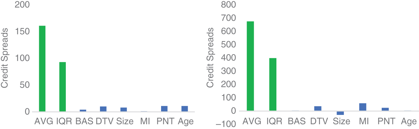
EXHIBIT 6.13 Effect of liquidity on corporate bond spreads for US IG (left) and US HY (right).
Sources: Data from Palhares and Richardson (2019), TRACE, ICE/BAML indices.
However, when looking at the difference in future credit excess returns across bonds issued by the same corporate there is no statistical evidence of a positive risk‐adjusted returns from seeking exposure to the less liquid corporate bonds. Exhibit 6.14 shows this lack of a result (all test‐statistics are below conventional levels of significance). This lack of a result, while puzzling from an academic perspective, is very important from an asset‐owner perspective. If you cannot find reliable evidence of positive risk‐adjusted returns from holding less liquid corporate bonds in an academic setting, which assumes frictionless trading, the result after incurring transaction costs and the challenge of sourcing these less liquid bonds is likely to be a negative return investment proposition. Furthermore, holding less liquid corporate bonds in an investment vehicle with frequent dealing introduces a redemption risk that seems to be uncompensated.
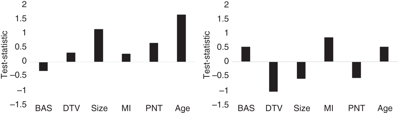
EXHIBIT 6.14 Effect of liquidity on corporate bond credit‐excess returns for US IG (left) and US HY (right).
Sources: Data from Palhares and Richardson (2019), TRACE, ICE/BAML indices.
6.5.2 Within Issuer (Maturity Dimension)
All the empirical analysis discussed in this chapter emphasized the across‐issuer dimension of security selection. Although this is the most important source of return potential, it is still possible to engage in within issuer security selection, especially for IG issuers that tend to have multiple issues outstanding. Such models will typically include measures specific to the bond rather than using corporate‐issuer‐level information (e.g., carry measures can be localized to specific points, value measures are localized to specific bonds, and other measures may naturally be unique to a bond). An added benefit of modeling multiple bonds for a given issuer is additional flexibility in portfolio construction. For example, having views on an issuer propagated across multiple bonds allows for better liquidity provision in corporate bond secondary markets. We will revisit this in more detail in Chapter 9.
6.5.3 Data Issues
A general caveat for all analysis in systematic fixed income investing is the integrity of your data. But this is especially true for credit sensitive assets. We have discussed some of these issues throughout the book, but it is worth collecting our thoughts on this topic. First, the returns data are not maintained by a central exchange and will need to be sourced directly. The most common source is from an index provider who can provide monthly (even daily) constituent‐level information on total and excess returns. Index‐provider returns are generally of high quality, but for the less liquid bonds, choices will be made to interpolate prices, or spreads, and hence returns. To help mitigate issues from poor pricing, a good systematic investment approach should source returns data from multiple sources and assess robustness across those sources. An alternative source, and one increasingly used by academics, is returns data from TRACE (trade reporting and compliance engine). Returns estimated from TRACE reported trades are problematic in several ways: (i) price‐based measures of returns are total returns, not credit‐excess returns, so they capture both rate and credit effects on corporate bonds (and we have seen earlier that these two components are negatively correlated); (ii) returns estimated from TRACE cover only a small portion of corporate bonds (especially if you require a trade at the start and end of a month); (iii) returns estimated from TRACE data are negatively serially correlated and can be predicted by index provider returns (suggesting the TRACE returns suffer from staleness issues). Andreani, Palhares, and Richardson (2022) discuss the limitations of TRACE estimated corporate bond returns.
Other important data integrity issues are related to mapping. Think of the vast array of fundamental data that needs to be mapped from a parent entity down to the entity that has issued the bond who you are thinking about buying. For some companies, the organizational structure is simple. There is one operating company with one class of stock and one type of senior unsecured debt. Alas, this is the exception. In practice, organizational forms are complicated and sometimes drastically so. Choices need to be made to link information from parent entity to issuing entity in a thoughtful manner. Not everyone agrees on how this should be done in some of the more complicated cases. As with returns, try to source multiple‐reference entity‐mapping tables to assess the robustness of your investment performance to different choices.
6.5.4 IG versus HY
As a rule, I dislike market segmentation, because it unnecessarily reduces your investment opportunity set. In corporate bond markets the extent of market segmentation is extreme. IG and HY markets are treated as separate asset classes by asset owners. This segmentation needs to be respected, which is unfortunate from an investment breadth perspective, but on the other hand it can allow tailoring of your investment themes across IG and HY markets. As we saw earlier in this chapter, momentum measures work better (worse) in HY (IG) markets and carry measures work worse (better) in HY (IG) markets. Safer corporate bonds tend to trade close to par with considerably lower spread volatility. This translates to greater spread mean reversion in IG markets, consistent with the differences in performance for momentum and carry. Take advantage of these insights in your investing. For less constrained investors, do what you can to be downgrade tolerant and expand your investment set across IG and HY markets. Even if a complete combination of IG and HY markets is a step too far, at least entertain a spillover into the neighboring rating buckets. This will allow you to avoid bad‐selling practices and improve on your security selection opportunities.
6.5.5 Sustainability/ESG
The push into sustainable investing, which started in equity markets, is gathering momentum in fixed income, especially for corporate bonds. This is an area where systematic investing approaches are uniquely positioned to be able to accommodate the joint investing challenge of delivering attractive risk‐adjusted returns but also simultaneously delivering on sustainability objectives. This topic is so vast and important that we have a later chapter dedicated to it (Chapter 10).
6.5.6 Machine Learning
I hesitate to add a subtitle with such a loaded topic. I am no expert in machine learning techniques, but I have used them successfully in the investment process. I remain skeptical of the general applicability of many of the techniques that fall under the machine learning category. There is considerable variability in the quality of investment analysis that falls under this category. One thing that seems to be generally accepted is the need for a lot of data for machine learning techniques to add value. Investing in corporate bonds does not bring with it ample trading data, so machine learning is unlikely to be helpful from a trading perspective (unlike with high frequency trading where these techniques could credibly add value, because there is very rich data at a very fine frequency). But where investing in corporate bonds may lend itself to machine learning techniques is with ancillary testing, particularly with the default forecasting models discussed earlier in the chapter as part of the valuation theme.
How might machine learning techniques be used here? There are large datasets that cover the default experience of thousands of corporates over the last 50 years. A dataset of that size lends itself to machine learning techniques. A benefit of these techniques is that they allow for consideration of a larger set of correlated forecasting variables, and the techniques also allow for potential nonlinearities and interactions among a large set of predictors.
Do these techniques help investors? Luckily, I can refer to some recent research from Correia, Kang, and Richardson (2018) that used a type of machine learning technique, random forests, to assess whether, and how, a variety of fundamental and market data could help improve out‐of‐sample forecasts of bankruptcy. Exhibit 6.15 is an example of a pruned tree that demonstrates how these techniques can improve classification of an investor‐relevant outcome (bankruptcy) using many variables in some nonobvious ways. This technique starts with all data points (68,040 firm‐year observations with a probability of bankruptcy of 0.6 percent for the entire sample) in the top box. The full sample is then partitioned using a variety of predictor variables, and the technique keeps the predictor variable that generates the maximal difference in bankruptcy probability above and below a given threshold. This generates two boxes at the first branch, which differ in bankruptcy probability by 4.8 to 0.2 percent using ![]() (a measure of leverage we discussed earlier in this chapter). The relation is intuitive: firms with more leverage (lower
(a measure of leverage we discussed earlier in this chapter). The relation is intuitive: firms with more leverage (lower ![]() ) have higher probabilities of bankruptcy. This process is repeated to generate further branches in the tree. In the second branch a measure of volatility is important (the higher the volatility the higher the risk of bankruptcy). In so doing, this tree uncovers the important interaction between leverage and volatility that is at the heart of structural models, but it does so in a data‐driven way that can identify further interactions. There is, of course, a large risk of data mining (in‐sample fitting for the politically correct reader), but that can be mitigated by cross‐validation techniques (i.e., build the tree on one set of data and assess its classification accuracy on another dataset) and randomizing across the construction of many trees (hence the name random forest). This is a promising area of future work for systematic fixed income investing.
) have higher probabilities of bankruptcy. This process is repeated to generate further branches in the tree. In the second branch a measure of volatility is important (the higher the volatility the higher the risk of bankruptcy). In so doing, this tree uncovers the important interaction between leverage and volatility that is at the heart of structural models, but it does so in a data‐driven way that can identify further interactions. There is, of course, a large risk of data mining (in‐sample fitting for the politically correct reader), but that can be mitigated by cross‐validation techniques (i.e., build the tree on one set of data and assess its classification accuracy on another dataset) and randomizing across the construction of many trees (hence the name random forest). This is a promising area of future work for systematic fixed income investing.
6.5.7 Importance of Attribution
A general challenge for systematic investors is communicating the investment narrative and explaining performance. Over the years, I have seen this done very well but also very poorly. Asset owners vary immensely in their ability and willingness to fully understand any investment process, not just systematic investment approaches. Good portfolio managers, whether they be systematic or traditional discretionary, must be able to communicate succinctly what the investment narrative is ex ante (to get the asset owner to invest), and they must be able to explain performance ex post (to retain that investment). Of course, poor performance is a reason for asset owners to redeem their investments. But failure to communicate clearly what they are doing (both ex ante and ex post) can create sufficient confusion and distrust that it may expedite that redemption risk.
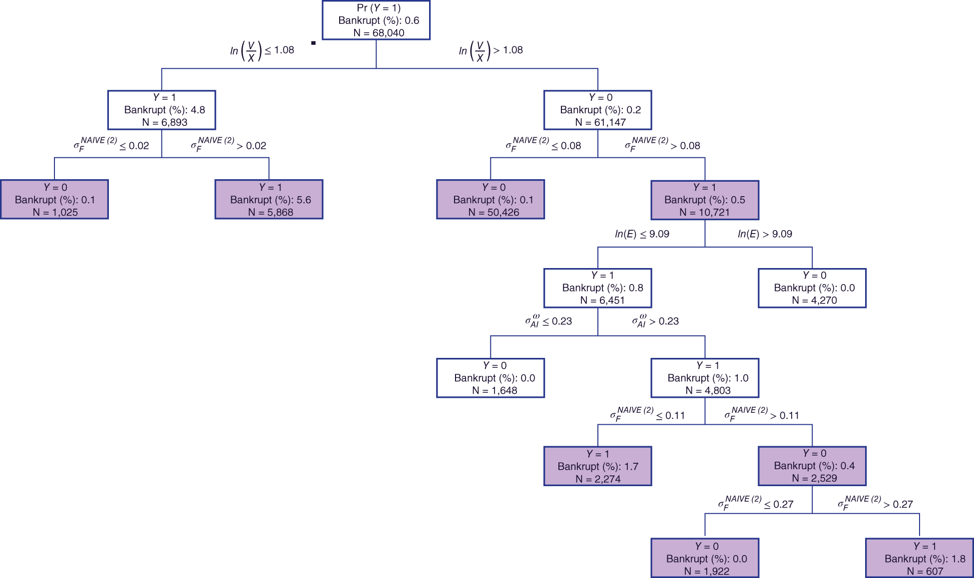
EXHIBIT 6.15 Example of a pruned tree.
Source: Based on data analysis contained within Correia, M., J. Kang, and S. Richardson. (2018). Asset volatility. Review of Accounting Studies, 23, 37–94.
So, what can/should an investor do? I am not going to provide the recipe for communication, but I cannot overemphasize how important this is and how poorly many seem to execute this dimension. Part of the asset management service is building trust and confidence with the asset owner, and this is greatly helped by a clear understanding of your investment thesis/narrative. Although a systematic manager does not, and will likely never, have a story for each bond in their portfolio, it is possible to build visual tools that allow an asset owner to look through the portfolio to the active‐risk positions and understand what the drivers are of various positions (e.g., how did your valuation measures lead to your current portfolio positioning, and how did the performance of valuation themes explain your excess of benchmark performance?) All of this, and more, is feasible with a systematic investment process. There is no right or single way to do this. It is a journey that you and your investors will need to take together.
REFERENCES
- Altman, E. (1968). Financial ratios, discriminant analysis and the prediction of corporate bankruptcy. Journal of Finance, 23, 589–609.
- Andreani, M., D. Palhares, and S. Richardson. (2022). Computing corporate bond returns form TRACE: A word (or two) of caution. Working paper.
- Arora, N., S. Richardson, and I. Tuna. (2014). Asset reliability and security prices: Evidence from credit markets. Review of Accounting Studies, 19, 363–295.
- Beaver, W. H. (1966). Financial ratios as predictors of bankruptcy. Journal of Accounting Research, 4, 71–111.
- Beaver, W. H., M. Correia, and M. McNichols. (2012). Do differences in financial reporting attributes impair the predictive ability of financial ratios for bankruptcy? Review of Accounting Studies, 17, 969–1010.
- Ben Dor, A., L. Dynkin, J. Hyman, P. Houweling, E. Van Leeuwen, and O. Penniga. (2007). DTS (Duration Times Spread). Journal of Portfolio Management, 33, 77–100.
- Bharath, S., and T. Shumway. (2008). Forecasting default with the Merton Distance‐to‐Default Model. Review of Financial Studies, 21, 1339–1369.
- Binsbergen, J., and R. Koijen. (2017). The term structure of returns: Facts and theory. Journal of Financial Economics, 124, 1–21.
- Cohen, L., and A. Frazzini. (2008). Economic links and predictable returns. Journal of Finance, 63, 1977–2011.
- Correia, M., J. Kang, and S. Richardson. (2018). Asset volatility. Review of Accounting Studies, 23, 37–94.
- Correia, M., S. Richardson, and I. Tuna. (2012). Value investing in credit markets. Review of Accounting Studies, 17, 572–609.
- Dickey, D., and W. Fuller. (1979). Distribution of the estimators for autoregressive time series with a unit root. Journal of the American Statistical Association, 74, 427–431.
- Frazzini, A., and L. Pedersen. (2014). Betting against beta. Journal of Financial Economics, 111, 1–25.
- Ilmanen, I. (2011). Expected Returns. Wiley.
- Israel, R., K. Laursen, and S. Richardson. (2021). Is (systematic) value investing dead? Journal of Portfolio Management, 47, 38–62.
- Israel, R., D. Palhares, and S. Richardson. (2018). Common factors in corporate bond returns. Journal of Investment Management, 16, 17–46.
- Kealhofer, S. (2003). Quantifying credit risk II: Debt valuation. Financial Analysts Journal, 59, 78–92.
- Kwan, S. H. (1996). Firm‐specific information and the correlation between individual stocks and bonds. Journal of Financial Economics, 40, 63–80.
- Lok, S., and S. Richardson. (2011). Credit markets and financial information. Review of Accounting Studies, 16, 487–500.
- Merton, R. (1974). On the pricing of corporate debt: The risk structure of interest rates. Journal of Finance, 29, 449–470.
- Ohlson, J. (1980). Financial ratios and the probabilistic prediction of bankruptcy. Journal of Accounting Research, 18, 109–131.
- Palhares, D., and S. Richardson. (2019). (Il)liquidity premium in credit markets: A myth? Journal of Fixed Income, 28, 5–23.
- Penman, S. (2001). Financial Statement Analysis and Security Valuation. McGraw‐Hill Irwin.
- Penman, S., F. Reggiani, S. Richardson, and I. Tuna. (2018). A framework for identifying accounting characteristics for asset pricing models, with an evaluation of book‐to‐price. European Financial Management, 24, 488–520.