
CHAPTER 5
Security Selection – Rate‐Sensitive Assets
OVERVIEW
This chapter lays out the investment opportunity set for rate‐sensitive assets. Our focus is on developed market government bonds, but the insights we cover can also be extended to emerging market government bonds. What seems like a daunting investment challenge spanning over 1,000 bonds can be distilled to a manageable set of well‐defined maturity buckets across developed markets. We cover use of principal components to help focus our scarce investment resources. Success in modeling the level, slope, and curvature (which can be achieved with as few as three assets for each country) will capture most of the return opportunities for government bonds. The chapter then discusses the intuition behind representative measures of value, momentum, carry, and defensive investment themes and evaluates the success of these strategies individually and in combination for developed government bond markets.
5.1 WHAT IS THE INVESTMENT OPPORTUNITY SET FOR DEVELOPED MARKET GOVERNMENT BONDS?
We will use a representative broad government bond index to explore our investment opportunity set. The ICE/BAML Global Government Index (W0G1) is our index of choice. W0G1 tracks the performance of publicly issued investment grade sovereign debt denominated in the issuer's own domestic currency. To be included in the index, a country must (i) be a member of the FX‐G10 or Western Europe, (ii) have an investment grade foreign currency long‐term sovereign debt rating (based on an average of Moody's, S&P and Fitch), (iii) have at $50 ($25) billion USD equivalent outstanding face value of Index qualifying debt to enter (remain in) the index, (iv) must be available to foreign investors; and (vi) must have at least one readily available, transparent price source for its underlying securities. The set of countries includes all Euro members, US, Japan, UK, Canada, Australia, New Zealand, Switzerland, Norway, and Sweden. As with most indices, W0G1 is market‐capitalization weighted. To be included, each bond must have an issue size more than $1 billion USD or (rough) equivalent, have a fixed coupon schedule, and have at least 18 months to final maturity.
Let's look at the size and composition of the W0G1 index. Exhibit 5.1 shows the market capitalization of the index over the 1996–2020 period and breaks this down across the 10 largest sovereign issuers (United States, Japan, UK, France, Italy, Germany, Spain, Belgium, Canada, and Netherlands) as of the end of the period. The total market capitalization of global government bonds is nearly $35 trillion USD and has grown substantially over the last two decades from around $7 trillion in 2000. The United States and Japan are the largest sovereign issuers accounting for 39 and 25 percent of the current $35 trillion, respectively.
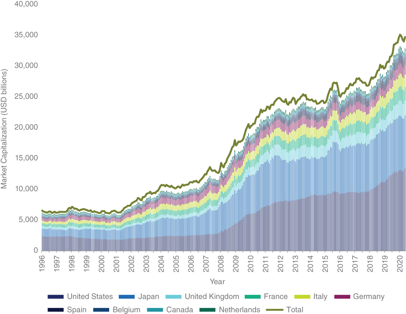
EXHIBIT 5.1 Market capitalization of ICE/BAML Global Government Bond (W0G1) index over 1996–2020 period.
Source: ICE/BAML indices.
The $35 trillion USD index as of December 2020 is made up of 1,087 bonds from 24 sovereign issuers. This looks like a very broad investment opportunity set. Exhibit 5.2 shows the number of unique issuers and number of bonds in the W0G1 index over the 1996–2020 period. Although there has been growth in the number of constituents over time, the number of issuers has remained roughly constant (and notice from Exhibit 5.1 that the largest 10 issuers account for between 90–95 percent of the total market capitalization).
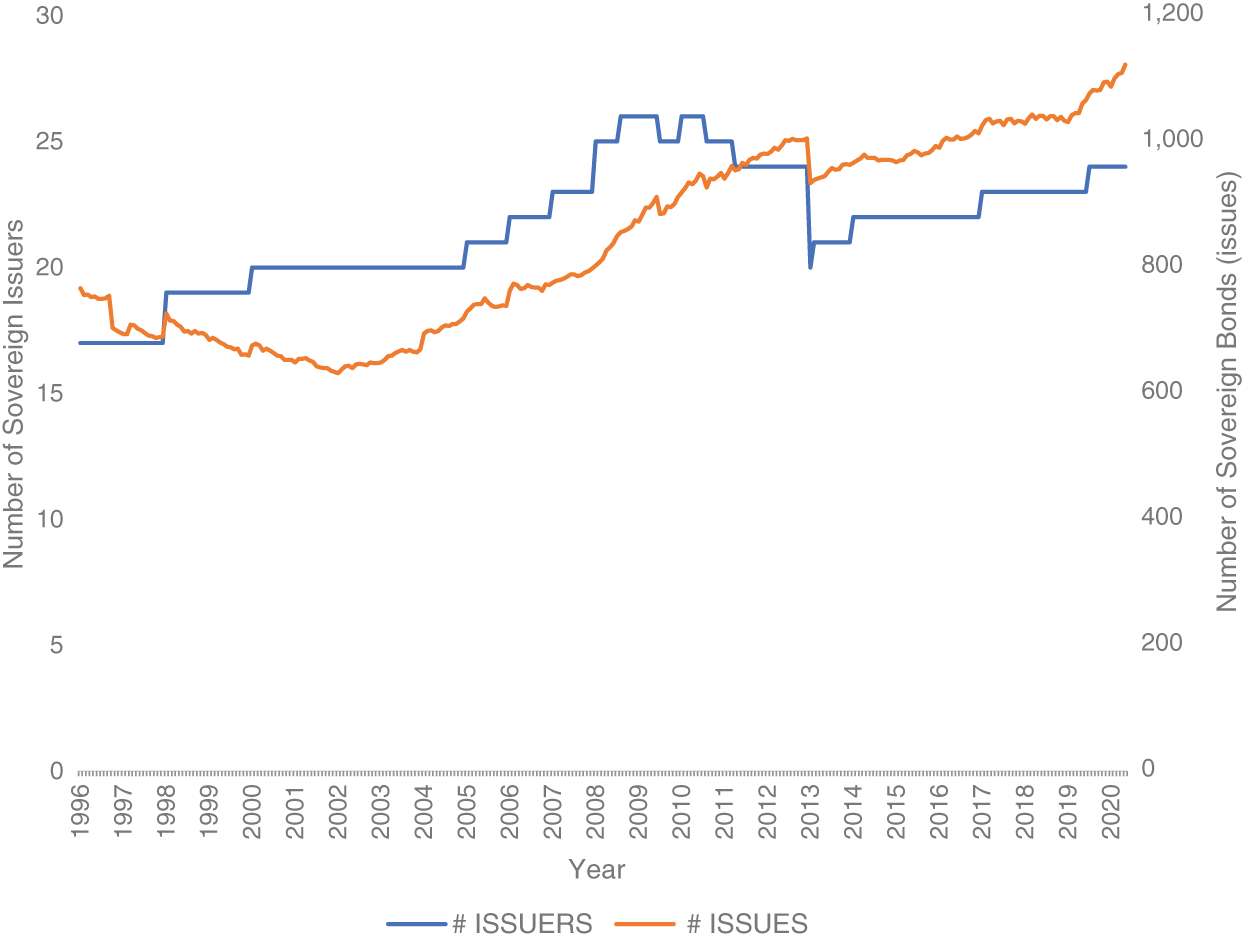
EXHIBIT 5.2 Number of unique issuers and issues in ICE/BAML Global Government Bond (W0G1) index over 1996–2020 period.
Source: ICE/BAML indices.
Another way to look at the relative concentration of rate risk across a small number of issuers is Exhibit 5.3 that shows the distribution of the number of bonds per unique issuer over the 1996–2020 period. The average (median) issuer has about 40 (20) bonds outstanding in any given month. There is considerable skew in this distribution reflecting the fact that the United States and Japan have accounted for 50–65 percent of the total market capitalization of WG01 over the 1996–2020 period, with that fraction increasing toward the end of the period.

EXHIBIT 5.3 Number of unique issues per issuer in ICE/BAML Global Government Bond (W0G1) index over 1996–2020 period.
Source: ICE/BAML indices.
So how should we be thinking about modeling expected returns and risks for this set of developed market government bonds? Do we need to be generating 1,087 individual expected return forecasts? Or is there some underlying structure in the data that might greatly simplify our forecasting exercise? As we will see, the investment opportunity set can be greatly reduced by modeling only a small number (e.g., three) of “assets” per issuer. If there are I issuers in a representative global government bond index, that means our forecasting challenge is reduced from forecasting 1,087 items to 3 × I items. Fewer than 13 sovereign issuers account for most of the market capitalization, so we are really forecasting 39 rate‐sensitive assets. How do we make the determination that three “assets” is sufficient to capture the available returns opportunity set?
5.2 REDUCING THE DIMENSIONALITY
5.2.1 Zero‐Coupon Yields and Principal Component Analysis
There is a large degree of commonality in government bond returns, as evidenced by the very high correlation of (i) government bond returns across countries for a given maturity, (ii) government bond returns across maturities for a given country, and (iii) various fixed income subsectors that share a common rates component (see, e.g., Litterman and Schienkman 1991; Brooks and Moskowitz 2017).
There are a variety of ways to identify that commonality in returns, but first, an apology. We need to introduce some mild technical discussion about principal component analysis (PCA). We will do this by way of example (and this example makes for a fun class case study). Our use of PCA is designed to do one thing: reduce the dimensionality of our return forecasting challenge. If a country (e.g., the United States or Japan) has more than 100 bonds outstanding each month (which they do), do you need to model each bond's return forecast independently? Or do they share sufficient similarity so they can be viewed as close substitutes, and you can get away with forecasting a much smaller set of bonds?
You could measure the pairwise correlation of every possible pair of bonds and then look to group bonds into clusters based on the return co‐movement patterns. This approach, although simple (perhaps cumbersome), suffers from a lack of structure. You will find a very high degree of return similarity across bonds of a given sovereign with that return similarity increasing in how close the bonds are in terms of remaining time to maturity (or duration). But this does not provide us any concrete way to reduce dimensionality.
Instead, we can use PCA. What does PCA do? PCA is a technique designed specifically to reduce the number of variables being studied while still retaining as much information as possible. That still doesn't help much. What is the information set we are looking to retain? In Chapter 2 we talked about the importance of yields in determining return potential. For government bonds, we have many bonds for each issuer. It is possible to convert the yields across a set of coupon bonds to a set of “zero‐coupon” bonds. Exhibit 5.4 shows the cash flow profile of a zero‐coupon 10‐year government bond (notice that this looks very similar to Exhibit 1.7 in Chapter 1, just without the small coupon bars). Why are we interested in zero‐coupon bonds and their yields? A zero‐coupon bond yield is simply a discount rate that can be applied to a specific cash flow (e.g., the two‐year zero‐coupon yield is the rate that is applied to convert a cash flow two years in the future to today's value). These zero‐coupon yields are an efficient way to compare bonds that share different cash flow profiles. A zero‐coupon yield is simply the internal rate of return on a cash flow with a fixed maturity; they are a standard way to normalize yield information, allowing for comparisons of fixed income securities with different maturities and from different issuers.
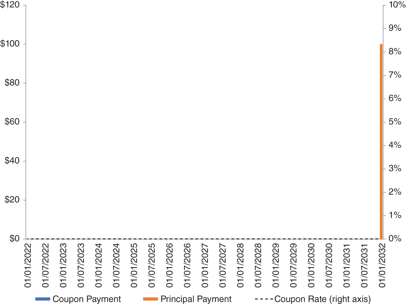
EXHIBIT 5.4 Cash flow profile of a $100 10‐year zero‐coupon bond issued on January 1, 2022.
How do we compute zero‐coupon yields? Assuming all bonds are sufficiently liquid, such that you can trust the quality of prices obtained for each bond, you have an excess of information to create zero‐coupon yields. Using simultaneous equations, you can create combinations of regular coupon bonds to create a synthetic zero‐coupon bond. How does this work? Let's use a simple example (I have used this example in class for years and it probably comes from Michael Gibbons at University of Pennsylvania Wharton School when I was an assistant professor back in the early 2000s).
Exhibit 5.5 shows the cash flows of three bonds (A, B, and C). The rows correspond to periodic cash flows. The first row is today and contains the prices of the bonds (they have negative values, as that is what you must pay to buy the bond). The next three rows capture the cash flows (coupon and par) from owning each bond. Bond A matures in three years and pays a 5 percent coupon. Bond B also matures in three years but pays a 10 percent coupon (you could think of Bond B as an off‐the‐run government bond that was issued back in time when prevailing yields were higher, but it now has a similar remaining time to maturity as Bond A). Bond C matures in two years and it has a 15 percent coupon rate. The prices of the bonds should all make sense, given they are issued by the same (risk‐free) government; the bonds with higher coupons should command a higher price.
EXHIBIT 5.5 Cash flows of three risk‐free government bonds used to create a synthetic zero‐coupon bond.
| Year | Price of Zero‐Coupon Bond | Bond A | Bond B | Bond C |
|---|---|---|---|---|
| 0 | −90.28 | −103.00 | −111.20 | |
| 1 | ? | 5 | 10 | 15 |
| 2 | ? | 5 | 10 | 115 |
| 3 | ? | 105 | 110 | 0 |
We are interested in creating a synthetic zero‐coupon one‐year bond. We would like a bond that has the following cash flows: (i) 100 in year 1, (ii) 0 in year 2, and (iii) 0 in year 3. What would be the price of such a bond? We can find a combination of the three other coupon‐bearing bonds that match these desired cash flows (i.e., we would buy ![]() units of bond A, buy
units of bond A, buy ![]() units of bond B, and buy
units of bond B, and buy ![]() units of bond C). This system of equations would be:
units of bond C). This system of equations would be:
Although we could estimate this longhand, matrix algebra helps a lot. These equations can be written in matrix form as:
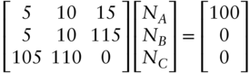
A solution to this system of equations is found by solving Equation (5.5) and Exhibit 5.6 shows the resulting positions across the three bonds that create our synthetic zero‐coupon bond. This creation of synthetic zero‐coupon bonds can continue for two‐year and three‐year zero‐coupon bonds in our example (e.g., for a two‐year zero‐coupon bond, Equation (5.4) would be modified to have  as the desired cash flows on the right‐hand side, and for a three‐year zero‐coupon bond, Equation (5.4) would be modified to have
  as the desired cash flows on the right‐hand side). Exhibit 5.6 shows the prices of all three synthetic zero‐coupon bonds, and using a simple yield formula,
 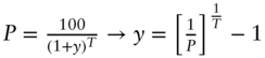 , also the corresponding zero‐coupon yields.
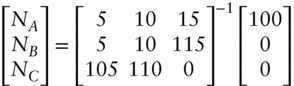
EXHIBIT 5.6 Synthetic zero‐coupon bond prices and yields for our case study of three risk‐free government bonds.
| Bond | Unit | One‐Year Zero | Two‐Year Zero | Three‐Year Zero | Price | Yield | |
|---|---|---|---|---|---|---|---|
| A | −25.3 | 3.3 | 2 | One‐year zero | −92.16 | 8.50% | |
| B | 24.15 | −3.15 | −1 | Two‐year zero | −84.67 | 8.68% | |
| C | −1 | 1 | 0 | Three‐year zero | −77.56 | 8.84% |
This example is a useful in‐class exercise for students to appreciate how zero‐coupon yields are computed. All calculations can easily be performed in Excel. Now that we know where zero‐coupon yields come from, let's look at a large dataset of zero‐coupon yields. For this we will use the dataset from Wright (2011; https://econ.jhu.edu/directory/jonathan‐wright). To save space, we will only explore US yields and focus on the period 1971–2009 using 1–10 year zero‐coupon yields. We are focused on yields as the current shape of the yield curve and future movements in the shape of the yield curve generate returns (see Chapter 1).
Our aim is to assess whether, and how, we can reduce the investment opportunity set from 10 zero‐coupon bonds to a smaller number. We will use the PCA approach described in Campbell, Lo, and MacKinlay (1996). The zero‐coupon yield dataset consists of one row for each month starting in November 1971 and ending in May 2009 (451 months) and each row contains 10 columns (one column for each year, 1 through 10). This is our [451×10] data matrix, ![]() . We will work with the natural logarithm of zero‐coupon yields (Cochrane and Piazzesi 2005) and will standardize each data series (i.e., for each zero‐coupon bond series we subtract the full‐sample mean and divide by the full sample standard deviation). The objective of PCA is to reduce the dimension from 10 to K factors (K < 10) while retaining as much of the variation in yields as possible. Principal components can be thought of as factors (linear combinations) of the 10 zero‐coupon yields. The first principal component is the linear combination of yields with the maximum variance. The second principal component is the linear combination of yields with the maximum variance that is uncorrelated to the first principal component. The third principal component is the linear combination of yields with the maximum variance that is also uncorrelated to the first and second principal components.
. We will work with the natural logarithm of zero‐coupon yields (Cochrane and Piazzesi 2005) and will standardize each data series (i.e., for each zero‐coupon bond series we subtract the full‐sample mean and divide by the full sample standard deviation). The objective of PCA is to reduce the dimension from 10 to K factors (K < 10) while retaining as much of the variation in yields as possible. Principal components can be thought of as factors (linear combinations) of the 10 zero‐coupon yields. The first principal component is the linear combination of yields with the maximum variance. The second principal component is the linear combination of yields with the maximum variance that is uncorrelated to the first principal component. The third principal component is the linear combination of yields with the maximum variance that is also uncorrelated to the first and second principal components.
Mathematically, the solution for the first principal component can be written as:
where ![]() is the linear combination of zero‐coupon yields to be solved for (a [1×10] array of weights), and Σ is the sample covariance matrix (a [10×10] matrix computed as
is the linear combination of zero‐coupon yields to be solved for (a [1×10] array of weights), and Σ is the sample covariance matrix (a [10×10] matrix computed as ![]() (the square of our standardized dataset, capturing how zero‐coupon yields at each point evolve over time individually and with each other). Subsequent principal components then have additional constraints of the type
(the square of our standardized dataset, capturing how zero‐coupon yields at each point evolve over time individually and with each other). Subsequent principal components then have additional constraints of the type ![]() (for the second component), ensuring that the factors (principal components) are orthogonal (uncorrelated) to each other.
(for the second component), ensuring that the factors (principal components) are orthogonal (uncorrelated) to each other.
Exhibit 5.7 shows the first three principal components of US zero‐coupon bond yields over the 1971–2009 period. These three principal components capture 99 percent of the total variation in zero‐coupon yields. The first (second) principal components account for 96.7 (2.9) percent of the total variation, respectively. This is the basis for reducing our investment opportunity set. Bonds share a common component that is reflected in the level of yields and common movements in the level of the yield curve account for most of the variation in yields.

EXHIBIT 5.7 First three principal components (PC1, PC2, PC3) for US zero‐coupon yields.
Source: Wright (2011).
5.2.2 Forming Maturity Bucket Assets
The first three principal components have natural interpretations (see e.g., Litterman and Scheinkman 1991). The first component is a “level” factor, the second component is a “slope” factor, and the third component is a “curvature” factor. If we link these principal components with our investment opportunity set, it will look something like this: (i) select a representative bond for each country or an average across bonds for a given country to capture the “level” factor, (ii) select a pair of bonds (buying the longer‐dated bond and shorting the short‐dated bond) to capture the “slope” factor, and (iii) selecting a triplet of bonds (buying a moderate‐duration bond and shorting both a short‐ and longer‐duration bond) to capture the “curvature” factor. Thus, with three representative bonds for a given sovereign issuer, we will be able to capture most of the variation in the yield curve and hence expected returns.
Choices need to be made for constructing the level, slope, and curvature “assets.” First, we need to select representative points across curves. A feasible approach might be to group all bonds into three buckets according to their remaining time to maturity. Brooks, Palhares, and Richardson (2018) partition bonds in each country into (i) 1–5 year (short), (ii) 5–10 year (medium), and (iii) 10–30 year (long). This will exclude bonds with a maturity greater than 30 years, but it captures most bonds in the index. Within each maturity bucket we can aggregate across all bonds by market capitalization weighting. This will generate three representative assets: short, medium, and long. Second, we need to combine these representative assets to create the assets we wish to trade (level, slope, and curvature). The level asset can be computed as the average across the short, medium, and long assets. The slope asset can be computed by buying the long asset and then shorting the short asset. The curvature asset can be computed by buying the medium asset and then shorting a combination of the short and long asset.
Our systematic investment approach is designed to capture idiosyncratic returns from security selection and not from capture of traditional market risk premia. In government bond markets, the primary risk premia is term risk, and that is linked to duration. To ensure we do not inadvertently capture term premia via our level, slope, and curvature assets, we want to “neutralize” them with respect to duration. As discussed in Chapter 1, duration is a first‐order approximation of how yield curve changes affect bonds prices, and it will leave our level, slope, and curvature assets relatively immune from general shifts in the yield curve. The level asset is already duration balanced as it (duration‐weighted) averages bonds across three maturity buckets, so selection across countries will not generate directional views on global yields.
The slope and curvature assets need to be constructed in a duration‐neutral, not dollar‐neutral, manner. This can be achieved in a variety of ways, but perhaps the simplest way to think of this is that each maturity bucket has a given duration and all returns and signals used to forecast returns can be normalized by duration (e.g., if the duration of the long maturity bucket is ![]() years and the duration of the short maturity bucket is
years and the duration of the short maturity bucket is ![]() years, then the returns for a duration neutral slope asset could be defined as
years, then the returns for a duration neutral slope asset could be defined as ![]() times the return of the long maturity bucket plus
times the return of the long maturity bucket plus ![]() times the return of the short maturity bucket). Your dataset is then ready to compare cross‐sectionally without any directional duration tilts.
times the return of the short maturity bucket). Your dataset is then ready to compare cross‐sectionally without any directional duration tilts.
In what follows, we will focus on how a systematic approach can generate outperformance via country‐level selection (we will only briefly touch on the slope and curvature assets). We will use two datasets. First, we will examine nearly a century of data on style‐based measures in fixed income (see e.g., Ilmanen, Israel, Lee, Moskowitz, and Thapar 2021). Second, we will examine a more recent dataset based on the constituents of the JPMorgan Government Bond Index (see e.g., Brooks, Palhares, and Richardson 2018). The more recent dataset has the advantage of a broader set of bonds allowing consideration of level, slope, and curvature investment possibilities. The longer dataset only allows for analysis of country‐level views but has the benefit of a much longer time series.
5.3 A FRAMEWORK FOR SECURITY SELECTION OF GOVERNMENT BONDS (INVESTMENT THEMES)
In this section we will revisit some of the well‐known investment themes discussed in Chapter 3 when we covered tactical timing decisions around the term premium. In that earlier chapter we were interested in active risk‐taking decisions in the temporal dimension (i.e., do you want to be long‐ or short‐rate sensitive assets at a given point in time). Now we are looking at active risk‐taking decisions in the cross‐sectional dimension (i.e., do you want to be long or short, or over‐ or underweight, a specific country or country‐tenor at a given point in time). These decisions (temporal vs. cross‐sectional) are directly related to each other. We are treating them as separate investment decisions, to cleanly separate market‐timing decisions (temporal) from security‐selection decisions (cross‐sectional). In Chapter 4 we saw how much of the cross‐sectional investment skill of active fixed income managers could be explained by passive exposure to traditional market risk premia. We will ex ante try to mitigate this by focusing our security selection on dimensions of attractiveness across countries that do not inherit direct exposure to duration risk. Our framework will look very similar to that discussed in Chapter 3.
5.3.1 Value
Equation (3.4) in Chapter 3 discussed how expected returns can be broken down into an initial yield (“carry”) and an expected change in yields component. Value is a type of investment idea designed to identify yields that are out of synch with underlying fundamentals that should determine the level and shape of the yield curve. Those fundamentals might include information about expected central bank monetary policy decisions, inflation expectations, economic growth, business cycle forecasts, and risk aversion. A variety of models can be used to extrapolate from current short‐term interest rates to build an expected path of future interest rates. In Exhibit 5.8, that would be the dashed black line (this is where you believe interest rates are likely to move to). The solid black line is the current zero‐coupon yield curve, the rates implied from the market pricing of government bonds. The gap between the solid and the dashed lines we can think of as our value opportunity. What does the gap represent? Ideally, it reflects that component of yield not attributable to what you have modeled (i.e., a premium component). Of course, there is always the risk of a “value trap” where market prices (yields) are aware of something that your model is missing. Therein, lies the source of risk with this type of investment signal. But that is also your opportunity as an investor: continue to refine and develop your understanding of fundamental (and nonfundamental) drivers of yields.

EXHIBIT 5.8 Visualizing value opportunities along the yield curve.
Source: Author.
For our purposes, we will use a simple measure of value for global government bonds. In the longer dataset the measure of value is taken directly from Ilmanen, Israel, Lee, Moskowitz, and Thapar (2021) as the 10‐year real bond yield. This is calculated as the difference between nominal yields and expected inflation. The measure of expected inflation here is the trailing three‐year change in the country‐specific Consumer Price Index (this ensures a consistent measure over the entire period). In the more recent dataset, we will use a measure of real bond yield that is specific to each country‐maturity bucket. This is computed as the market capitalization average yield of all bonds in the respective country‐maturity bucket less a maturity‐matched inflation‐expectation forecast from Consensus Economics. Again, note that the real bond yield is one simple way to operationalize value for rate‐sensitive assets, but there are many other possible measures.
As an aside, how do you know if your valuation measure is any good? The most obvious empirical test is to see whether your value measure (distance between where yields are compared to where you think they should be) correlates with future excess returns. Although this approach is useful, it is arguably incomplete. Future excess returns will include a component of the current yield level (“carry”). A better empirical test would be to assess whether, and how quickly, your value measure correlates with future changes in yields (see e.g., Correia, Richardson and Tuna 2012, for a similar exercise in the case of value signals for credit‐sensitive assets). Standard statistical tests (e.g., Dickey and Fuller 1979) can be used to assess the speed and magnitude of mean reversion in yields implied by your valuation signals. Further empirical analysis of non‐price‐based tests (see discussion in Chapter 1) can add comfort that your value signal is capturing the expected yield change as hypothesized. One such test might be to assess whether, and how quickly, your forecast of yield changes is reflected in the forecasts of capital market participants such as the Survey of Professional Forecasters or Consensus Economics. An ability to forecast the forecaster is valuable, because their forecasts are associated with contemporaneous changes in prices (see e.g., Bradshaw, Richardson, and Sloan 2001, who introduced this type of analysis in equity markets).
5.3.2 Momentum
Again, linking back to Equation (3.4) from Chapter 3, we can think broadly of momentum as an investment insight designed to forecast changes in yields. The general idea is that recent performance is expected to continue (return continuation is linked to behavioral biases from investors such as the disposition effect, e.g., Frazzini 2006; fundamental momentum is generally pervasive and that is not fully appreciated by capital market participants, e.g., Brooks 2017). Measures of momentum can be price‐based for the specific asset (i.e., own momentum) or based on returns of related asset classes. Despite the vast choices available to us for measuring momentum, we are going to use the simplest measure: own price momentum. Specifically, we will use the 12‐month arithmetic average of government bond excess returns. In our longer dataset, consistent with Ilmanen, Israel, Lee, Moskowitz, and Thapar (2021), the momentum measure skips the recent month's return to avoid any market microstructure effects, such as bid–ask bounce, which may induce negative short‐term autocorrelation. Given this measure is applied across countries at the 10‐year point, there is no need for further adjustments. In the more recent sample, we will use duration adjusted returns to ensure comparability in returns across maturity buckets (see e.g., Brooks, Palhares, and Richardson 2018).
It is important to remember that own price momentum is but one measure of momentum. Asset owners and investors should pay attention to the breadth of investment insights under the “momentum” label. Recent price changes of other related assets might also be useful for government bond returns. The key economic risks driving government bond yields (e.g., inflation expectations, economic growth expectations, risk aversion/sentiment) are also relevant in other assets (e.g., currencies and equities). Recent price changes from these markets may also be informative for government‐bond price changes. Similarly, the breadth of business cycle indicators that a typical fundamental analysis would look at (e.g., industrial production forecasts, inflation surveys, central bank forecast) are all relevant for the systematic investor as well. Arguably, a systematic investor is better suited to make full use of the information content across a broad set of general economic indicators. As an example of the breadth of data inputs and modeling techniques available to aggregate across a wide set of predictor variables, the interested reader can explore the popular “Nowcasting” (e.g., https://www.newyorkfed.org/research/policy/nowcast) approach, which claims to have the ability to extract information from a large quantity of data series, at different frequencies, and with different publication lags, and create a sensible view on underlying economic conditions (e.g., growth). If measured well, this can be a useful addition to a systematic investor under both the momentum and value investment themes.
5.3.3 Carry
Exhibit 3.1 provides a simple representation of what “carry” is. If nothing happens but the passage of time, carry is the return you will receive. As with our tactical timing model, we will use the term spread, ![]() , the difference in the nominal long‐term government bond yield and the nominal short‐term government yield as our measure of carry. This is an approximation for the full “carry” because it ignores curvature in the yield curve and the associated “roll‐down” component. But it has the benefit of simplicity and ease of measurement over a long period. You only need two yields (for a short‐term and long‐term bonds) to measure the term spread, whereas a comprehensive measure of carry requires multiple bonds allowing construction of the zero‐coupon yield curve we discussed earlier in this chapter.
, the difference in the nominal long‐term government bond yield and the nominal short‐term government yield as our measure of carry. This is an approximation for the full “carry” because it ignores curvature in the yield curve and the associated “roll‐down” component. But it has the benefit of simplicity and ease of measurement over a long period. You only need two yields (for a short‐term and long‐term bonds) to measure the term spread, whereas a comprehensive measure of carry requires multiple bonds allowing construction of the zero‐coupon yield curve we discussed earlier in this chapter.
A general question that students often ask around security selection for government bonds is the effect of foreign currency movements. The bonds that we are selecting from are issued in the native (local) currency of the respective sovereign (i.e., US government bonds are issued in USD, UK government bonds are issued in GBP, German sovereign bonds are issued in EUR, at least for now, and so on). We abstract away from currency effects on returns by looking at our ability to forecast excess government bond returns. The excess simply means the return of a government bond in excess of the local short‐rate (cash) instrument. The signals that we look at also abstract away from currency effects given how we measure them (e.g., momentum is based on excess returns, and our measure of carry, the term spread, is in excess of the local cash rate).
A final consideration for carry, in fact this is important for all investment signals as we will see in Chapter 8, is whether you want to volatility scale the measure or not. In the analysis that follows, we do not volatility scale any of our investment signals, but there is merit to exploring whether you want exposure to carry irrespective of the volatility of returns or whether you want your exposure to carry to be conditional on recent (or expected) volatility. There is a literature linking carry returns to episodic crashes and volatility conditioning may be a way to mitigate the episodic crashes (see e.g., Koijen, Moskowitz, Pedersen, and Vrugt 2018).
5.4 A FRAMEWORK FOR SECURITY SELECTION OF GOVERNMENT BONDS (LEVEL, SLOPE, AND CURVATURE)
5.4.1 Long Sample Evidence
Our long dataset covers the 1926–2020 period. Ilmanen, Israel, Lee, Moskowitz, and Thapar (2021) describe the full details of the dataset. The source data is the same Global Financial Data used in earlier chapters and focuses on the 10‐year bond or whatever is closest to a 10‐year bond. The cross‐section of government bonds varies through time (starting with 10 countries back in the 1920s and expanding to 28 countries by the end of the period). This analysis only considers the level asset (i.e., the security selection is simply across developed government bonds at the 10‐year point). For each investment signal (value, momentum, and carry) portfolio weights are constructed based on the strength of the signal (in Chapter 8 we will call this “signal strength weighting”). Thus, all government bonds will receive weight in the thematic portfolio, with the weight increasing in the strength of the signal. Each signal is converted to standardized ranks and these standardized ranks are the basis of portfolio weights (i.e., you will have the largest positive weight for countries with the highest rank and have the largest negative weight for countries with the lowest rank). For example, if there are three assets to choose from, you rank them 1, 2, and 3 (where 3 is the country with the strongest signal) and the average rank is 2. The weights for each asset are (1 – 2)/6, (2 – 2)/6, and (3 – 2)/6, respectively (i.e., −1, 0, +1). These weights are then rescaled to ensure a consistent notional position on the long and short side through time (i.e., avoid temporal variation in gross notional positions based on the number of assets at any one point in time). This ensures that the weights are balanced across the negative (short) and positive (long) views. This is what is commonly referred to as dollar‐neutral portfolios. It is important to note that there is no volatility scaling in these portfolios, so at each point in time the amount of risk taking in active security selection across government bonds will vary. We will come back to risk targeting in Chapter 8.
Exhibit 5.9 summarizes the performance of our three investment signals – value, momentum, and carry – both individually and as an equally weighted average combination. The bottom section of the exhibit reports information about the return series (averages, volatilities, Sharpe ratios, and correlations). The value and carry investment themes have the most attractive return profile and the equally weighted combination is superior to any one individual theme due to the low pairwise correlations you see at the bottom of Exhibit 5.9, especially the reduced volatility of the combination, which generates a much higher Sharpe ratio. The (relatively) weaker performance of momentum is consistent with the weak evidence of price momentum to help with tactical investment decisions in global government bonds (see Chapter 3).
To assess whether security selection based on value, momentum, and carry themes are diversifying with respect to traditional market risk premia (and some well‐known factor risk premia from equity markets), we run the following regression:
EXHIBIT 5.9 Properties of systematic investment themes (V for value, M for momentum, C for carry and COMBO for an equally weighted average) for global government bonds over 1926–2020 period.
| V | 0.01 | −0.01 | 0.04 | 0.01 | 0.00 | −0.00 | −0.02 | 0.96% | 0.30 |
| 2.80 | −0.23 | 1.41 | 1.54 | 0.27 | −0.50 | −1.80 | |||
| M | 0.00 | 0.00 | 0.03 | −0.00 | −0.00 | −0.00 | 0.03 | 1.14% | 0.04 |
| 0.41 | 0.03 | 1.06 | −0.44 | −0.06 | −0.40 | 2.59 | |||
| C | 0.03 | −0.02 | 0.03 | −0.01 | −0.00 | 0.00 | 0.01 | 0.88% | 0.64 |
| 5.91 | −0.70 | 1.20 | −0.70 | −1.71 | 1.19 | 1.07 | |||
| COMBO | 0.01 | −0.01 | 0.03 | 0.00 | −0.00 | 0.00 | 0.01 | 0.66% | 0.54 |
| 4.98 | −0.49 | 2.05 | 0.23 | −0.80 | 0.14 | 1.06 | |||
| V | M | C | COMBO | AVG | STDEV | ||||
| V | 1 | −0.23 | 0.28 | 0.58 | 1.35% | 4.57% | 0.30 | ||
| M | 1 | 0.07 | 0.48 | 0.50% | 4.70% | 0.11 | |||
| C | 1 | 0.74 | 2.83% | 4.35% | 0.65 | ||||
| COMBO | 1 | 1.56% | 2.71% | 0.58 |
Source: Ilmanen, Israel, Lee, Moskowitz, and Thapar (2021); data found at: https://www.aqr.com/Insights/Datasets/Century-of-Factor-Premia-Monthly. Additional factor mimicking portfolio returns found at https://mba.tuck.dartmouth.edu/pages/faculty/ken.french/data_library.html. T‐statistics reported in italics beneath regression coefficients, intercept (alpha) is annualized.
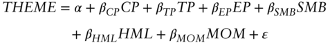
![]() is the return on the respective investment theme.
is the return on the respective investment theme. ![]() ,
, ![]() , and
, and ![]() are the credit premium, term premium and equity premium as defined in Chapter 4.
are the credit premium, term premium and equity premium as defined in Chapter 4. ![]() ,
, ![]() , and
, and ![]() are the factor‐mimicking portfolio returns based on size, value, and momentum, respectively, in the US equity market. Exhibit 5.9 reports estimated regression coefficients and, in italics below, the corresponding test‐statistics. The value and carry investment themes are not significantly associated with either traditional market risk premia (
are the factor‐mimicking portfolio returns based on size, value, and momentum, respectively, in the US equity market. Exhibit 5.9 reports estimated regression coefficients and, in italics below, the corresponding test‐statistics. The value and carry investment themes are not significantly associated with either traditional market risk premia (![]() ,
, ![]() , and
, and ![]() ), or equity style returns. The intercepts (annualized) are 1.38 percent and 2.8 percent for value and carry, respectively. Their information ratios,
), or equity style returns. The intercepts (annualized) are 1.38 percent and 2.8 percent for value and carry, respectively. Their information ratios, ![]() , are 0.30 and 0.64. An information ratio is computed as the regression intercept divided by the standard deviation of regression residuals (it is a common measure to assess the attractiveness of risk‐adjusted returns after controlling for other return sources). Momentum has an even lower
, are 0.30 and 0.64. An information ratio is computed as the regression intercept divided by the standard deviation of regression residuals (it is a common measure to assess the attractiveness of risk‐adjusted returns after controlling for other return sources). Momentum has an even lower ![]() than its standalone Sharpe ratio due to the positive exposure to the equity momentum style (there is commonality in momentum across markets as shown in Asness, Moskowitz, and Pedersen 2013). The combination portfolio exhibits some exposure to term premium (while each theme individually was only moderately exposed to term premium, the combination shares that exposure). Importantly, the regression intercept is strongly significant (1.46 percent return with a 4.98 test statistic) and the combined portfolio has a respectable
than its standalone Sharpe ratio due to the positive exposure to the equity momentum style (there is commonality in momentum across markets as shown in Asness, Moskowitz, and Pedersen 2013). The combination portfolio exhibits some exposure to term premium (while each theme individually was only moderately exposed to term premium, the combination shares that exposure). Importantly, the regression intercept is strongly significant (1.46 percent return with a 4.98 test statistic) and the combined portfolio has a respectable ![]() of 0.54. For those interested in even longer time‐series evidence of the efficacy of systematic investing for government bonds, please read Baltussen, Martens, and Penninga (2021), which contains data back to 1800!
of 0.54. For those interested in even longer time‐series evidence of the efficacy of systematic investing for government bonds, please read Baltussen, Martens, and Penninga (2021), which contains data back to 1800!
5.4.2 Recent Evidence – Level Asset
The more recent dataset uses information from the JP Morgan Government Bond Index (GBI). The analysis here was originally reported in Brooks, Palhares, and Richardson (2018), and we are now extending that data analysis up to the most recent period. The GBI is a market‐cap‐weighted index of all liquid government bonds across 13 markets (Australia, Belgium, Canada, Denmark, France, Germany, Italy, Japan, Netherlands, Spain, Sweden, the UK, and the United States). As discussed earlier, bonds are partitioned into maturity buckets: 1–5 year (short), 5–10 year (medium), and 10–30 year (long). For our country “level” asset, we form views across the 13 countries by taking an equal duration‐weighted average across the three maturity buckets within each country. Each country asset is scaled to have the same duration to remove any directional duration tilt when we rank across countries.
The country “level” views are formed by ranking across the 13 countries by each investment theme individually or in combination. Specifically, each month we form tercile portfolios of the country assets based on rankings of each theme. We form long‐short style portfolios by going long the third tercile portfolio (most attractive) and short the first tercile portfolio (least attractive) each month. Countries are equally weighted within each tercile, and all returns are in excess of the local cash rate. These portfolios are neutral to an equal parallel shift across global yield curves as they are formed in a duration‐neutral manner.
Exhibit 5.10 summarizes the performance of our three investment signals – value, momentum, and carry – both individually and as an equally weighted average combination. The bottom section of the exhibit reports information about the return series (averages, volatilities, Sharpe ratios, and correlations). All three investment themes have attractive risk‐adjusted returns with Sharpe ratios ranging from 0.31 for momentum to 0.67 for value. Again, the equally weighted combination is superior to any one individual theme due to the low pairwise correlations you see at the bottom of Exhibit 5.10, especially the negative correlation between momentum and both carry and value. Although momentum is less attractive unconditionally, it is a powerful diversifier when added to value and carry signals (value and carry are more positively correlated in the recent sample than they were over the longer time series examined earlier).
EXHIBIT 5.10 Properties of country “level” systematic investment themes (V for value, M for momentum, C for carry, and VMC for an equally weighted average) for global government bonds over 1995–2020 period.
| V | 0.02 | −0.01 | 0.07 | 0.03 | −0.00 | −0.00 | −0.00 | −0.01 | 0.01 | 3.01% |
| 2.45 | −0.22 | 1.22 | 1.71 | −0.36 | −1.06 | −0.20 | −0.35 | 0.78 | ||
| M | 0.01 | −0.05 | 0.06 | 0.03 | 0.00 | −0.00 | 0.03 | 0.02 | 0.00 | 3.30% |
| 0.83 | −0.78 | 0.94 | 1.26 | 0.50 | −0.06 | 2.07 | 0.55 | 0.10 | ||
| C | 0.02 | 0.24 | 0.08 | −0.01 | 0.00 | 0.00 | −0.01 | −0.02 | −0.01 | 10.04% |
| 2.33 | 4.06 | 1.40 | −0.70 | −1.58 | 1.56 | −0.41 | −0.66 | −0.38 | ||
| VMC | 0.02 | 0.06 | 0.07 | 0.02 | −0.00 | 0.00 | 0.01 | −0.00 | 0.00 | 4.78% |
| 3.40 | 1.77 | 2.18 | 1.44 | −0.83 | 0.25 | 0.99 | −0.24 | 0.31 | ||
| V | M | C | VMC | AVG | STD | |||||
| V | 1 | −0.29 | 0.49 | 0.71 | 2.48% | 3.72% | 0.67 | 0.55 | ||
| M | 1 | −0.36 | 0.26 | 1.25% | 4.04% | 0.31 | 0.19 | |||
| C | 1 | 0.67 | 1.91% | 3.80% | 0.50 | 0.52 | ||||
| VMC | 1 | 1.88% | 2.08% | 0.90 | 0.76 |
Sources: Brooks, Palhares, and Richardson (2018), JP Morgan Index data, Bloomberg Indices. Additional factor mimicking portfolio returns found at https://mba.tuck.dartmouth.edu/pages/faculty/ken.french/data_library.html, and https://www.aqr.com/Insights/Datasets. T‐statistics reported in italics beneath regression coefficients, intercept (alpha) is annualized.
We run a modified version of Equation (5.7) adding in two additional equity‐market factor‐mimicking portfolio returns (![]() , the betting against beta factor from Frazzini and Pedersen 2014; and
, the betting against beta factor from Frazzini and Pedersen 2014; and ![]() , the quality minus junk factor from Asness, Frazzini, and Pedersen 2019). We estimate it for the individual theme returns and the equally weighted combination, and Exhibit 5.10 reports the results. Exhibit 5.10 reports estimated regression coefficients and, in italics below, the corresponding test statistics. Consistent with the longer sample evidence, we see attractive risk‐adjusted returns for the value and carry investment themes, but we now also see attractive returns for momentum. Part of this difference is the sample period (the Sharpe ratio of momentum from the longer sample is 0.23 limiting that period to 1995–2020 vs. 0.31 shown in Exhibit 5.10) and part of it is the different cross‐section of countries examined and the weighting of all bonds across each country with positions carefully duration neutralized each month.
, the quality minus junk factor from Asness, Frazzini, and Pedersen 2019). We estimate it for the individual theme returns and the equally weighted combination, and Exhibit 5.10 reports the results. Exhibit 5.10 reports estimated regression coefficients and, in italics below, the corresponding test statistics. Consistent with the longer sample evidence, we see attractive risk‐adjusted returns for the value and carry investment themes, but we now also see attractive returns for momentum. Part of this difference is the sample period (the Sharpe ratio of momentum from the longer sample is 0.23 limiting that period to 1995–2020 vs. 0.31 shown in Exhibit 5.10) and part of it is the different cross‐section of countries examined and the weighting of all bonds across each country with positions carefully duration neutralized each month.
The combination portfolio exhibits some exposure to traditional market risk premia (![]() ,
, ![]() , and
, and ![]() ) but those exposures are modest leaving a very significant intercept of 1.55 percent and test statistic of 3.4, yielding an
) but those exposures are modest leaving a very significant intercept of 1.55 percent and test statistic of 3.4, yielding an ![]() of 0.76. These exposures to traditional beta are important to keep in mind. A criticism of incumbent active fixed income managers is that a lot of their active returns are little more than passive exposure to traditional market risk premia. We want to ensure our systematic investment approach does not also suffer from that same criticism. The results in Exhibits 5.9 and 5.10 suggest that this is not a large concern, but there is still some residual exposure. However, these portfolios are more academic in nature and do not make comprehensive use of risk modeling and exposure control tools that should be an integral part of a systematic investment process. We will return to these portfolio considerations in Chapter 8.
of 0.76. These exposures to traditional beta are important to keep in mind. A criticism of incumbent active fixed income managers is that a lot of their active returns are little more than passive exposure to traditional market risk premia. We want to ensure our systematic investment approach does not also suffer from that same criticism. The results in Exhibits 5.9 and 5.10 suggest that this is not a large concern, but there is still some residual exposure. However, these portfolios are more academic in nature and do not make comprehensive use of risk modeling and exposure control tools that should be an integral part of a systematic investment process. We will return to these portfolio considerations in Chapter 8.
5.4.3 Recent Evidence – Slope and Curvature Asset
Using the same (recent) dataset, Brooks and Moskowitz (2017) extended the analysis in Brooks, Palhares, and Richardson (2018) to explore the return performance of value, momentum, and carry signals for the country “slope” and “curvature” assets. Given the formation of country‐maturity buckets, it is relatively easy to then form duration‐balanced combinations. The “slope” asset is long the 10–30 year maturity bucket and short the 1–5 year maturity bucket. Although the bonds within each bucket are weighted on a market capitalization basis, we use a different weighting scheme when combining the maturity buckets. The slope asset is dollar imbalanced to ensure an equivalent duration exposure on the long and short side. Similarly, for the curvature asset we compute that as long the 5–10 year maturity bucket and short a combination of the 1–5 year and 10–30 year maturity buckets (the curvature asset is a net zero duration position, with the 1–5 year maturity bucket having the same duration contribution as the 10–30 year maturity bucket). Again, complete details of the construction of the slope and curvature assets can be found in Brooks and Moskowitz (2017).
Exhibits 5.11 and 5.12 report the return properties of the value, momentum and carry investment themes individually and in combination for the slope and curvature asset, respectively. For both the slope and curvature assets, value and carry have attractive risk‐adjusted returns with Sharpe ratios ranging from 0.30 to 1.08. Momentum has weaker returns, actually negative for the curvature asset. The equally weighted combination for the slope and curvature assets has a Sharpe ratio of 0.84 and 0.87, respectively. Controlling for traditional market risk premia and the broad set of equity‐style factor returns also does not reduce the attractiveness of risk‐adjusted returns, because the ![]() s are quite similar to the reported
s are quite similar to the reported ![]() s. The only notable exposure to traditional market risk premia is the positive loading that carry has to the credit premium. This is not surprising given the known episodic crash risk from carry that coincides with negative shocks to credit risk.
s. The only notable exposure to traditional market risk premia is the positive loading that carry has to the credit premium. This is not surprising given the known episodic crash risk from carry that coincides with negative shocks to credit risk.
EXHIBIT 5.11 Properties of country “slope” systematic investment themes (V for value, M for momentum, C for carry, and VMC for an equally weighted average) for global government bonds over 1995–2020 period.
| V | 0.01 | −0.04 | −0.02 | 0.02 | 0.00 | 0.00 | −0.01 | 0.02 | 0.02 | 3.59% |
| 1.33 | −0.97 | −0.67 | 1.90 | −0.80 | −0.86 | −0.60 | 0.86 | 1.91 | ||
| M | 0.01 | 0.02 | 0.04 | −0.00 | −0.00 | 0.00 | 0.00 | −0.02 | 0.00 | 1.02% |
| 1.47 | 0.43 | 0.98 | −0.22 | −0.99 | −0.55 | 0.07 | −0.93 | 0.17 | ||
| C | 0.02 | 0.13 | 0.07 | −0.00 | −0.00 | −0.00 | −0.01 | 0.02 | 0.00 | 4.65% |
| 2.54 | 2.86 | 1.68 | −0.22 | −1.41 | −1.61 | −0.55 | 0.96 | 0.07 | ||
| VMC | 0.01 | 0.04 | 0.03 | 0.01 | −0.00 | −0.00 | −0.00 | 0.01 | 0.01 | 5.15% |
| 3.32 | 1.54 | 1.32 | 0.81 | −1.99 | −1.87 | −0.65 | 0.51 | 1.25 | ||
| V | M | C | VMC | AVG | STD | |||||
| V | 1 | −0.42 | 0.04 | 0.33 | 0.96% | 2.46% | 0.39 | 0.30 | ||
| M | 1 | 0.18 | 0.51 | 0.82% | 2.71% | 0.30 | 0.33 | |||
| C | 1 | 0.77 | 1.81% | 2.73% | 0.66 | 0.57 | ||||
| VMC | 1 | 1.20% | 1.43% | 0.84 | 0.74 |
Sources: Brooks and Moskowitz (2017), JP Morgan Index data, Bloomberg Indices. Additional factor mimicking portfolio returns found at https://mba.tuck.dartmouth.edu/pages/faculty/ken.french/data_library.html, and https://www.aqr.com/Insights/Datasets. T‐statistics reported in italics beneath regression coefficients, intercept (alpha) is annualized.
EXHIBIT 5.12 Properties of country “curvature” systematic investment themes (V for value, M for momentum, C for carry and VMC for an equally weighted average) for global government bonds over 1995–2020 period.
| V | 0.01 | 0.01 | 0.02 | −0.00 | −0.00 | 0.00 | 0.00 | −0.01 | 0.00 | 3.42% |
| 3.31 | 1.21 | 1.78 | −0.63 | −1.58 | 0.00 | 0.57 | −1.88 | 0.76 | ||
| M | 0.00 | −0.02 | 0.01 | 0.00 | 0.00 | 0.00 | 0.00 | 0.00 | 0.00 | 1.23% |
| −1.56 | −1.47 | 0.50 | 0.84 | 0.58 | 0.48 | −0.38 | −0.36 | −0.64 | ||
| C | 0.01 | 0.03 | 0.01 | 0.00 | 0.00 | 0.00 | 0.00 | 0.00 | 0.00 | 2.11% |
| 4.89 | 2.15 | 1.96 | −0.39 | 0.03 | −0.75 | −0.45 | 0.27 | −0.04 | ||
| VMC | 0.004 | 0.01 | 0.01 | −0.00 | 0.00 | 0.00 | −0.00 | −0.00 | 0.00 | 2.63% |
| 3.92 | 1.07 | 1.94 | −0.04 | −0.47 | −0.16 | −0.22 | −1.11 | −0.02 | ||
| V | M | C | VMC | AVG | STD. | |||||
| V | 1 | −0.58 | −0.06 | 0.14 | 0.53% | 0.75% | 0.71 | 0.74 | ||
| M | 1 | 0.36 | 0.57 | −0.29% | 0.88% | −0.33 | −0.35 | |||
| C | 1 | 0.85 | 0.92% | 0.85% | 1.08 | 1.10 | ||||
| VMC | 1 | 0.39% | 0.44% | 0.87 | 0.88 |
Sources: Brooks and Moskowitz (2017), JP Morgan Index data, Bloomberg Indices. Additional factor mimicking portfolio returns found at https://mba.tuck.dartmouth.edu/pages/faculty/ken.french/data_library.html, and https://www.aqr.com/Insights/Datasets. T‐statistics reported in italics beneath regression coefficients, intercept (alpha) is annualized.
In summary, for both the longer time series and the more recent sample of bond index data, there is robust evidence of the efficacy of a systematic investment approach for security selection among developed‐market government bonds. Most important, not only may a systematic investment approach generate attractive risk‐adjusted returns, those returns are diversifying with respect to traditional market risk premia and alternative risk premia in the equity asset class. Brooks and Moskowitz (2017) and Ilmanen, Israel, Lee, Moskowitz, and Thapar (2021) examine the diversifying potential of systematic investing approaches across multiple asset classes. The empirical analysis contained in Exhibits 5.9–5.12 make for excellent in‐class exercises for readers to appreciate the choices in signal measurement, portfolio weighting, and the potential diversification benefits of a systematic approach.
5.5 EXTENSIONS
5.5.1 Selecting Which Bond to Trade
The astute reader will notice that trading the country “level,” “slope,” and “curvature” assets discussed in the previous sections may be unnecessarily complicated, as each maturity bucket consisted of all bonds within. Do you want to trade up and down an entire basket of bonds in each country‐maturity bucket when the attractiveness of that bucket changes? A simpler approach is to model country‐maturity buckets as quasi‐assets whose portfolio weights will change over time in response to your investment views. When trading toward your desired position for a given country‐maturity bucket, you need to select an actual bond to buy when that bucket is more attractive and select an actual bond to sell when that bucket is less attractive. Let's consider the buy decision. At a time to buy into a country‐maturity bucket, there will be multiple bonds available to purchase. It is wise to focus your attention on the more liquid bonds in that bucket (cheaper to trade in and out) and those bonds with a more attractive carry profile (expected return) at time of purchase. So over time, you may hold multiple bonds in each country‐maturity bucket as liquidity and expected returns evolve across bonds within that bucket. For the sell decision, this is more limited in a benchmark aware, long‐only portfolio, because you can only sell what you hold. However, a similar set of logic may apply; look to sell the bond in the relevant bucket with the least attractive carry profile and/or the oldest bond with a deteriorating liquidity profile.
5.5.2 Europe (Countries with a Shared Monetary Policy Framework)
The security selection across developed‐market government bonds treated all sovereigns within an index equally. For example, Germany, France, Italy, and Spain are all treated as independent assets to select from and the investment signals for these sovereigns share the same expected path of interest rates (European Union members, at least at time of writing). An investor may be able to improve their security‐selection efforts by decoupling the core from the periphery for European countries. This could be achieved by trading, say, Germany as a representative EU asset or trading a basket of EU countries together when comparing EU to other developed countries. If the basket option is selected, attention needs to be given to the weighting choice across EU members. Using market capitalization weights will give over 40 percent allocation to Italy and Spain. The volatility of excess returns for the peripheral European countries has been considerably higher than core EU countries over the last decade, as concerns about an EU breakup and fiscal weakness of peripheral countries intensified. An investor may think of modifying measures of value, momentum, and carry (and other signals) to explicitly model the “spread risk” giving rise to the additional yield on peripheral EU countries, rather than have simple value and carry signals push you into these peripheral countries.
5.5.3 Emerging Market (Local Currency) Sovereign Bonds
The empirical analysis in this chapter focused on developed‐market government bonds. The framework we developed is applicable to all rate‐sensitive assets, whether they be issued by developed or emerging sovereigns. Some care needs to be taken when extending the investment universe to include emerging markets. There are several topics worth highlighting.
First, simply extending the universe to include both developed and emerging markets may not be feasible. Asset owners typically have matrix approaches to asset classes and subgroups within asset classes. Emerging markets in fixed income are typically a separate allocation from core fixed income. But even for an unconstrained asset owner, care needs to be taken if combining developed and emerging markets together. Signal ideas do not always carry over cleanly (e.g., sensitivity to growth, which we will discuss shortly). But risk can be quite different across developed and emerging markets, in terms of both the magnitude of risk and the drivers of that risk. Careful attention is needed for risk modeling when there is considerable heterogeneity in the cross‐section, which would be the case if blending developed and emerging markets. We will discuss some aspects of how heterogeneity affects risk modeling in Chapter 8.
Second, the sensitivity of rates to growth is typically negative for rate‐sensitive assets. This is true for developed markets but is less true for emerging markets. Yields on emerging government bonds do share the central bank channel via which positive shocks to growth ultimately lead to interest rate hikes, but there is a more direct channel where the spread of the emerging government bond relative to a developed government bond is negatively related to the health of the country. Therefore, improvements in economic conditions for emerging countries can have an off‐setting negative affect on yields. Simply cutting and pasting a model from developed to emerging markets is not encouraged.
Third, there is no defensive or quality theme discussed in this chapter. A pure defensive theme could be expressed in developed and emerging markets via the betting against beta insight in Frazzini and Pedersen (2014). This would entail a long position in the bonds with the lowest beta and a short position in the bonds with the highest beta. This collapses to a passive steepener position (long the front end of the curve and short the long end of the curve) because duration is the primary source of risk in rate‐sensitive markets. Such a position entails the use of leverage (indeed leverage aversion is the basis for the betting against beta effect), making it less attractive in benchmark‐aware portfolios. But there is the possibility of “quality” measures to be used for country selection. Candidate measures could be reduced‐form indicators of the quality of government management such as (i) the level of inflation (lower is better), (ii) the level of government debt relative to GDP (lower is better), (iii) return‐based measures potentially reflecting the health of the underlying economy (e.g., stock returns or credit spreads on companies domiciled in that country or the local banking system), and (iv) measures of the robustness of the local economy (e.g., looking at measures of sectoral concentration in the local equity index). These quality measures do not have as much natural variation across developed markets, but they do for emerging markets, so they are worth including as part of a broad systematic model.
5.5.4 Market‐Capitalization Weighting
Over the years there has been criticism of market‐capitalization‐weighted indices, especially in fixed income. Market‐capitalization‐weighted indices have the natural benefit of (i) requiring minimal active trading decisions to replicate an index (as prices change the weights of bonds change automatically), and (ii) harnessing the (relative) efficiency of capital markets. Although markets are never perfectly efficient and active trading decisions are needed to replicate a benchmark (e.g., index inclusions/exclusions and a variety of actions by issuers that change the nature and size of outstanding bonds), market‐capitalization‐weighted indices still make a lot of sense.
The criticism for fixed income indices typically amounts to a criticism of index inclusion rules. Indices will include all bonds from an issuer that meet certain criteria. As we saw earlier in Section 5.1, for the W0G1 global government bond index from ICE/BAML, the United States and Japan account for nearly 65 percent of the total government debt outstanding in that index. This concentration of weights in the index is not limited to government indices; you also see this for corporate bond indices and equity indices, but not to the same extent where two issuers account for 65 percent of the total. Is this index concentration an issue? Some argue that it places too much weight on the issuers who have issued the most. While I would agree with the investment thesis to avoid issuers that have taken on too much debt, simply asserting that market capitalization indices fail because they don't account for debt issuance is wrong. The weights in the index are based on market prices. Given markets are reasonably efficient, concerns about excessive indebtedness or poor fiscal and monetary policy decision‐making by indebted sovereigns will be reflected in prices and hence index weights.
What could you do if you felt market capitalization weights are too concentrated? There are not many liquid alternatively weighted indices, but some approaches might include equal weighting across sovereigns or weighting based on the strength/size of the underlying economy (e.g., GDP weighting). Some investors take combinations of these approaches by blending different weighting schemes together. A benefit of these alternative weighting schemes can be the improved risk profile of the reweighted (and less concentrated) basket of government bonds. This can make for an excellent class exercise:
- Step 1: Start with the constituent information from a global government bond index; then roll up all bonds to the country level.
- Step 2: Compute weights for each country using market capitalization weights, equal weights, GDP weights, and possibly a measure inversely related to recent volatility.
- Step 3: Compute index level returns using these alternative weighting schemes.
- Step 4: Evaluate the return profile of these alternative index level returns (i.e., average returns, volatility of returns, and Sharpe ratios).
Question: Do the alternative weighting schema deliver on their promise of a “better” return profile? In what way are the return series better? Distinguish between numerator and denominator effects.
One closing thought on index weighting choices. If your investment hypothesis is to avoid issuers that are overly indebted, then bet on that directly (I agree with this investment hypothesis). Switching to an equally weighted index is not the best way to pursue that investment hypothesis. If you dislike issuers with too much outstanding debt, then measure the leverage of the issuer directly and use that as a “signal” to take active positions relative to the benchmark (or active risk generally in a hedge fund). Simply using an equally weighted benchmark in lieu of a market capitalization weighted benchmark is deficient in two key respects: (i) the magnitude of active risk (tracking error) relative to benchmark is unmodeled and may be outsized relative to your conviction, and (ii) the difference between equal and market capitalization weights reflects the size of the issuer, not leverage, so the resulting portfolio is a noisy reflection of your investment hypothesis.
REFERENCES
- Asness, C., A. Frazzini, and L. Pedersen. (2019). Quality minus junk. Review of Accounting Studies, 24, 34–112.
- Asness, C., T. Moskowitz, and L. Pedersen. (2013). Value and momentum everywhere. Journal of Finance, 68, 929–985.
- Baltussen, G., M. Martens, and O. Penninga. (2021). Factor investing in sovereign bond markets: Deep sample evidence. Journal of Portfolio Management, 48, 209–225.
- Bradshaw, M, R. Richardson, and R. Sloan. (2001). Do analysts and auditors use information in accruals? Journal of Accounting Research, 39, 45–74.
- Brooks, J. (2017). A half century of macro momentum. AQR working paper.
- Brooks, J., and T. Moskowitz. (2017). Yield curve premia. Working paper, AQR.
- Brooks, J., D. Palhares, and S. Richardson. (2018). Style investing in fixed income. Journal of Portfolio Management, 44, 127–139.
- Campbell, J., A. Lo, and C. MacKinlay. (1996). The Econometrics of Financial Markets. Princeton University Press.
- Cochrane, J., and M. Piazzesi. (2005). Bond risk premia. American Economic Review, 95, 138–160.
- Correia, M., S. Richardson, and I. Tuna. (2012). Value investing in credit markets. Review of Accounting Studies, 17, 572–609.
- Dickey, D., and W. Fuller. (1979). Distribution of the estimators for autoregressive time series with a unit root. Journal of the American Statistical Association, 74, 427–431.
- Frazzini, A. (2006). The disposition effect and underreaction to news. Journal of Finance, 61, 2017–2046.
- Frazzini, A., and L. Pedersen. (2014). Betting against beta. Journal of Financial Economics, 111, 1–25.
- Ilmanen, I., R. Israel, R. Lee, T. Moskowitz, and A. Thapar. (2021). Journal of Investment Management, 19, 15–57.
- Koijen, R., T. Moskowitz, L. Pedersen, and E. Vrugt. (2018). Carry. Journal of Financial Economics, 127, 197–225.
- Litterman, R., and J. Scheinkman. (1991). Common factors affecting bond returns. Journal of Fixed Income, 1, 54–61.
- Wright, Jonathan H. (2011). Term premia and inflation uncertainty: Empirical evidence from an international panel dataset.” American Economic Review, 101(4): 1514–1534.