
9
Current Transformers
Current transformers (CTs) enable the measurement of currents in situations where either the system voltage or the magnitude of the current is too large to permit direct measurement. The current to be measured flows in the CT primary winding (usually just a single turn) and a scaled replica flows in its secondary. Current transformers are essential components in both protection and metering circuits, and while they are rugged devices they do have some limitations.
For example, like voltage transformers, CTs introduce both magnitude and phase errors into the secondary current. While these can be made arbitrarily small for metering applications, protection CTs must operate correctly during system faults, when primary currents can reach many times their normal value. Under these conditions a CT may approach saturation, and as a result its error will inevitably increase. In addition, in this region the non‐linear magnetising characteristic will introduce a significant harmonic content into the magnetising current, making phasor analysis inapplicable.
To minimise the likelihood of saturation and to reduce the size of the magnitude and phase errors, current transformers are designed to normally operate at very low flux densities. This is achieved by imposing a restriction on the size of the secondary voltage that a CT must generate, which in turn is achieved by limiting the burden impedance that can be connected across its secondary winding. As a consequence, the VA rating of current transformers tends to be small. For example, metering class CTs rarely have ratings in excess of 30 VA, and usually considerably less than this.
The rated burden is the maximum load (expressed in either VA or ohms) that can be supported by a CT while maintaining its accuracy requirements. Any burden less than the rated can be safely applied, but overburdening a CT will generally result in an additional measurement error. The VA rating of a CT is given by the square of the rated secondary current, multiplied by the rated burden, expressed in ohms.
Because of the significant difference in performance required for protection duties as compared to metering, current transformers are usually designed either for one purpose or the other. Protection cores tend to be larger, and they therefore contain more transformer steel than their metering counterparts. This enables them to carry substantial fault currents and to support high secondary voltages, without becoming heavily saturated. Metering cores, on the other hand, are smaller and cheaper and operate over a much narrower range of currents. During fault conditions they become saturated, thereby limiting the exposure of the attached metering equipment to damaging currents.
Figure 9.1 shows a 220 kV pedestal CT, used in aerial switchyards. This type of CT can be fitted with several independent cores, either for protection or metering purposes. The CT depicted in Figure 9.2 is one of several cores that can be fitted around the bushing of a dead tank circuit breaker. It consists of a tape wound toroidal core upon which is wound the secondary winding, in this case one with three tappings.
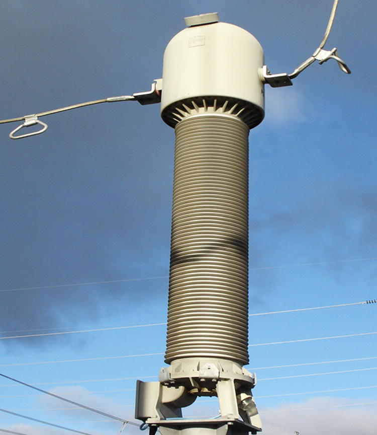
Figure 9.1 220 kV pedestal CT.

Figure 9.2 A 15 VA, Class 1, 600,400,200:5 toroidal bushing CT.
9.1 CT Secondary Currents and Ratios
Current transformers are generally designed to deliver secondary currents of either 1 A or 5 A, when operating at rated primary current, the choice of which depends to a large extent on the distance between the CT and its associated protection relay or energy meter. Where this distance is short, 5 A secondary currents are usually chosen, as is usually the case in LV metering applications. This helps to reduce the cost of the CT, albeit at the expense of requiring a lower turns ratio, which can adversely affect the magnitude and phase errors. On the other hand, for long cabling runs, the fraction of the available burden consumed by the voltage drop in the interconnecting cables can become significant, and in such cases 1 A CTs are generally used instead. Protection CTs, particularly in aerial switchyards, are therefore usually 1 A devices, although in the United States there is a preference for 5 A CTs in protection applications.
Current transformer ratios are expressed as the ratio of rated primary to secondary current, e.g. 1000:1 for a 1 A CT or 1000:5 for a 5 A device. Frequently, tappings are included on the secondary winding so as to provide multiple current ratios from the same CT. For example, the ratio of a three tap CT will usually be expressed in the form 1000, 800, 400:5. Tappings enable the ratio to be altered as load growth occurs, and provide a choice of ratio in protection applications, without the need to physically change the CT.
9.1.1 CT Terminal Labelling Convention and Connection Arrangements
The terminals of a current transformer are always clearly marked since the correct phasing of current transformers is critical in both protection and metering applications. The CT primary terminals are marked P1 and P2, usually on the case of the device, as are the corresponding secondary terminals, S1 and S2. Figure 9.3a shows that a primary current flowing from P1 to P2 generates a proportional secondary current flowing from S1 to S2. In the case of multi‐tap CTs, the secondary terminals are labelled progressively S1, S2, S3 … Sn, from the common end of the secondary winding (S1), to the highest tapping (Sn).

Figure 9.3 (a) Four wire connection (b) Residual current connection.
In order to further reduce the cabling burden imposed on a CT, it is common to star connect the secondary terminals at the CT marshalling enclosure, and again at the burdening device, as shown in Figure 9.3a. This permits one side of each secondary winding to be earthed, and requires only four wires to deliver the current information to the associated instrumentation. In the case of three‐wire MV or HV circuits, the primary phase currents will sum to zero and thus the current in the neutral wire will also be zero. This roughly halves the cabling burden seen by each CT. This approach is generally adopted where long cable runs are necessary.
In four‐wire MV or LV circuits, where the load is balanced or approximately so, a similar benefit will also exist, since the neutral wire will only carry the residual current. For unbalanced loads the burden seen by the CTs will generally be larger, since the voltage drop in the neutral must also be supported by each CT.
The residual connection of Figure 9.3b is frequently used to isolate the zero‐sequence current from a set of three‐phase currents. Each CT generates all three sequence components in its secondary current, but being balanced, the positive and negative sequence currents add to zero in the summation, leaving three times the zero‐sequence component flowing in the burden.
9.2 Current Transformer Errors and Standards
Like voltage transformers, current transformers also introduce small magnitude and phase errors into their secondary currents. These arise due to the need for a magnetising current to generate sufficient flux density to produce the voltage demanded by the burden. Since the magnetising current is consumed internally, the current seen by the burden differs slightly in both magnitude and phase from that which might otherwise be expected. In addition, the magnetising impedance is not constant, but instead depends on the flux density that the CT is called upon to support in order to circulate secondary current through the burden. Therefore both the applied burden and the actual secondary current, influence the CT errors.
As mentioned above, current transformers may saturate during fault conditions when large currents flow. Metering CTs are designed to saturate under such conditions, but protection CTs must be dimensioned to operate correctly throughout network faults, without becoming heavily saturated. As a result, a significant performance difference exists between the two, and their characteristics are separately defined in current transformer standards.
We will again confine our general interest in current transformer standards to two documents. The first is the European standard IEC61869‐2 Additional Requirements for Current Transformers and the second is the same American standard that also applies to voltage transformers, IEEE C57.13 IEEE Standard Requirements for Instrument Transformers, together with its supplement, IEEE C57.13.6 IEEE Standard for High‐Accuracy Instrument Transformers.
However, there are two additional standards to consider in the specification of current transformers associated with protective relaying. The first is the European standard IEC61869‐1 General Requirements for Instrument Transformers and the second is the American standard IEEE C37.110 IEEE Guide for the Application of Current Transformers used for Protective Relaying Purposes.
9.2.1 Current Transformer Magnitude and Phase Errors
Current transformers introduce errors into their representation of the primary current, in much the same way as voltage transformers introduce errors into their representation of primary voltage. In the case of current transformers, magnitude and phase errors arise as a result of the magnetising current required to generate the flux required in the core.
The magnitude (or ratio) error (e) of a current transformer is “the error in the magnitude of the fundamental component of the actual secondary current when a sinusoidal current flows in the primary” (AS1675, 1986). It can be expressed as:

where N is the rated transformation ratio, Ip is the actual primary current and Is is the actual secondary current.
The phase error β, is the difference in phase between the primary current phasor and the secondary current phasor. The phase error is defined as positive when the secondary current phasor leads that of the primary. It is measured in minutes of arc (Min) or in centiradians (Crad) where 1 Crad = 0.01 radian = 34.4 Min.
9.2.2 IEC 61869‐2 Metering Class Magnitude and Phase Errors
IEC 61869‐2 prescribes eight standard accuracy classes for measuring current transformers: 0.1, 0.2, 0.2S, 0.5, 0.5S, 1, 3 and 5. Class 0.1 applies to laboratory grade instruments, while classes 0.2–1 are used in revenue metering applications, and classes 3 and 5 are for non‐critical applications such as panel instrumentation.
Table 9.1 outlines the error limits for classes 0.1–1, as prescribed under IEC 61869‐2. Since current transformer errors are a function of the secondary voltage, both the secondary current and the applied burden must be specified when defining the error limits. The standard specifies a burden power factor (pf) of 0.8, which means that the rated burden includes both resistive and inductive elements. This is not to say that a compliant CT must always be so burdened, but rather that error testing must be done with a 0.8 pf burden.
Table 9.1 Metering class error limits.
(IEC 61869‐2 ed.1.0 Copyright © 2012 IEC Geneva, Switzerland. www.iec.ch)
| Magnitude error (±%) | Phase error (±Crad) | |||||||
| Primary current (%) | Primary current (%) | |||||||
| Accuracy class | 5 | 20 | 100 | 120 | 5 | 20 | 100 | 120 |
| 0.1 | 0.40 | 0.20 | 0.10 | 0.10 | 0.45 | 0.24 | 0.15 | 0.15 |
| 0.2 | 0.75 | 0.35 | 0.20 | 0.20 | 0.90 | 0.45 | 0.30 | 0.30 |
| 0.5 | 1.50 | 0.75 | 0.50 | 0.50 | 2.70 | 1.35 | 0.90 | 0.90 |
| 1 | 3.00 | 1.50 | 1.00 | 1.00 | 5.40 | 2.70 | 1.80 | 1.80 |
The standard also requires that a CT be compliant between 25% to 100% of its rated burden, at 5, 20, 100 and 120% of rated current. Manufacturers generally error test their CTs at 25% and 100% of the rated burden, at each specified percentage of rated primary current. It can be seen from the table that the error limits are considerably more relaxed at small primary currents, i.e. where both the secondary current and voltage are also small. The reason for this will become apparent in Section 9.5.
As shown in Table 9.2, class 0.2S and 0.5S transformers (sometimes called special class CTs), must maintain the prescribed error for currents as small as 1% of the primary rating. They must also achieve their ultimate error limits by 20% of rated current.
Table 9.2 Metering class error limits for class 0.2S and 0.5S CTs.
(IEC 61869‐2 ed.1.0 Copyright © 2012 IEC Geneva, Switzerland. www.iec.ch)
| Magnitude error (±%) | Phase error (±Crad) | |||||||||
| Primary current (%) | Primary current (%) | |||||||||
| Accuracy class | 1 | 5 | 20 | 100 | 120 | 5 | 10 | 20 | 100 | 120 |
| 0.2S | 0.75 | 0.35 | 0.20 | 0.20 | 0.20 | 0.90 | 0.45 | 0.30 | 0.30 | 0.30 |
| 0.5S | 1.5 | 0.75 | 0.50 | 0.50 | 0.50 | 2.70 | 1.35 | 0.90 | 0.90 | 0.90 |
In the case of multi‐tap CTs, the higher ratios will generally offer improved accuracy, since the core excitation is proportional to the ampere‐turns applied. With more secondary turns available, less magnetising current is required to achieve a given flux density, and therefore the errors introduced into the secondary current reduce accordingly. For example, it is possible that the multi‐tap metering CTs in Figure 9.4 may satisfy the 0.5 class requirements on the 1000:1 tap and the 0.2 class on the 3000:1 tap. The appropriate accuracy class will always be stated for the lowest tap, and may sometimes be stated for higher taps as well.

Figure 9.4 Busbar mounted multi‐tap metering CTs (3000, 2000, 1000:5, 15 VA).
9.2.3 IEC 61869‐2 Metering Class Burdens and Extended Range Operation
The rated burden is the load, usually expressed in VA or in ohms, which a CT can supply while maintaining its prescribed accuracy, at rated primary current. For example, a 1000:1 15 VA CT can support a maximum burden impedance of ![]() ohms, whereas for a 1000:5, 15 VA transformer, the burden is limited to
ohms, whereas for a 1000:5, 15 VA transformer, the burden is limited to ![]() ohms.
ohms.
IEC 61869‐2 defines a range of standard burdens for metering class CTs, specifically 2.5, 5, 10, 15 and 30 VA. In many LV metering applications the current transformers are located close to the energy meter, and in such cases CTs with a relatively small rated burden can be chosen, 5 VA being typical. However, in HV protection applications, particularly in aerial switchyards where the route length of the secondary cables is long, larger CT burdens will generally be specified. This will avoid the need to install long lengths of heavy secondary cable.
9.2.4 Extended Range CTs
IEC 61869‐2 also permits the use of extended current ratings for metering class CTs with accuracy classes between 0.1 and 1. Tables 9.1 and 9.2 show that a standard metering CT is class compliant up to 120% of its rated primary current. This means that the magnitude and phase errors prescribed for 100% of rated current must also apply at 120%. Extended range CTs are similarly class compliant, but to a higher multiple of rated current, possibly as high as 200% or 250%. It is also a requirement that the continuous thermal rating current for the CT equals or exceeds the extended range primary current.
Extended range CTs are frequently used in LV metering applications, where they enable a wide range of currents to be accommodated within a particular accuracy class. For example, an 800:5 class 0.5 CT, with an extended range of 250% is class compliant from 40 A through to 2000 A. The use of such CTs avoids the need to change tappings as load growth occurs, and enables a considerably smaller range of CTs to be held in stock for LV applications.
9.3 IEEE C57.13 Metering Class Magnitude and Phase Errors
The American standard IEEE C57.13 defines three standard accuracy classes of metering transformer (0.3, 0.6 and 1.2) and its supplement, IEEE C57‐13.6, defines two additional high accuracy classes, 0.15 and 0.15S. As with voltage transformers, this standard does not directly prescribe magnitude and phase errors, instead it places limits on the transformer correction factor (TCF).
As is the case with voltage transformers, any magnitude or phase errors inherent in a current transformer will introduce a small error into the measurement of the power or energy by a metering installation. This error may be corrected using the TCF, which relates the measured power (Pmeasured) to the correct power (Pcorrect), according to:

The TCF may be calculated from the ratio correction factor (RCF), the phase error β and the phase angle of the metered load ϕ, according to:

(Note that this equation does not include the errors associated with the voltage transformers also used in the metering installation.)
The RCF for a current transformer is defined in a similar way to that for a voltage transformer. It is the factor by which the stated ratio of an instrument transformer must be multiplied to obtain the actual ratio. Therefore the RCF can be used to correct the current measured by a CT for the effects of magnitude error:

where |Imeasured| is the magnitude of current measured by the CT in question, and |Icorrect| is this quantity corrected for the ratio error introduced by the CT.
IEEE C57.13 prescribes limits on the TCF for accuracy classes 0.3–1.2, which appear in Table 9.3. Those prescribed by IEEE C57.13.6 apply to classes 0.15 and 0.15S and appear in Table 9.4. These limits must be maintained from 0% to 100% of the transformer’s rated burden and for metered loads with lagging power factors between 0.6 and 1.0. The limits applicable to rated current must also be maintained up to the continuous thermal current rating of the device, which effectively gives the CT an extended operating range.
Table 9.3 Accuracy class limits for metering classes 0.3–1.2.
(Adapted and reprinted with permission from IEEE. Copyright IEEE C57.13 (2008) All rights reserved. Permission for further use of this material must be obtained from IEEE. Requests may be sent to stds‐[email protected])
| Transformer correction factor (TCF) | ||||
| At 100% rated current | At 10% rated current | |||
| Accuracy class | Minimum | Maximum | Minimum | Maximum |
| 0.3 | 0.997 | 1.003 | 0.994 | 1.006 |
| 0.6 | 0.994 | 1.006 | 0.988 | 1.012 |
| 1.2 | 0.988 | 1.012 | 0.976 | 1.024 |
Table 9.4 Accuracy class limits for metering classes 0.15 and 0.15S.
(Adapted and reprinted with permission from IEEE. Copyright IEEE C57.13.6 (2010) All rights reserved. Permission for further use of this material must be obtained from IEEE. Requests may be sent to stds‐[email protected])
| Transformer correction factor (TCF) | ||||
| At 100% rated current | At 5% rated current | |||
| Accuracy class | Minimum | Maximum | Minimum | Maximum |
| 0.15 | 0.9985 | 1.0015 | 0.9970 | 1.0030 |
| 0.15S | 0.9985 | 1.0015 | 0.9985 | 1.0015 |
Prescribing limits applicable to the TCF, indirectly places limits on both the RCF and the phase error of a CT. The TCF is largest when the power factor of the metered load the lies at the lower end of the permitted range, i.e. when it equals 0.6. Under these conditions Equation (9.3) defines the relationship between these parameters. (This equation is fully discussed in Chapter 10.)
As a result, the ratio correction factor and the phase error are no longer independent of each other, and instead are constrained to lie within the parallelogram appropriate to the class of the CT, shown in Figure 9.5.

Figure 9.5 Current transformer limits of accuracy as prescribed by IEEE C57.13.
(Adapted and reprinted with permission from IEEE. Copyright IEEE C57.13 (2008) All rights reserved. Permission for further use of this material must be obtained from IEEE. Requests may be sent to stds‐[email protected]).
9.3.1 Error Comparison between IEC 61869‐2 and IEE C57.13
The total error (or overall error) is a scalar figure of merit for a CT, which embodies both magnitude and phase error information in the measurement of the power flow to a load. It is related to the TCF according to:

So if the TCF is 0.995, the total error will be +0.5%.
A graphical comparison between the total error of two current transformers as a function the percentage of primary current appears in Figure 9.6. One of these is a 0.2 class device, compliant with the European Standard IEC 61869‐2, while the other is a 0.3 class CT, compliant with IEEE C57.13. Although the nomenclature suggests otherwise, an inspection reveals that the performance of the 0.3 class device is superior to that of the 0.2 class. This is because both the magnitude and phase errors are interdependent in the case of the 0.3 class CT, whereas they are not so constrained in the specification of the 0.2 class CT.

Figure 9.6 Comparison of CT specifications (primary circuit pf = 0.6).
9.4 Current Transformer Equivalent Circuit
Current transformer magnitude and phase errors can be shown to be related to components of the CT equivalent circuit. In particular, both these errors depend to a large extent on the value of the magnetising current Im.
Consider the equivalent circuit shown in Figure 9.7. The CT on the left is an ideal current transformer, i.e. one requiring no magnetising current. In parallel with its secondary winding is an admittance ![]() , through which flows the magnetising current Im demanded by a real CT. Provided the CT is not operated near saturation, this admittance is considerably smaller than that of the burden, and therefore the CT errors will be quite small.
, through which flows the magnetising current Im demanded by a real CT. Provided the CT is not operated near saturation, this admittance is considerably smaller than that of the burden, and therefore the CT errors will be quite small.

Figure 9.7 CT equivalent circuit.
Note that Nact in the figure above is the actual turns ratio used, which may be slightly different from the nominal ratio N in the case where turns compensation (see Section 9.5.2) has been applied. (In cases where n1 equals one turn, Nact equals n2.)
Unlike voltage transformers, the leakage inductance associated with a toroidal CT is generally negligible. This is particularly so if the primary consists of a single turn, centred in a toroidal core with a uniformly distributed secondary winding, and the magnetic effects of the return primary conductor, or those of the other phases, are negligible. Therefore the only series element to be considered is the secondary winding resistance Rct.
In general, the burden connected to the CT can be represented by a series connected resistance and inductance (Rb + jXb). The secondary voltage generated by the CT, Vs, is that developed across the magnetising admittance. Since this is also the voltage applied to the series connection of the winding resistance and the burden, it is convenient to associate these elements, therefore we write ![]() .
.
We use an admittance approach in the evaluation of CT errors, since it provides both a simpler analysis and error equations closely analogous to Equations 8.4 and 8.5, previously derived for voltage transformer errors. The equivalent circuit of a CT may be considered as the reciprocal of that used for voltage transformers. This is because in the case of a VT, the short‐circuit impedance is connected in series with the burden, whereas in a CT, the magnetising admittance and the burden are parallel connected. Further, the burden connected to a VT is represented by a parallel R and L combination, whereas for a CT a series R and L combination is used.
9.4.1 CT Magnitude Error
We analyse the error performance of the CT using the phasor diagram depicted in Figure 9.8, where the burden current IS has been chosen as the reference phasor. The secondary voltage leads this current by an angle ϕ, determined by the burden impedance. We resolve this voltage into two components, one in‐phase with IS, the other in quadrature with it.

Figure 9.8 CT phasor diagram. (Note: The magnetising current components have been considerably enlarged for clarity).
According to Kirchhoff’s current law, the current flowing from the secondary winding of the ideal CT (Ip/Nact) is equal to the sum of the burden current IS and the magnetising current Im. We resolve the latter into contributions from both voltage components, each of which gives rise to a current component lying in‐phase with IS as well as one in quadrature with it. Note from Figure 9.8 that the in‐phase components principally affect the magnitude error, while those in quadrature with IS, determine the phase error. An inspection of this figure reveals that:

Thus:

where

Therefore:

We rewrite Equation (9.1) in the form:

Substituting the above equation into (9.1a) yields:

Equation (9.4) bears a striking resemblance to Equation (8.4), derived previously for voltage transformer magnitude errors, with the exception that the resistances and reactances have been replaced by conductances and susceptances. The ratio correction factor may also be expressed in terms of these equivalent circuit parameters:

9.4.2 CT Phase Error
We can also derive an expression analogous to Equation (8.5) for the phase error for a CT, using Figure 9.7, from which we observe that:

And since ![]() for small β, when β is expressed in centiradians, we may write:
for small β, when β is expressed in centiradians, we may write:

The phase error β, is defined as positive when IS leads IP . Equation (9.5) suggests that when the burden power factor is greater than that of the magnetising admittance, the phase error will be positive, as illustrated in Figure 9.9. When the power factor of the burden equals that of the magnetising admittance, the phase error will be zero, otherwise it will be negative.

Figure 9.9 Simplified CT phasor diagram.
9.5 Magnetising Admittance Variation and CT Compensation Techniques
The magnetising conductance and susceptance have a major influence on CT magnitude and phase errors, but unlike the short‐circuit impedance of a VT, they are generally not constant, but vary with the flux density in the core. A typical variation is depicted in Figure 9.10, for a current transformer constructed from grain oriented silicon steel (GOSS).

Figure 9.10 Magnetising admittance of a 200:5 CT (GOSS core).
At very low flux densities, a GOSS CT core exhibits a low incremental permeability and therefore requires a disproportionately large excitation current to produce the required flux waveform. As a result, the magnetising susceptance Bm increases in magnitude as the flux density decreases.
At slightly higher flux densities, however, the core becomes progressively easier to magnetise, and the susceptance decreases in magnitude, and adopting a roughly constant value throughout the linear region of the magnetising characteristic. As the core approaches saturation, the susceptance (and to a lesser extent the conductance) increase substantially as the magnetising current becomes very large and rich in harmonics.
Since metering class CTs operate at quite low flux densities, the relatively large magnetising susceptance there leads to an increase in both the magnitude and phase errors, as an inspection of Equations (9.4) and (9.5) will reveal. In practice, this occurs when either the burden or the secondary current is small (or both), and it is for this reason that current transformer standards permit an increase in magnitude and phase errors at small secondary currents.
9.5.1 Error Reduction Techniques: Composite Magnetic Circuits
One technique used by designers to reduce these errors is the use of a composite magnetic circuit. Figure 9.12a shows a 200:5 CT wound on a composite core, one consisting of a parallel combination of GOSS and Mu‐metal laminations. Mu‐metal is a nickel‐iron alloy comprising 77% nickel and 15% iron,and it is highly permeable (easy to magnetise) at low flux densities, but it saturates at a much lower flux density than GOSS. (Mu‐metal is also known under the trade name of Permalloy, and is frequently also used in magnetic shielding applications.)
In a composite core of this type, the Mu‐metal carries the flux at very low flux densities providing acceptably low Gm and Bm values. At flux densities where Mu‐metal saturates, the GOSS carries the flux quite easily, thus ensuring that Gm and Bm remain low. This has beneficial effects on both magnitude and phase errors and generally removes the need to provide turns compensation (see Section 9.5.2).
The admittance graph of Figure 9.11 demonstrates the beneficial effect of the use of Mu‐metal on Bm and to a lesser extent on Gm. It also shows the smooth transition from Mu‐metal to GOSS at around 0.3 tesla.

Figure 9.11 Magnetising conductance and susceptance for the composite 200:5 CT shown in Figure 9.12a.
9.5.2 Turns Compensation
Turns compensation involves the use of a turns ratio that is slightly less than nominal. An inspection of Equation (9.4) will show that the magnitude error e is a function of the normalised turns ratio N/Nact. It turns out that e is particularly sensitive to this parameter and CT manufacturers take advantage of this fact and use turns compensation to reduce the magnitude error in low ratio CTs. This approach is used to good effect in the manufacture of voltage transformers, where a few additional turns are added to the secondary winding to partially compensate for the voltage dropped across the short‐circuit impedance.
In the case of current transformers, it is desirable to reduce the number of turns on the secondary slightly, thereby slightly increasing the normalised turns ratio. This slightly increases the current flowing from the secondary winding of the ideal transformer (Ip/Nact) in Figure 9.7, permitting some to be consumed by the magnetising branch while maintaining that in the burden close its desired level. As is evident from Equation (9.5), turns compensation has no effect on the phase error.
Low ratio CTs benefit most from turns compensation. This is because low ratio devices have relatively few secondary turns, and therefore require a substantial magnetising current to excite the core to the flux density demanded by the burden.
High ratio CTs, by virtue of the larger number of turns available, consume quite small magnetising currents and therefore do not require turns compensation. As a rule of thumb, GOSS CTs with more than about 400–500 secondary turns will generally not require compensation.
Dropping a whole turn in the case of a low ratio CT will generally lead to the device becoming over compensated, resulting in large and positive magnitude errors. For example, in the manufacture of a 200:5 A CT, it is usually only necessary to drop around 1/3rd to 1/5th of a turn to provide a useful improvement. While this sounds impossible, manufacturers have devised a method of split turn compensation to drop between 20% and 80% of a single turn.
An example of this appears in Figure 9.12b, where a 200:5 turns compensated metering CT is shown. This device has two full span windings; the heavier winding has 40 turns and the lighter compensation winding has 39. Assuming that 80% of the secondary current flows in the heavy winding and 20% in the compensation winding, the effective number of turns will be 0.8 × 40 + 0.2 × 39 = 39.8 turns. So by including a parallel compensation winding, the normalised turns ratio can be increased from unity to 1.005, offsetting the magnitude error by +0.5%.


Figure 9.12 (a) Composite core construction, 200:5 CT (b) Turns compensated 200:5 CT.
In higher ratio CTs it may not be necessary to provide a full span compensation winding as in the example above. Instead this may only span a fraction of the main winding, in which case it will always be located at the S1 end of the main winding. Therefore unless it is known that no turns compensation has been applied, when using multi‐tap CTs the S1 secondary connection must always be included in the circuit.
9.5.3 Multiple Primary Turns
Finally, in some particularly low ratio metering CTs, magnitude and phase errors can be improved by applying multiple primary turns. This permits a proportional increase in the number of turns on the secondary winding, and with it a reduction in the magnetising current demanded by the CT.
The CT in Figure 9.13 is a Class 0.5 instrument used in a two‐element, pole‐mounted MV metering transformer, containing two CTs and two line‐connected VTs. The CTs in this case are multi‐tapped, having ratios of 100, 50, 25:5 and a rated burden of 15 VA. On the lowest tap and with a single primary turn, the number of secondary turns would be limited to 5, which would require quite a large magnetising current to support its 15 VA burden. As a result the magnitude and phase errors would become excessive. Instead, however, this CT is provided with a 12 turn wound primary, thereby enabling 60 secondary turns to be used for the 25:5 tap, resulting in a corresponding reduction in both magnetising current and CT errors. Multi‐turn primary windings are also used in some protection applications.

Figure 9.13 A 100/50/25:5, 15 VA wound primary metering CT (photographed through oil).
9.6 Composite Error
The magnitude and phase errors as defined above are meaningful only so long as the magnetising (or excitation) current is sinusoidal, i.e. when the magnetic circuit can be considered linear. When a CT is operated within or near saturation, the non‐linear nature of the magnetising characteristic introduces a significant harmonic content into this current, as shown in Figure 9.14. As a result, phasor analysis is no longer appropriate, since more than one frequency is involved. Instead, in this region the concept of a composite error is used to quantify the error inherent in a CT.

Figure 9.14 Typical non‐linear CT current waveforms approaching the knee point.
(IEC 61869‐2 ed.1.0 Copyright © 2012 IEC Geneva, Switzerland. www.iec.ch).
Composite error, defined by Equation (9.6), is essentially the ratio of the RMS value of the magnetising current to the primary current, when the latter is reflected into the secondary circuit, according to the rated transformation ratio. It is expressed in percent.

where ImRMS = the RMS value of the secondary magnetising current, Ip = the RMS value of the primary current, N = the rated turns ratio, iP(t) = the instantaneous primary current, is(t) = the instantaneous secondary current and T = the period.
This definition is useful for quantifying the current error introduced by a CT when operating in the non‐linear region of its magnetising characteristic. Protection CTs operate in this region during fault conditions and the composite error is thus used in the specification of IEC class P and PR protection cores.
A simple expression for the composite error of a CT may be derived using the phasor diagram of Figure 9.15, in terms of the magnitude and phase errors occurring at low flux densities, where the magnetising current is sinusoidal. Here the magnetising current is resolved into a component in‐phase Ii with the reflected primary current Ip/N and one in quadrature with it, Iq. The in‐phase component is proportional to the magnitude error e, while the quadrature component is proportional to the phase error β. It can be shown that:

Figure 9.15 In‐phase and quadrature magnetising current components.
(This will be left as a tutorial exercise.)
In the case where the magnetising current is non‐linear, the composite error will exceed the value suggested by Equation (9.7), and it can only be determined by a process of measurement. As a consequence, the composite error will always exceed the highest possible value of either ratio error or phase error. By ensuring that the knee point voltage of a CT is not exceeded (see Section 9.8.1), the composite error can be kept at or below 10%. This fact can be used to advantage in the application of overcurrent relays, since these are sensitive to ratio error, and in directional relays, which are sensitive to phase errors.
9.6.1 Determination of Composite Error
From the foregoing discussion it is apparent that an analytical determination of the composite error is not easy. In practice, the composite error is measured against a reference CT. The test arrangement depicted in Figure 9.16 can be used to determine the composite error of a current transformer when a reference transformer (CT1) of the same ratio (N) is available. The device under test (DUT), CT2, is burdened with impedance ZB. It is assumed that the reference CT has negligible composite error, and that both CTs are supplied with the same sinusoidal primary current. Thus the current flowing in ammeter A2 is the magnetising current of CT2 and therefore the composite error of CT2 is the ratio of the RMS current indicated by A2, to that measured by A1, i.e.:


Figure 9.16 Evaluation of composite error using a reference CT of the same ratio as the DUT.
(IEC 61869‐2 ed.1.0 Copyright © 2012 IEC Geneva, Switzerland. www.iec.ch).
One limitation with this arrangement is the difficulty in finding a reference CT with negligible composite error at the current at which the measurement is to be made. The composite error is usually measured at the rated accuracy limit primary current, which may be many times the rated current. As a result, the reference CT must have negligible composite error at this current, while having the same turns ratio as the DUT.
A more convenient test arrangement is shown in Figure 9.17. Here the reference transformer (CT1) is considerably larger than the DUT, and therefore an interposing CT (CT3) is introduced to compensate.

Figure 9.17 Improved composite error test arrangement.
(IEC 61869‐2 ed.1.0 Copyright © 2012 IEC Geneva, Switzerland. www.iec.ch).
Assuming that the turns ratio of CT1 is N1, that of CT2 is N2 and that of CT3 is N3, then for this arrangement to operate correctly, it is necessary that:
For example, if the CT under test has a ratio of 400:1 and an accuracy limit factor (see Section 9.8.2.) of 20, then the test will normally be carried out at a primary current of about 8000 A. A 10,000:1 CT would be suitable as the reference device, since 8000 A is well within its rated current, and its magnetising current may therefore be considered negligible. Given this, then according to the equation above, CT3 must have a ratio of 25:1, and will only be called upon to carry about 20 A.
In this event the current measured by ammeter A2 in Figure 9.17 will be equal to the RMS magnetising current of CT2, and therefore the composite error of CT2 will again be given by the ratio of the ammeter readings, A2/A1.
9.7 Instrument Security Factor for Metering CTs
Metering CTs generally saturate during fault conditions and thereby limit the fault current that the connected instrumentation must tolerate until the fault is cleared. The instrument security factor FS is useful for determining the likely magnitude of this current in metering CTs. It is defined as the ratio between the rated instrument limit primary current and the rated primary current of the CT, when the applied burden is equal to the rated burden.
The rated instrument limit primary current is the minimum value of primary current at which the composite error becomes equal to or greater than 10%. Beyond this value the core may be considered saturated, and in this state, throughout most of the AC cycle, the flux change is seen by the CT will be zero and therefore the secondary voltage will be as well. Only near the primary current zero crossings will a rapid flux change occur, as the flux density swings from one extreme to the other. This gives rise to a short duration, high amplitude voltage pulse, which in turn generates quite a large, though short duration, current pulse in the burden.
The secondary limiting EMF EFS for a metering CT is that developed across the secondary terminals of a fully burdened transformer, operating at the onset of saturation. It may be expressed in terms of the security factor according to Equation (9.8).
where EFS is the secondary limiting EMF, IS is the rated secondary current, FS is the instrument security factor (usually 5 or 10), Rb Rated and Xb Rated are the rated burden resistance and reactance respectively and Rct is the CT winding resistance, corrected to a temperature of 75 °C.
IEC61869‐2 prescribes two values for FS, namely 5 and 10, and where this parameter is specified on the nameplate of a measurement CT, it appears after the class designation in the CT specification, e.g. 2000:1, 15 VA, Class 0.2, FS 10.
In practice, the instrument security factor depends on the actual burden applied. Since a given CT saturates at a particular secondary voltage, as the connected burden impedance reduces, a larger primary current will be required to achieve saturation. Therefore where the connected burden is less than the rated burden, the effective security factor becomes:

where Rb Rated and Xb Rated represent the rated resistive and reactive burden elements respectively.
For example, in the case of the 2000:1, 15 VA CT mentioned above, the rated 0.8 pf burden is 12 + j9 ohms. If this CT has a winding resistance of 8 ohms, then when fully burdened, its secondary limiting EMF becomes:
When resistively burdened with 4 ohms, this CT will still have a secondary limiting EMF of 219 V, and in order to generate this, a secondary current of 18.2 A will be required. The security factor will therefore become:

Therefore at this reduced burden the connected instrumentation will be required to support up to 18.2 A during fault conditions (assuming that the primary fault level is greater than 2000 × 18.2 ≈ 36 kA). If this secondary current cannot be safely supported without damage, then the burden on the CT should be artificially increased. Figure 9.18 shows the variation in security factor for this CT as a function of its connected burden.

Figure 9.18 Security factor as a function of the applied burden for the CT in the example above.
The secondary limiting EMF (EFS) can be estimated for a given CT by exciting the secondary winding with a sinusoidal voltage at rated frequency with the primary winding open circuit. The secondary voltage is increased until the RMS value of the magnetising current reaches 10% of the rated secondary current multiplied by the security factor FS (since at this potential the CT has a 10% composite error). The resulting potential will in practice, be a little smaller than EFS, since the effect of the burden current flowing in the winding resistance is not included.
9.8 Protection Current Transformers
Metering CTs are generally only required to operate within their error class limits, provided that the maximum primary current remains less than 120% of its rated value (or perhaps 200–250% in the case of an extended range CT). Metering errors incurred during fault conditions are assumed to be negligible, since faults will be cleared within a very short time by the associated protection equipment. It is more important that a metering CT does saturate during a fault, thereby protecting the connected meter.
On the other hand, protection CTs must function correctly during faults, when the primary current may exceed the nominal device rating by a factor of 20 or more. As a result, they must be specifically designed to cope with significant transient overcurrents, well beyond their nominal ratings.
The limiting factor to CT accuracy occurs when the flux density within the core approaches saturation. At such densities the magnetising current rises well beyond its normal value, and because of the shape of the B–H loop, the magnetising impedance becomes highly non‐linear and therefore the magnetising current also contains a significant harmonic content, as shown in Figure 9.14. As a result, a considerable difference exists between the primary and secondary current wave shapes. Protection CTs therefore generally contain considerably more core material than metering CTs of the same ratio.
9.8.1 Knee Point Voltage
Once heavily saturated the secondary winding of a CT appears almost as a short circuit. This is because in this condition effectively no flux change1 occurs over most of the cycle, despite a sinusoidally changing primary current. Therefore, except for a short duration, high amplitude pulse, as the flux density rapidly swings from its saturation value in one direction to the corresponding one in the other, little voltage is induced within the secondary winding.
The onset of saturation is somewhat more gradual however, and it is useful to define a maximum voltage that can be usefully generated by a CT prior to saturation. This is known as the knee point voltage and it is derived from a plot of the applied secondary voltage against the resulting RMS magnetising current, with the primary winding open. It may be regarded as the boundary between the linear region of the magnetisation characteristic and the saturation region.
From the foregoing discussion of the secondary limiting EMF defined for metering class CTs (EFS), we also expect that the composite error of a protection core will be close to 10% at the knee point voltage as well, and this is generally the case.
The CT standards we are considering each define this potential slightly differently, and therefore two different knee point voltages can be obtained for the same CT, depending upon which definition is applied.
IEC 61869‐2 defines the knee point voltage as that which, when increased by 10%, causes the RMS magnetising current to increase by 50%. This definition is illustrated in the upper graph in Figure 9.19, where a knee point voltage of 66 V is observed.

Figure 9.19 Knee point voltage definitions according to IEC 61869‐2 (upper) and IEEE C57.13 (lower).
IEEE C57.13 on the other hand, requires that this graph be plotted on logarithmic axes, each having the same decade length. This standard defines the knee point as the voltage corresponding to intersection of the graph with a tangent inclined at 45° to the horizontal axis. For the same CT this definition yields a knee point voltage of 43 V, as shown in the lower graph in Figure 9.19. (The knee point voltage defined in IEC 61869‐2 also lies close to the intersection of the tangents to the linear portions of this logarithmic plot; hence it will always be the greater of the two values.)
9.8.2 Accuracy Limit Factor and Secondary Limiting EMF for Protection CTs
The accuracy limit factor for a protection CT is analogous to the instrument security factor for a metering CT. It is defined in IEC 61869‐2 as the ratio of the rated accuracy limit primary current to the rated primary current.
The rated accuracy limit primary current is the value of primary current up to which the current transformer will comply with the requirements for composite error (IEC 61869‐2).
The secondary limiting EMF EALF for protection CTs is given by an equation very similar to (9.8), specifically:
where ALF is the accuracy limit factor for the CT, standard values for which are 5, 10, 15, 20 and 30. Since the accuracy limit factor for protection CTs is specified in terms of the rated burden, it will increase when smaller burdens are applied and therefore it will vary in exactly the same way with changes in burden as does the security factor for metering class CTs.
So long as the secondary voltage of a CT does not exceed the secondary limiting EMF during fault conditions, the CT will remain unsaturated and will therefore operate correctly.
9.8.3 Protection Current Transformer Classes as defined in IEC 61869‐2
IEC 61869‐2 defines several classes of protection CTs; these include class P, class PX, and class TP, each of which will be discussed in turn.
Class P (and PR)
Class P are low leakage reactance CTs, used for general purpose applications where transient performance is not important. The performance of these CTs is specified in terms of the secondary voltage at the accuracy current limit (the secondary limiting EMF) EALF. There is no way of determining the transient performance of class P or PR devices from nameplate data, and therefore they should not be used in differential applications where the saturation of one CT might prevent the correct operation of the associated protection relay. They are designed to operate in the presence of symmetrical fault currents, without a significant transient current component.
Class P CTs have no limit to the remnant flux that may exist in the core upon the sudden interruption of the primary current. Class PR cores on the other hand, are built so that the remnant flux is limited to 10% of the saturation flux. This is usually done by including several tiny air gaps evenly distributed around the core. The magnitude, phase and composite errors prescribed for class P and PR CTs appear in Table 9.5.
Table 9.5 Error limits for class P and PR CTs.
(IEC 61869‐2 ed.1.0 Copyright © 2012 IEC Geneva, Switzerland. www.iec.ch)
| Phase error at rated primary current | ||||
| Accuracy class | Magnitude error at rated primary current (%) | (Crad) | (Min) | Composite error at the accuracy limit primary current (%) |
| 5P or 5PR | ±1 | ±1.8 | ±60 | 5 |
| 10P or 10PR | ±3 | − | − | 10 |
These CTs are designated according to their rated composite error at the applicable accuracy limit factor, thus 10PR20 indicates a PR class CT, with a 10% composite error, at 20 times rated primary current. The full designation will also include the turns ratio and the VA rating of the device, for example: 800:1, 30 VA, 10PR20. The error limits above apply at rated burden of 0.8 power factor, unless the VA rating is less than 5 VA, in which case a unity power factor shall be used. This does not mean that a 0.8 power factor burden must be used in protection applications, but this is a requirement for error testing.
A check on the composite error of a P or PR class CT may obtained by sinusoidally exciting the secondary winding at the secondary limiting EMF EALF (with the primary open circuit), while simultaneously measuring the RMS magnetising current. The latter, when expressed as a percentage of ![]() , should be similar to the composite error limits specified in Table 9.5.
, should be similar to the composite error limits specified in Table 9.5.
Class PX (and PXR)
Class PX and PXR CTs are specified by defining the magnetising characteristic through the knee point voltage and the magnetising current corresponding to it, in addition to the winding resistance and the rated resistive burden. The knee point voltage is related to the winding and burden resistances by an equation similar to (9.9), including the dimensioning factor Kx according to:
Thus from a knowledge of the knee point voltage, the winding resistance and the dimensioning factor, the maximum permissible burden resistance for a given fault current can be calculated.
PXR class CTs, like the PR class, are equipped with tiny air gaps distributed around the core, to reduce any remanent flux to less than 10% of the saturation value. These CTs must operate within the error limits prescribed in Table 9.6 at rated primary current.
Table 9.6 Error limits for class PX and PXR CTs as prescribed in IEC 61869‐2.
(IEC 61869‐2 ed.1.0 Copyright © 2012 IEC Geneva, Switzerland. www.iec.ch)
| Accuracy class |
Magnitude error at rated primary current (%) |
Phase error at rated primary current |
Remanence factor |
| PX | ±0.25 | Not specified | None |
| PXR | ±1 | Not specified | <10% |
The nameplate of a PX or PXR CT includes the turns ratio, the knee point voltage Ek, the magnetising (excitation) current Ie corresponding to Ek, the winding resistance of the CT Rct (corrected to 75 °C), the dimensioning factor Kx, and burden resistance Rb.
For example: 800:1, ![]() ,
, ![]() ,
, ![]() ,
, ![]() ,
, ![]()
Class TP
Class TP CTs are designed to operate under conditions where a significant transient current occurs in addition to the symmetrical fault current, as shown by Equation (9.11).
When a fault occurs on a power system the inductive nature of the system impedance generates a fault primary current of the form:

where ip(t) is the CT primary fault current, Ep is the peak system voltage prior to the fault, R is the resistive component of the system impedance at the fault, L is the inductive component of the system impedance at the fault, γ is the fault inception angle and ϕ is the system power factor angle (= tan−1(ωL/R)).
The term  represents the steady state peak fault current; while the term
  represents the transient component (sometimes called the DC component of the fault current); this decreases exponentially with the primary time constant L/R.
Figure 9.20a shows the form of the resulting fault current, including both AC and DC components. The resulting flux that a CT must support may be considered as comprising two parts, an AC flux, generated by the symmetrical component of the fault current, and a transient flux (or DC flux), produced by the transient component, shown in Figure 9.20b.


Figure 9.20 (a) Transient fault current waveform (b) Flux waveform AC and DC components.
Depending on the fault inception angle γ, the system X/R ratio at the fault,and the operation of any auto‐reclosing circuit breakers, the transient current may substantially increase the peak flux that the CT must support. As an approximation, the total flux ϕT can be expressed in terms of the alternating flux ϕAC, the transient or DC flux ϕDC, and the system X/R ratio:
Therefore at locations in a network where the X/R ratio is high, substantial transient currents may be generated during fault conditions. As a result, TP class protection CTs must be considerably increased in size in order to avoid saturation and the mal‐operation of the associated protection relays. TP class CTs therefore include a transient dimensioning factor Ktd in the evaluation of the equivalent secondary limiting EMF Eal applied to cater for this transient flux:
where Eal is the secondary limiting EMF for class TP CTs, KSSC is the symmetrical short‐circuit current factor = (primary symmetrical short circuit current)/(rated primary current) and Ktd is the transient dimensioning factor (typically 10–25).
The transient dimensioning factor depends on several parameters, including both primary and secondary time constants, the fault inception angle and the on‐off duty cycle of any auto‐reclosing circuit breakers interrupting the fault current. The latter is important since the DC flux in the core may not have decayed significantly following the first fault interruption, when the primary circuit is re‐energised. The residual flux, plus that arising from a subsequent re‐energisation, is very likely to drive the core into saturation unless due allowance has been made for this contingency in the dimensioning of the core. Therefore TP class CTs must be designed with the specific application in mind.
In cases where the X/R ratio is extremely large, it is impractical to provide a CT of sufficient dimension to entirely avoid saturation, and in such cases the associated protection relay is designed to operate before the CT saturates. A full discussion of the evaluation of the transient dimensioning factor is beyond the scope of this text, but the interested reader is referred to IEC 61869‐2 and to Technical Report, IEC 61869‐100 TR.
The saturation behaviour of class TP CTs is specified in terms of the peak value of the instantaneous error ![]() , for class TPX and TPY CTs, or in the case of class TPZ CTs, the peak value of the alternating error
, for class TPX and TPY CTs, or in the case of class TPZ CTs, the peak value of the alternating error ![]() , as outlined in Table 9.7. In each case the rated burden is resistive. The instantaneous error current iε(t), is expressed in terms of the instantaneous difference between the primary and secondary currents, referred to the primary winding, thus:
, as outlined in Table 9.7. In each case the rated burden is resistive. The instantaneous error current iε(t), is expressed in terms of the instantaneous difference between the primary and secondary currents, referred to the primary winding, thus:
where both AC and DC components exist, iε may be expressed as:
Table 9.7 Error limits for class TPX, TPY and TPZ CTs.
(IEC 61869‐2 ed.1.0 Copyright © 2012 IEC Geneva, Switzerland. www.iec.ch)
| CT class |
At rated primary current | Peak instantaneous error | Remanence limit |
Ratio error (%) | Phase error (min) | |
| TPX | ±0.5 | ±30 |
|
None | ||
| TPY | ±1.0 | ±60 |
|
<10% | ||
| TPZ | ±1.0 | 180 ± 18 |
|
<10% | ||
The peak instantaneous error ![]() , is defined as:
, is defined as:

And the peak alternating error ![]() , is given by:
, is given by:

where îε is the peak instantaneous error current, îε AC is the peak alternating component of the instantaneous error current, Ipsc is the RMS value of the AC component of the primary current and N is the transformation ratio.
TPX class CTs have no limit imposed on the level of residual flux remaining in the core following the sudden interruption of primary current, and therefore these cores contain no air gaps. The magnetising inductance is therefore large and the secondary time constant2 long, varying between 5 and 20 seconds. The resulting magnetising current is small and these cores offer good magnitude and phase error performance.
Both TPY and TPZ CTs each have a limit of 10% imposed on the remanent flux within the core, and as a result they both contain air gaps. TPY cores are generally fitted with the minimum gap required to achieve this, and as a result the magnetising inductance is smaller, and the secondary time constant proportionally shorter, typically 0.2–2 seconds.
TPZ cores contain considerably larger air gaps, and in practice retain negligible remanent flux. As a result their B–H relationship is substantially linear, since the magnetising inductance is determined largely by the cumulative dimension of the distributed air gap. The TPZ class magnitude and phase errors are correspondingly larger than those of TPX or TPY cores. They are also much less prone to saturation than either of these classes, and the secondary time constant is considerably shorter than either of the above, typically 50–70 ms. TPZ CTs therefore cannot accurately reproduce the DC current component of fault current and it is for this reason that their error performance is based on the peak alternating error ![]() . Gapped cores like these generally do not find extensive application in the United States.
. Gapped cores like these generally do not find extensive application in the United States.
The designation of class TP transformers is outlined in the following examples:
- Class TPX 20×12.5 (
 ,
,  ),
),  ,
,  ,
, - Class TPY 20×12.5 (
 ,
,  ),
),  ,
,  ,
, - Class TPZ 20×12.5 (
 ,
,  ),
),  ,
,  ,
,  .
.
9.8.4 Protection Current Transformer Classes as defined by IEEE C57.13
Unlike European practice where there is a preference for 1 A protection CTs, those used in the United States, defined by IEEE C57.13 almost always have a 5 A rated secondary winding. They frequently also have multiple tappings on the secondary so that different ratios may conveniently be selected. IEEE C57.13 defines two basic classes of protection CTs, class C and T, for which the ratio error limits appear in Table 9.8.
Table 9.8 Limits of ratio error for class C and T protection CTs defined by IEEE C57.13.
(Adapted and reprinted with permission from IEEE. Copyright IEEE C57.13 (2008) All rights reserved. Permission for further use of this material must be obtained from IEEE. Requests may be sent to stds‐[email protected])
| Limits of ratio error: Classes C and T | ||
| @ rated current | @ 20 × rated current | Phase error |
| 3% | 10% | Not specified |
Class C CTs have a uniformly distributed winding around a toroidal core, with single primary conductor, centrally located inside it. They therefore have negligible leakage reactance and therefore their performance can be calculated from the magnetisation characteristic like the one shown in Figure 9.21.

Figure 9.21 Typical magnetising characteristics for a multi‐tapped, non‐gapped, class C transformer.
(Adapted and reprinted with permission from IEEE. Copyright IEEE C57.13 (2008) All rights reserved. Permission for further use of this material must be obtained from IEEE. Requests may be sent to stds‐[email protected]).
The family of curves shown in Figure 9.21 relate to a multi‐tapped non‐gapped CT, each curve corresponding to a different tap. The higher taps, having more turns, consume less magnetising current and have a correspondingly higher knee point voltage. This varies in direct proportion to the number of turns, as shown by Equation (4.13). These curves can be used to calculate an overcurrent ratio curve for any particular burden, applied to any tapping of the CT, similar to those depicted in Figure 9.22b.


Figure 9.22 (a) Class C CT voltage classifications (b) Typical Class T overcurrent ratio curves.
(Adapted and reprinted with permission from IEEE. Copyright IEEE C57.13 (2008) All rights reserved. Permission for further use of this material must be obtained from IEEE. Requests may be sent to stds‐[email protected]).
Class T CTs usually have a wound primary (similar to the metering core shown in Figure 9.13), and hence they lack the symmetry and the close coupling of class C devices. As a result, the leakage reactance of class T CTs is not negligible and it significantly increases the secondary voltage that the CT must generate, especially at larger multiples of rated current. This in turn increases the magnetising current to the point where it is not possible to calculate the performance of these cores to within the 10% ratio error limit called for in Table 9.8. It is therefore necessary for the manufacturer to provide a set of overcurrent ratio curves, like those in Figure 9.22b. These are obtained by ratio testing each class T transformer, and they can be used to infer the performance of the CT at any particular burden.
Class C and T current transformers are classified according to the secondary terminal voltage (secondary limiting voltage) generated at 20 times rated current, while maintaining a ratio error of no more than 10%, when loaded with the appropriate standard burden, defined in Table 9.9.
Table 9.9 Standard burdens for relaying.
(5 amp secondary winding, 60 Hz, burden PF = 0.5) (Adapted and reprinted with permission from IEEE. Copyright IEEE C57.13 (2008) All rights reserved. Permission for further use of this material must be obtained from IEEE. Requests may be sent to stds‐[email protected])
| Burden designation | Impedance (Ω) |
Resistance (Ω) |
Inductance (mH) | Secondary voltage @ 20 × 5 A |
| B‐1.0 | 1.0 | 0.50 | 2.3 | 100 V |
| B‐2.0 | 2.0 | 1.00 | 4.6 | 200 V |
| B‐4.0 | 4.0 | 2.00 | 9.2 | 400 V |
| B‐8.0 | 8.0 | 4.00 | 18.4 | 800 V |
The standard burdens have a power factor of 0.5 and generate the rated secondary terminal voltage at 20 times rated current. Therefore, for example, burden B‐8.0 will generate 20 × 5 A × 8 ohms = 800 volts. The voltage–current relationship for each standard burden is plotted in Figure 9.22a.
The overcurrent ratio curves in Figure 9.22b apply to a class T200 transformer, since for burdens equal to or less than B‐2.0, the error is less than 10% at 20 times rated current. These curves are plotted for all standard burdens up to that which causes a ratio correction of about 50%, in this case the B‐4.0 curve. At some particular value of secondary current, this burden will be sufficient to cause the CT to begin to saturate, and the secondary current will no longer match that in the primary, due to the rapidly increasing magnetising current.
Multi‐Tapped CTs
Where C or T class CTs are multi‐tapped, the voltage classification applies to the largest tapping, i.e. to the entire secondary winding. Therefore for example, a 1200, 800, 600, 400, 100:5, class C200 CT will only support 100 V on the 600 A tap. Further, the maximum burden impedance that can be applied to a lower tapping is equal to the standard burden scaled according to the fraction of the winding in use. So in the case of the 600 A tapping, the maximum burden applicable is 2 ohms × 50% = 1 ohm, while that for the 400 A tapping is only 0.66 ohms. Finally, the voltage classification relates only to the potential developed across the external burden, it does not consider the potential dropped internally across the winding resistance. Therefore as long as the secondary current is less than or equal to 100 A, the CT winding resistance need not be considered.
Table 9.10 summarises these results, and in particular demonstrates the limited performance of multi‐tap CTs at lower transformation ratios.
Table 9.10 Characteristics of a C200, 1200:5 multi‐tap CT.
| CT ratio | Maximum burden impedance (class C200) | Secondary terminal voltage (class C200) | VA rating |
| 1200:5 | 2.00 Ω | 200 V | 50 |
| 800:5 | 1.33 Ω | 133 V | 33 |
| 600:5 | 1.00 Ω | 100 V | 25 |
| 400:5 | 0.67 Ω | 67 V | 17 |
| 100:5 | 0.17 Ω | 17 V | 4 |
For example, consider the overcurrent protection of a 20 MVA, 22 kV transformer for which the rated current is 525 A, using the above CT. The 600:5 ratio would at first glance seem appropriate since this would yield a tripping current around 5 A for a 1.14 pu (600 A) primary current. If the external burden on this CT, including cabling and that of the protection relay, is 1.2 ohms, and the three‐phase fault level is 12 kA, then under fault conditions we might expect a terminal voltage of 120 volts. However, Table 9.10 shows that on the 600 A tapping the CT can only generate 100 V, and therefore at this current it will partially saturated, and thus the ratio error will be greater than 10%.
The 800:5 tapping is a suitable alternative, since the secondary current will be 75 A during a fault, generating CT terminal voltage of only 90 V (However, this would require a tripping current of 3.75 A). Instead however, two (or more) CTs may be used with their primaries and secondaries series connected, as shown in Figure 9.23a. In this arrangement, each CT sees half the total burden voltage (assuming that they each have identical ratios and magnetising characteristics). Therefore if two 600:5 CTs are series connected in the example above, each will see a terminal voltage of 60 V, well within its capability, and as a result the ratio error will be less than 10%.


Figure 9.23 (a) Series CT connection (b) Parallel CT connection.
It is also possible to parallel connect the secondaries of two CTs, as shown in Figure 9.23b. However, this configuration doubles the burden seen by each CT, but it also effectively halves the overall transformation ratio. It is advantageous in this case to parallel connect two 1200:5 CTs, since each is capable of supporting 200 V and under this fault condition the secondary terminal voltage will only be 120 V. In this respect, parallel connected CTs are the equivalent of using 600:5 CT of a higher terminal voltage rating, but the ratio and phase errors generated by 1200:5 CTs will be considerably lower than those that would be obtained from a single 600:5 device.
The above calculations are based on the secondary terminal voltage rating, and while they are usually quite sufficient, they cannot specify the actual ratio error that will occur under fault conditions (other than to determine whether it is greater than or less than 10%). It is possible however to use the magnetisation characteristic to calculate the CT ratio that applies during fault conditions and hence to determine the actual ratio error that applies for a selected burden and fault current.
Consider the magnetisation curves of Figure 9.21. Assume that the same 20 MVA transformer is to be overcurrent protected using the 600:5 tap. Assume that the cabling burden is 0.7 ohms, the relay burden is 0.5 ohms with a power factor of 0.8, and the CT resistance is 1 ohm. From the associated magnetisation curve we can calculate the ratio error that would apply in this case as follows:
- If the tripping current is to remain 600 A and the three‐phase fault current is 12 kA, then under fault conditions 100 A will notionally flow in the CT secondary.
- The total burden on the CT is approximately
 ohms. Ordinarily we would add these impedances vectorially, but algebraic addition is simpler and provides a slightly larger burden and therefore a more pessimistic result.
 - The total voltage generated by the CT will be
 V, and from the 600:5 magnetisation curve the corresponding magnetising current will be about 5 A. Therefore the net current flowing in the CT burden will be
  A3, and therefore the effective turns ratio will be
  or 631:5, which represents a ratio error of 5%. It will be apparent that if the CT burden were to increase slightly, the magnetising current needed would grow rapidly, and with it the ratio error as well.
Transient Fault Currents
Where the primary fault current contains a substantial transient component, class C and T CTs may be used successfully so long as the core dimensions are adequately increased to cope with the DC flux. As discussed above, this is achieved by including the transient dimensioning factor Ktd in Equation (9.12), typical values for which lie in the range 10–25. As a result, these CTs are substantially increased in size, since the ability to support a high terminal voltage effectively increases the cross‐sectional area of the core, as suggested by comparing Equations (9.12) and (4.13):
Short‐Term Mechanical and Thermal Current Ratings
Part of the specification of class C or T transformers are the short‐term mechanical and thermal current ratings. The short‐term mechanical rating relates to the AC component of an asymmetrical primary current that the device is capable of carrying for one second, without sustaining damage, while its secondary is short circuited.
The short‐term thermal current rating is the RMS symmetrical primary current that can be carried by a CT for one second, with its secondary winding shorted, without exceeding the winding temperature limits (250 °C for copper windings and 200 °C for aluminium).
9.9 Inter‐Turn Voltage Ratings
The dangers of open circuiting the secondary winding of a current transformer were discussed in Chapter 4, where the possible generation of very high secondary voltages was explained. While it is never intended to operate a CT with its secondary winding open, from time to time this does occur, usually as the result of CT links being left open or not properly tightened. In such cases high ratio CTs will usually generate sufficient potential to cause an arc to form across the open link, the sound of which is an indication of the open circuit.
So as to prevent permanent damage from occurring in such situations, both standards require that compliant CTs be able to operate under ‘emergency conditions’ with the secondary winding open while the accuracy limit current flows in the primary, for a period of at least one minute. Such operation will certainly result in complete saturation of the CT and, as a result, a very peaky waveform will appear across the open secondary winding. IEC 61869‐2 specifies that under these conditions the crest voltage be less than 4500 V, while IEEE C57.13 specifies crest voltages not exceeding 3500 V.
In particularly high ratio CTs, these limits may be exceeded, and in such cases the CT must be provided with some form of voltage limiting device, either a spark gap or a suitably rated varistor, capable of clamping the secondary voltage to a safe level during open circuit operation. In the case of a varistor, the energy dissipated may ultimately result in the device’s destruction and its replacement might therefore be necessary after an open circuit event. While this is inconvenient, it is much preferable to damaging the CT.
Current transformers that suffer a prolonged period of open circuit operation may also overheat, depending on the magnitude of the hysteresis loss in the core under heavily saturated conditions. In this event, permanent damage may well occur to the device.
9.10 Non‐Conventional Current Transformers
While magnetic current transformers have the advantage of being simple and robust, they do have some disadvantages, such as the effects of magnetic saturation and limited burden capacity. However, despite this, magnetic CTs generally exhibit a linear frequency response to about the 50th harmonic, providing that the burden is small and its power factor is close to unity. (Inductive burdens lead to increase in secondary voltage with frequency, thus demanding more magnetising current, leading to an increase in CT error.) Beyond this frequency, winding capacitances and leakage inductance effects become significant, making magnetic current transformers less suitable for higher harmonic measurement.
Magnetic CTs still make up the vast majority of current measuring devices in use, but there are several other technologies that also find application in power circuits. These generally operate by sensing the magnetic field created by the current to be measured and therefore they all require some signal processing in order to obtain the required current information. These measuring principles are linear in both amplitude and frequency, and are not limited by the saturation of a magnetic circuit. The associated electronics on the other hand cannot operate over an unlimited dynamic range and must be chosen with the specific application in mind.
IEC standard IEC 60044‐8 Electronic current transformers defines the metering class error limits shown in Table 9.11 for electronic current transformers up to the 13th harmonic.
Table 9.11 Harmonic error limits for electronic current transformers.
(IEC 60044‐8 ed.1.0 Copyright © 2002 IEC Geneva, Switzerland. www.iec.ch)
| Phase error | ||||||||||||
| Ratio error (%) | Degrees | Centiradians | ||||||||||
| Accuracy class | 2nd – 4th | 5th, 6th | 7th – 9th | 10th – 13th | 2nd – 4th | 5th, 6th | 7th – 9th | 10th – 13th | 2nd – 4th | 5th, 6th | 7th – 9th | 10th – 13th |
| 0.1 | 1 | 2 | 4 | 8 | 1 | 2 | 4 | 8 | 1.8 | 3.5 | 7 | 14 |
| 0.2 | 2 | 4 | 8 | 16 | 2 | 4 | 8 | 16 | 3.5 | 7 | 14 | 28 |
| 0.5 | 5 | 10 | 20 | 20 | 5 | 10 | 20 | 20 | 9 | 18 | 35 | 35 |
| 1.0 | 10 | 20 | 20 | 20 | 10 | 20 | 20 | 20 | 18 | 35 | 35 | 35 |
Rogowski Coils
A Rogowski coil is shown in Figure 9.24; it is similar to a conventional CT except that it operates without a magnetic circuit and couples into the magnetic field surrounding the current carrying conductor, generating a small voltage proportional to dϕ/dt. Since the flux is directly proportional to the current flowing, the winding voltage is also proportional to current derivative, specifically:
where N is the turn density (turns/m) and A is the area of each turn. The coil voltage must therefore be integrated and amplified to provide a replica of the primary current.

Figure 9.24 Rogowski coil current measurement.
It is interesting to note that the end of the winding in Figure 9.24 returns inside the coil. This is to ensure that it is insensitive to external magnetic fields, for which the contributions from the coil and the return conductor cancel one another out. Rogowski coils are finding application in gas insulated switchgear (GIS) and aerial switchyard protection circuits, but the homogeneity of the coil, its position and temperature drifts all contribute to the error in the device, which may be beyond that required for Class 0.2 metering applications, unless drift compensation is applied.
Optical Current Transformers (Faraday Effect Sensors)
Optical current sensors are a common choice for alternative current transformers (Figure 9.25). They operate on the Faraday effect, whereby a polarised light wave in an optical fibre or glass block will have its direction of polarisation altered by the presence of a magnetic field. Therefore an optical fibre wrapped around a current carrying conductor will experience a change in polarisation in direct proportion to the current flowing. Through the use of suitable electronics, a digital representation of the current signal can be obtained. Optical sensors are linear in both current and frequency, but the signal processing package does have a limited dynamic range.

Figure 9.25 Optical sensor applied to a GIS busbar.
Hall Effect Current Sensors
Hall effect current sensors operate on the principle that moving charges, such as electrons, experience a force in the presence of a magnetic field, and are thus deflected in their direction of travel. This is illustrated in Figure 9.26a, where a current is set up in a semiconductor material by an external potential. The magnetic field created by the current to be measured, is arranged to pass orthogonally through the plane of the material and the electron flow is deflected as a result. This creates an accumulation of positive charge on the left and negative on the right, which gives rise to an electric field which establishes an equal and opposite force to that from the magnetic field. Numerically the total force F can be expressed in terms of the difference between the electric and magnetic forces:
where Ex is the electric field strength in the x direction created by the charge displacement, VH is the Hall voltage, q is the charge on an electron, By is the flux density set up by the current being measured, vz is the charge velocity in the z direction and w is the width of the semiconductor material.


Figure 9.26 (a) Hall effect (b) Zero flux current measurement.
The Hall voltage can therefore be expressed as ![]() and is directly proportional to the magnetic field surrounding the current carrying conductor. Practical current measurement is made using the arrangement in Figure 9.26b, where a Hall sensor is inserted in a gapped core surrounding the current carrying conductor. An electronics package excites a multi‐turn balance winding with an AC current in such a way that both the Hall voltage and the magnetic field are driven to zero. The balance current then becomes a scaled replica of that in the primary conductor, since the primary and balance ampere‐turns are equal.
and is directly proportional to the magnetic field surrounding the current carrying conductor. Practical current measurement is made using the arrangement in Figure 9.26b, where a Hall sensor is inserted in a gapped core surrounding the current carrying conductor. An electronics package excites a multi‐turn balance winding with an AC current in such a way that both the Hall voltage and the magnetic field are driven to zero. The balance current then becomes a scaled replica of that in the primary conductor, since the primary and balance ampere‐turns are equal.
The zero flux technique is also applicable to direct currents and is frequently used in the manufacture of current transformers for the measurement of large DC currents used in metal refining industries. Because the flux in the core is always held at or very close to zero, magnetic saturation presents no limitation to the amplitude of the current that can be measured.
Summary
Non‐conventional current transformers are linear devices unconstrained by magnetic saturation; they have a wide dynamic range limited only by the associated electronics. They generally do not deliver an analogue replica of the measured current over a copper circuit in the same way as do magnetic CTs. Instead the derived current signal is usually digitally encoded and transmitted optically over a fibre link to suitable numerical protection relays. This communication technique means that there are no burden limitations and one sensor can serve numerous secondary devices.
9.11 Problems
- A star connected set of metering CTs is to be connected to a remote energy meter. The CT specification ratio is: 1000:1, 10 VA, 0.5 class, FS10. If the route length is 250 m, using the cable data in Table 9.12, determine the minimum cable size that will ensure that the CTs are not overburdened. Assume that the burden presented by the meter is 1.0 VA at rated secondary current.(Answer: 2.5 mm2)
Table 9.12 Cable resistance/km.
Cable size
(mm2)Resistance per km
(Ω @ 75 °C)2.5 9.01 4 5.61 6 3.75 10 2.23 16 1.39 - Repeat question 1 if the CT ratio is changed to 1000:5. (You may assume that a 5 A meter has been provided and that it presents the same burden to the CT.)
(Answer: 16 mm2!)
- The magnetising admittance characteristics for two 200:5, 5 VA, 0.5 class metering CTs appear in Figure 9.27. The upper graph is that of an un‐compensated CT with a large GOSS core and a winding resistance of 47 milliohms, while the lower is for composite core, consisting of a smaller GOSS core together with a Mu‐metal inner section, like that pictured in Figure 9.12(a). It has a winding resistance of 50 milliohms.

Figure 9.27 Magnetising admittance characteristics.
For each of these CTs, calculate the magnitude and phase errors that might be expected when fully burdened according to IEC 61869‐2, and delivering:
- full rated current
- half rated current.
(The manufacturer’s test results for these devices are: CT1: magnitude error = ‐0.335%, phase error = 0.149 Crad; CT2: magnitude error = −0.174%, phase error = 0.015 Crad)
- Repeat the calculations in question 3 for the first CT, assuming that it has been fitted with turns compensation, providing an effective turns ratio of 39.8:1.
(Answer: Magnitude error ≈ +0.153%, phase error remains unchanged).
- Show that when a CT is operating far from saturation, and its magnetising current is sinusoidal, its composite error can be expressed in the form:
 .
. - Plot the CT magnetisation characteristic of the protection core described by the data in Table 9.13. From your graph determine the knee point voltages according both IEC 61869‐2 and IEEE C57.13.
Table 9.13 CT magnetising data.
Magnetising current
(mA)Exciting
voltage
(V)Magnetising current
(mA)Exciting
voltage
(V)Magnetising current
(mA)Exciting
voltage
(V)1 0.45 27 81.81 196.8 338.23 2 1.50 31.6 101.24 254.9 355.39 4 4.54 37.3 128.48 307.4 368.38 7 11.58 42.45 152.09 393.4 382.77 9 16.80 50.84 188.86 500 399.52 10.5 21.34 62.5 227.00 700 422.22 13.3 30.65 79.4 262.41 1000 454.00 18.07 46.22 120.2 303.91 22.2 61.43 154.2 321.43 (Answer: EK ≈ 300 V (IEC 61869‐2), EK ≈ 215 V (IEEE C57.13))
- If the protection CT described in question 6 has a turns ratio of 2000:1, a winding resistance of 5 ohms and an accuracy limit factor of 15, determine:
- the largest permitted burden resistance that may be connected
- the VA rating applicable
- the maximum symmetrical fault current that the CT is capable of accurately reporting.
(Answer: (a) 15 ohms (b) 15 VA (c) 30 kA.)
- If the CT in question 6 was used in a metering application instead, with an applied burden of (8 + j2) ohms, determine the applicable security factor and the maximum current that the meter would see during the fault conditions described.(Answer: FS = 22.8; Imax = 22.8 A, assuming that the primary fault level is equal to or greater than 45.6 kA.)
- It is often necessary to accurately determine the turns ratio of a current transformer to which turns compensation has been applied. Simultaneously measuring the primary and secondary currents seldom provides the degree of precision required. The method shown in Figure 9.28 uses a reference CT whose turns ratio is known, against which the device under test (DUT) is compared. This method has the advantage that only one instrument is required, and that the resistance need not be calibrated, although it is convenient to use an ammeter shunt for this purpose. Sufficiently heavy conductors must be provided for the primary circuit, since large currents will flow there. This requirement can be eased, however, by reducing the magnitude of the secondary current, but it is important that this be held constant during change in the CT burden.

Figure 9.28 Precise measurement of CT turns ratio.
- Show that the turns ratio of the device under test NDUT is given by:where


- It is important that neither CT is permitted to saturate during testing. In which part of this test is saturation most likely and why?
- If the CTs in Figure 9.28 are 300:5, 15 VA, class 0.5 metering cores (the reference CT being un‐compensated), and the shunt generates 100 mV @ 500 A, determine the size of the primary cabling necessary if the CTs are to see rated burden. Assume that each cable is 450 mm long. (Answer: 44 mm2 cable. In practice, a smaller shunt and cables could be used so long as the secondary current is kept well below 5 A.)
- What additional measurements would you make to ensure that these CTs do not saturate during this test?
- Show that the turns ratio of the device under test NDUT is given by:
- CT error determination. The measurement of CT phase and magnitude errors can be done either by comparing the unknown CT with a reference (or a standard) CT of the same ratio and whose errors are known (a process known as primary injection testing), or by measuring the turns ratio, the winding resistance and the magnetising admittance, so that the CT’s equivalent circuit can be obtained, allowing its device errors to be calculated from first principles. This method is generally known as secondary injection testing.
Primary injection involves passing a known primary current through both CTs and comparing their secondary currents. Today this comparison is accomplished with the use of a digital comparator like those shown in Figure 9.29(a), where a production metering class CT is being error tested. The comparators are provided with the secondary current from each CT, as well as the errors relating to the reference CT, and from this information they can provide the magnitude and phase errors of the CT under test.


Figure 9.29 (a) Primary injection testing of a metering class current transformer. (LHS: CT under test; background transformer: multi‐tapped reference CT. RHS: digital comparators.) (b) Simplified equivalent circuit of the Petch–Elliott current transformer test set.
In 1939 an English inventor patented a simple but very effective current transformer test set, which was a considerable improvement on the testing techniques in use at the time. It was based on the principle of primary injection and thus required a reference CT as well as an external current source. Its simplified equivalent circuit is shown in Figure 9.29(b), and although now obsolete, it is instructive to appreciate the simplicity and elegance of its design.
The external source provides primary current to both the reference CT and the DUT, both of which must have the same nominal turns ratio. We will initially assume that the reference CT has no magnitude or phase errors. The secondary windings of each CT are connected in series so that most of the secondary current circulates between them. Any small current difference that arises is due to the magnitude and phase errors within the DUT. This current flows in the spill winding of the toroidal transformer, shown in the schematic. As a result, a small flux is generated within its core, one which can be detected by a galvanometer sensing the potential developed across a second winding on the same core.
The phasor diagram in Figure 9.30 shows that the spill current (enlarged here for clarity) can be resolved into a component in‐phase with the current in the reference CT (proportional to the magnitude error of the DUT) and one in quadrature with it (proportional to the phase error of the DUT).
Figure 9.30 In‐phase and quadrature components of spill current.
The secondary current from the reference CT also flows through a small autotransformer, chosen for its low leakage reactance. This in turn provides current to a pair of calibrated potentiometers, see Figure 9.29(b). The upper one is connected to a ratio or magnitude error winding on the same toroidal core, and is adjusted to create an equal but opposite flux to that created by the in‐phase component of the spill current.
In a similar way, the lower potentiometer in the figure and its associated phase error winding, generate an equal but opposite flux to that generated by the quadrature component of the spill current. This is achieved by injecting a leading current into the phase error winding, created as a consequence of the capacitor in the circuit.
The nulling potentiometers are each calibrated according to the degree of compensation they provide, the ratio error potentiometer in per cent and the phase error potentiometer in minutes of arc. The instrument is nulled by adjustment of each potentiometer until the galvanometer reading is minimised. With careful adjustment, a sharp null will be observed, and the flux in the toroid will then be near zero, at which time the ratio and phase errors of the DUT can be read from the potentiometers.
The elegance of this design lies in the fact that when the errors are determined there is no net flux in the toroidal core, and thus this core does not contribute any error to the measurement. The spill winding thus presents a very low non‐inductive impedance, and as a result the DUT sees virtually zero burden. (If magnitude and phase errors are required at a particular burden, then this can be inserted in series with the DUT, and the instrument has provision for this.) There are therefore no stringent requirements for the toroidal core, other than that it should be easily permeable, so that should even a small flux be present, its presence can be readily detected, and thus Mu‐metal would be a good core material. Many similar comparison circuits have since been used for CT error measurement, several of which appear in IEEE C57.13.
On its nominal range this instrument measures magnitude and phase errors relative to those of the reference CT, to within 0.01% and better than 1 minute of arc. Therefore in order to obtain the absolute error for the DUT, the errors of the reference CT must be added to those obtained from the instrument.
- This instrument must be able to cater for both lagging and leading phase errors, depending for example, on the power factor of connected burden. The description above outlines its operation when the DUT has a leading (positive) phase error. How would you modify the design to permit it to cater for negative phase errors?
- This instrument must also be able to cater for turns compensated CTs, which will generate positive magnitude errors. How would you modify its design to cater for these?
- The phase correction winding must inject leading ampere‐turns in order to null the quadrature component in the spill winding. Since the compensation current is supplied from a potentiometer with a small but resistive Thévenin impedance, the capacitive ampere‐turns will not lead the potentiometer voltage by exactly 90°. How might this defect be corrected?
Hint: Consider the use of an additional winding, suitably connected in parallel with the existing phase error winding, in which the current is resistively controlled. Will this modification completely correct the problem?
- DC transient flux. The general expression for primary fault current, given by Equation (9.11), can be simplified in the worst case by letting
 . This makes the DC transient largest, maximising the asymmetry, and in this case ip(t) can be written:
The flux in the CT depends on the voltage developed in the secondary winding. This will be equal to the secondary current multiplied by the burden resistance Rb. In general, the flux in the core is given by:

where Is is the secondary current, Rb is the applied burden and ns is the number of secondary turns.
It is useful to examine the AC flux ϕAC, and the transient or DC flux ϕDC, when considering how the CT will react to the fault current.
- Show that the peak steady state flux during the fault is given by:

- Obtain an equation for time variation of the DC flux. Show also that the peak DC flux , is given by:

- The ratio
 is thus equal to
  , where X and R are the system reactance and resistance at the fault respectively. Since the core must support both flux components, we can write:
The term
 , sometimes called the transient factor, quantifies the amount by which the flux in the core is increased by the transient component of the fault current. X/R ratios of 10–20 are common, and thus the CT core must ultimately be able to support a flux 10–20 times as large as the steady state fault flux, without saturating.
In view of Equation (9.13) and the equation for the DC flux obtained in part (B), is the total flux in the core always likely to reach the value suggested in this equation, and if not why not? If the transient dimensioning factor were based on this transient factor, might the CT not then be slightly overdesigned?
- Show that the peak steady state flux during the fault is given by:
- Using a similar process to that outlined for class C CTs above, derive and graph the overcurrent ratio curve for the 1200:5 CT whose magnetising characteristic appears in Figure 9.19. Repeat this analysis for the 600:5 tapping. Assume in each case that the external burden on the CT is 4.4 ohms and that it has a winding resistance of 0.6 ohms. Your results should look similar to Figure 9.31.

Figure 9.31 Currents in primary and secondary. (Magnitude error at 20 times primary current ≈ 5%).
- Occasionally it is necessary to install an energy metering installation in a circuit that contains no suitable current transformers – in the primary circuit of a cable‐fed distribution transformer, for example. In some cases, it is possible to install cable mounted split core CTs, as shown in Figure 9.32. These are current transformers with a magnetic circuit that can be opened, allowing them to be placed around a cable in‐situ, without requiring an outage.


Figure 9.32 (a) Split core current transformer (b) Cable mounted split core CT.
MV cables usually include an earthed screen, outside the primary insulation layers and just inside the cable’s outer covering. This may be either a solid sheath of lead, steel wire armouring or a multi‐stranded copper screen. Cable‐mounted CTs function very well in this situation provided that the screen is not earthed at both ends of the cable.
- What precautions would you take when fitting a split core CT around a cable carrying current?
- What effect will earthing the cable screen at both ends have on the performance of these current transformers, and why?
- Suggest two methods by which this effect may be avoided.
9.12 Sources
- 1 IEC 61969‐2 Instrument transformers – Part 2: Additional requirements for current transformers, 2012, International Electrotechnical Commission, Geneva.
- 2 IEEE Std C57.13 IEEE Standard requirements for instrument transformers, 2008, IEEE Power Engineering Society, New York.
- 3 IEC 61869‐1 Instrument transformers – Part 1 General requirements Edition 1.0, 2007‐10, International Electrotechnical Commission, Geneva.
- 4 IEEE Std C37.110 IEEE Guide for the application of current transformers used for protective relaying purposes, 2007, IEEE Power Engineering Society, New York.
- 5 AS1675 Current transformers – measurement & protection 1986, Standards Australia, Homebush NSW.
- 6 IEC 60044‐8 Instrument transformers: Part 8 Electronic current transformers 2002‐07, International Electrotechnical Commission, Geneva.
- 7 ABB High Voltage Products Department, Instrument transformers application guide, ABB Instrument Transformers.
- 8 Blackburn JL, Domin TJ, Protective relaying principles and applications, Third Edition 2007, CRC Press, Boca Raton FL.
- 9 Elmore WA, Protective relaying: Theory and applications, CRC Press, Boca Raton FL.
- 10 Relay Work Group, White paper on relaying current transformer application, 2014, Western Electricity Coordinating Council, Salt Lake City, Utah.
- 11 General Electric Power Management, Dimensioning of current transformers for protection application, GE Publication No: GER‐3973B, 2006, GE Multilin.
- 12 General Electric Company, Manual of instrument transformers, Meter & Instrument Business Dept, Somersworth, NH 03878.
- 13 Cigre Study Committee A3 State of the art of instrument transformers, 2009, CIGRE.
- 14 IEC 60044‐8 Instrument transformers – Part 8: electronic current transformers, 2002–07, International Electrotechnical Commission, Geneva.
- 15 Cataliotti A, Di Cara D, Di Franco PA, Emanuel AE, Nuccio S, Frequency response of measurement current transformers 2008, IEEE International Instrumentation Measurement Technology Conference, Victoria, Canada.