
10
Energy Metering
Once practical uses for electricity were discovered, its value as a saleable item was immediately realised, and the need for accurate measurement of electrical energy arose. Early energy meters were induction disc instruments, and their design has changed little for over 100 years. These instruments are based on a small induction motor, driving a gear train which registers the energy used on a series of decadal dials, visible from the face of the meter. The speed of rotation of the disc and thus of the gear train, depends on the applied voltage and current, as well as the angle between them. Induction disc meters are designed to produce maximum torque at unity power factor where, for a given voltage and current, the power flow is greatest. The speed of the disc is then proportional to the load power factor, and thus to the power flowing to the customer. Temperature compensation is usually provided, as well as damping magnets for precise speed calibration. Depending on the class of the instrument, accuracies can lie in a range from 0.2% to 3%, though being a mechanical device, periodic calibration is necessary to ensure that this accuracy is maintained.
An example of an early single‐phase residential meter appears in Figures 10.1 and 10.2. This is a Shallenberger instrument made in the USA by the Westinghouse Electric Manufacturing Company, about 1900. It was owned by the Melbourne City Council (Australia), which built a power station in 1894 to provide street lighting and to supply some private customers.

Figure 10.1 Single‐phase electricity meter, circa 1900 (minus its case).

Figure 10.2 Meter registers – note the patent dates.
(Courtesy of the Victorian Museum, Australia).
This instrument is the subject of patents granted between August 1888 and April 1890 (prior to Andre Blondel’s metering theorem), yet it is not dissimilar to domestic single‐phase induction disc meters in use today. It displays the accumulated energy consumed in kilowatt‐hours on a register consisting of a series of four gear driven dials. One interesting feature of this particular instrument is the lack of an iron magnetic circuit found in modern induction disc meters. It has two voltage windings insulated with black tape and within these is the heavier current coil, positioned at an angle with respect to them. Inside this is the induction disc which rotates on a vertical shaft. Damping is achieved by vanes attached to the lower portion of the shaft, which presumably were a close fit with the inside of the instrument’s cover. By suitably bending these, one could adjust the damping of the instrument and thus calibrate its speed of rotation. The upper portion of the shaft drives the gearbox, mounted behind the register plate.
Modern Energy Meters
Although there are many induction disc meters still in service, energy meters installed today are almost exclusively electronic devices, generally known as static meters (to indicate that there are no moving parts). Static meters are cheaper to mass produce and offer the advantage of consistently greater accuracy than can be obtained from electromechanical instruments, as well as providing a time based profile of the energy consumed. Kilowatt‐hours, kiloVAr‐hours, kVA‐hours (both import and export), harmonic information and various other power quality measurements are available from most static meters.
The establishment of electricity markets in many countries and the need for prompt market settlements has led to a need to interrogate participating customer metering much more frequently than once per billing period, without the need to visit each customer’s premises. Static meters provide a convenient means of communication since they can be interfaced to a modem, and in recent years many induction disc devices have been replaced with static meters for just this purpose.
In this chapter we will mainly confine our interest in energy metering to that of three‐phase commercial and industrial customers. Smaller, single‐phase or three‐phase LV customers are generally provided with whole current meters (see section 10.1.1), capable of directly accepting currents of 100–200 A per phase. These meters require no current or voltage transformers and their connection is relatively straightforward.
10.1 Metering Intervals
We saw in Chapter 3 that the general expression for the active and reactive power consumed by any three‐phase load can be expressed as:
where |Va| is the magnitude of the voltage phasor Va, and |Ia| is the magnitude of the current phasor Ia and similar definitions apply to the other phases. The angles ϕa, ϕb and ϕc relate to the impedance of the connected load, and therefore are positive when the current lags the applied voltage.
Induction disc meters accumulate the active energy (kWh) consumed by a customer during the billing period (which may be between 1 and 3 months), on a mechanical register like that shown in Figure 10.1b. Such an accumulation provides no information as to when the energy was used or indeed how much was used at any particular time.
Modern static energy meters, on the other hand, usually record as a minimum the active and reactive energy (kWh and kVArh) consumed during each metering interval throughout the billing period. Metering intervals are generally either 15 or 30 minutes, although they can sometimes be as short as 5 minutes. The energy recorded represents the time integral of P and Q, in Equations (10.1) and (10.2) over this interval. For customers with co‐generation equipment, the metered energy is segregated into import and export registers within the meter. In this way, the retailer knows how much energy is imported from, or exported to, the network and when the exchange occurred. This allows both power and time‐of‐use profiles to be obtained for the load, in addition to the total energy consumed.
The power, averaged over each metering interval, can be found by dividing the accumulated energy by the metering interval expressed in hours. This information is used by the network owner to determine the maximum demand charge applicable to the customer concerned. The maximum demand is the largest power demand (or alternatively the VA demand), recorded in any metering interval throughout either the billing period or the calendar year. A maximum demand charge is levied on all commercial and industrial customers by the network operator to cover the cost of the distribution and transmission networks as well as any specific connection assets used in the delivery of energy to the customer concerned. The reactive power demanded during each metering interval may also be the subject of a maximum demand limits under some connection agreements.
The total active energy accumulated during each metering interval throughout the billing period is paid for by the customer. Early static meters delivered active and reactive energy information at the end of every metering interval to a separate data logger. Today, however, the logging function is carried out within the meter itself. Depending on how many parameters are logged, most modern meters have sufficient data capacity to store between one and two months of 15 minute data.
From a practical point of view there are two Blondel compliant1 metering connections that are commonly used to measure the energy consumed by three‐phase customers, these are known as three‐wire and four‐wire metering connections, and an analysis of each one follows. There are also many metering configurations that have approximate Blondel compliance; these are generally only correct when the load is balanced, but they are attractive because most offer a saving in the hardware required.
10.1.1 Three‐Element Metering (Four‐Wire Metering)
Equations (10.1) and (10.2) suggest that three metering elements are required when metering a three‐phase load, each of which is contained within the same meter. Each element receives a representative voltage and current from one phase and computes the associated energy by integrating the VI product over a metering interval.
In the case of LV customers the voltages and currents may be directly connected to the meter, provided that the phase currents are not excessive. Such metering is called whole current or direct connect, and meters are capable of accepting phase currents of the order of 100 A, although some can accommodate considerably more. In the USA for example, the standard ANSI meter sockets are widely used for both single‐ and three‐phase LV applications. These accept a wide range of energy meters, and have current jaws capable of accepting currents as high as 200 A per phase.
Where these current limits are exceeded, metering class current transformers are required to provide the meter with a scaled representation of the load current. The metering of HV loads requires both current and voltage transformers, since energy meters clearly cannot accommodate HV potentials.
A three‐element (or four‐wire) HV metering installation is shown in Figure 10.3, where the energy delivered by a 110 kV:11 kV distribution transformer is metered. This arrangement requires three current transformers (CTs) and three voltage transformers (VTs). Four wires are taken from the star connected VTs to the meter (hence the name), the three phase voltages and the neutral. The CTs are also star connected, with the star point generally located near the CTs, so as to minimise the cabling burden. Four wires also run from the CTs to the meter. Each of the three metering elements is thus supplied with a representation of one phase voltage and its associated phase current. The meter aggregates the energy contribution from each phase, and the sum is logged against the appropriate metering interval.

Figure 10.3 Four‐wire, three element HV metering connection, including the test block.
When a meter is read, the energy logged must be rescaled according to a meter multiplier, equal to the product of the VT and the CT ratios. For example, if a metering installation is supplied from a ![]() VT and an 800:5 A CT, then the meter multiplier will be 200 × 160 = 32,000. The meter multiplier can be programmed into the meter in the form of voltage and current transformer ratios, in which case the meter will report its energy in terms of the CT and VT primary quantities, or alternatively it can be applied when the energy data is downloaded.
VT and an 800:5 A CT, then the meter multiplier will be 200 × 160 = 32,000. The meter multiplier can be programmed into the meter in the form of voltage and current transformer ratios, in which case the meter will report its energy in terms of the CT and VT primary quantities, or alternatively it can be applied when the energy data is downloaded.
10.1.2 Two‐Element Metering (Three‐Wire Metering)
The two‐element or three‐wire metering installation is used to measure energy in MV and HV distribution and transmission circuits, where only the phase conductors are distributed. It finds application in metering customers who are directly connected to the MV distribution system, and relies on Blondel’s theorem, as derived below.
Blondel’s Theorem
In 1893, French engineer André Blondel devised a method of metering the energy in a polyphase system, supplied via N conductors using N − 1 metering elements. This means that in a three‐wire system where the load currents are supplied by the three‐phase conductors (i.e. no neutral), the total energy can be correctly measured using two metering elements only.
This technique is therefore referred to as three‐wire metering or two‐element metering. In 1893, this theorem must have been quite a breakthrough, since it saved one metering element, one CT and one VT, at a time when these items were particularly expensive. Blondel’s theorem can be demonstrated by initially considering the total power supplied to a three‐phase load measured using three metering elements, as given by Equation (10.1):
We can rewrite Equation (10.3) using the dot product of two vectors, since this returns the product of their magnitudes multiplied by the cosine of the angle between them, thus:
so
where Van is the complex a phase voltage and Ia is the complex a phase current. Similar definitions apply for the b and c phases. We introduce an arbitrary voltage node x as shown in Figure 10.4, such that:
Where Vxn is the voltage between the new node x and the neutral terminal. (Note that we have imposed no limitations on the location of the node x.) Substituting Equations (10.5) (10.6) and (10.7) into Equation (10.4) yields:

or

Figure 10.4 Definition of voltages with respect to the arbitrary node ‘x’.
Without a neutral conductor, Kirchhoff’s current law requires that:
(It should be emphasised that the phase currents need not be balanced; they must simply add to zero.) Thus Equation (10.8) becomes:
Node x was arbitrarily chosen, and therefore it can be placed anywhere on the complex plane. It is usual in three‐wire metering installations, to let x lie on the b phase voltage, whence ![]() and therefore Equation (10.9) becomes:
and therefore Equation (10.9) becomes:
Equation (10.10) can be expressed alternatively as:
or alternatively
Equation (10.10) shows that the total power delivered by all three‐phases can be correctly calculated using two metering elements, provided that the VTs are connected across the ab and bc line voltages and that the a and c line currents are associated with their respective line voltage. This result is particularly convenient in ungrounded or impedance grounded systems, since it permits the use of line connected VTs instead of the star‐star connection used in four‐wire circuits. The latter suffers from induced voltage errors in these situations, since the third harmonic component of the magnetising current is constrained by the high zero‐sequence impedance.
By a similar argument, the reactive power, Q can be expressed as:
or alternatively
where ϕa is the angle between the a phase current and the a phase voltage, ϕc is the angle between the c phase current and the c phase voltage, ϕab is the angle between the a phase current and the ab line voltage, and ϕcb is the angle between the c phase current and the cb line voltage, as shown in Figure 10.5.

Figure 10.5 Three‐wire metering angle definitions.
The left‐hand phasor diagram in Figure 10.5 shows that the angle between the a phase current and the ab line voltage is ![]() degrees. The right‐hand diagram shows that angle between the c phase current and the cb line voltage is
degrees. The right‐hand diagram shows that angle between the c phase current and the cb line voltage is ![]() degrees. Thus:
degrees. Thus:
Note: Phase angles are defined as positive if lagging.
This situation is depicted in a simpler fashion in Figure 10.6, where the phase voltages have been omitted for clarity. Most meter manufacturers use a vector diagram like this to provide the user with a pictorial representation of the line currents and voltages.

Figure 10.6 Simplified three‐wire connection phasor diagram.
Figure 10.7 shows a schematic diagram of a three‐wire metering installation using a pole‐mounted CT/VT metering transformer, similar to the one shown in Figure 10.8. In this case three phase‐connected VTs are used to supply the meter with a representation of the line voltages Vab and Vcb.

Figure 10.7 Three‐wire (two‐element) metering connection.

Figure 10.8 Pole‐mounted current and voltage metering transformer.
10.1.3 Blondel Compliant Metering
A metering installation is said to be Blondel Compliant if it correctly records the energy metered under all conditions, regardless of the degree of unbalance, either in the supply voltages or in the currents consumed by the load. Some supply authorities use non‐Blondel compliant metering connections in order to save on metering elements, CTs and sometimes VTs. In nearly all of these, correct metering depends upon a balanced set of supply voltages and sometimes balanced load currents as well. An example of this is the Form 2S metering connection used in the United States for metering domestic single‐phase 120/240 volt supplies.
This ingenious metering connection uses a single element induction disc meter to record the total energy consumed from both the 120 and 240 volt potentials, and is shown in Figure 10.9. It has two current coils, one in each phase conductor, each dimensioned to excite the metering element with a flux proportional to half the current flowing, and a single voltage winding connected across the 240 volt potential. The instrument registers correctly when metering the 240 volt loads, since both current windings contribute a flux proportional to the full current flow. Loads connected across either 120 volt potential, consume current that flows through one half current winding only, but since the voltage winding is excited by twice the load potential, the energy is generally measured correctly. Errors arise when the supply voltages are not balanced and when the neutral current is not close to zero. Since the torque on the disc contains components proportional to the power in all three loads, the meter aggregates the total energy consumed.

Figure 10.9 Form 2S Metering Configuration (USA).
Unless the load is heavily unbalanced and the voltages are skewed, this connection achieves acceptable accuracy; however, because the metered energy cannot be guaranteed correct under all load scenarios, this connection is deemed to be non‐Blondel compliant.
Another non‐Blondel compliant installation is the Form 14S configuration sometimes used to meter three‐phase, four‐wire circuits in the USA. This arrangement, also known as 2½ element metering, uses an instrument with two voltage windings, connected across the a and c phase voltages respectively, and four current windings. These are arranged so that the a phase element effectively sees the difference between the a and phase b currents, and the c phase element sees the difference between the c and b phase currents. This can either be achieved using two current windings per element, as shown in Figure 10.10, or by arranging the current difference to flow through a single current coil associated with each element.

Figure 10.10 Metering installation for 2½ element metering, and its phasor diagram.
As a result of its current connections, the 2½ element installation evaluates the power flowing according to:

A three‐element installation would correctly measure P according to:
Therefore if the 2½ element installation is to be correct, we require that:
or:
Equation (10.15) can only be true if the voltages are balanced in magnitude and phase, i.e. ![]() and adjacent phase voltages are separated by 120°. Note that there is no requirement that the currents be balanced, since |Ib| appears on both sides of Equation (10.15).
and adjacent phase voltages are separated by 120°. Note that there is no requirement that the currents be balanced, since |Ib| appears on both sides of Equation (10.15).
Since there is a regulatory limit to the degree of unbalance in a three‐phase system, there will also be a limit to the error associated with this metering connection. The a and c phases are metered correctly, so any voltage unbalance present will only affect the b element. The b phase metering error is thus given by one‐third of the percentage voltage unbalance.
10.2 General Metering Analysis using Symmetrical Components
In the example above since the b phase voltage is not measured, it is not possible to determine the magnitude of any negative or zero‐sequence components present in the supply. It is useful to investigate how these affect the metered energy.
Consider a three‐element installation metering a three‐phase four‐wire circuit. Assume that phase voltages and currents contain small negative and zero‐sequence components in addition to the positive sequence component. In this event, the metered power over all three‐phases can be written:

When summed over all three‐phases this equation reduces to:
(The derivation of this equation will be the subject of a tutorial exercise.)
Here the sequence symbols have their usual meanings and ϕ1, ϕ2 and ϕ0 are the angles between the sequence currents and their respective sequence voltages.
Equation (10.16) effectively states that, when summed over all three phases, the power contribution generated from the product of one sequence component with another will be zero, i.e.:
Therefore unless there are negative or zero‐sequence voltage components present, any negative or zero‐sequence currents will not contribute to the total power flow.
A similar analysis can be applied to the VAr flow, which will yield the equation:
In the 2½ element metering example above, it has been tacitly assumed that the voltage supply is balanced, that it does not contain negative or zero‐sequence components. However, when these components do arise, in both the voltage and current, then errors occur. For example, consider the effect of a zero‐sequence current flowing in the neutral conductor, perhaps as the result of unbalanced single‐phase loads. Because each element in this metering configuration sees the difference between two phase currents, any zero‐sequence current will be cancelled, and therefore the zero‐sequence power flow cannot be metered.
Similarly, since the b phase voltage is not measured, the presence of negative sequence voltages and currents will also lead to metering errors, since the meter is incapable of resolving the negative sequence potential. For these reasons, this metering configuration is classed as non‐Blondel compliant; it meters correctly when the supply voltages contain positive sequence components only, i.e. when they are balanced.
On the other hand, the three‐element (four‐wire) metering installation is Blondel compliant, and therefore it will operate correctly in the presence of any degree of unbalance. This is because all phase voltages and all phase currents are measured. Consider the operation of this installation with balanced phase voltages and unbalanced currents, as shown in the phasor diagram of Figure 10.11.

Figure 10.11 Balanced voltages and unbalanced phase currents.
According to Equation (10.16) the metered power should then be:
where |V1| is the magnitude of the positive sequence voltage, |I1| is the magnitude of the positive sequence current and ϕ1 is the angle between the two.
Recall that I1 is given by:
Therefore:
or:
Then I1 can be written in Cartesian form as:
From which we can derive both the magnitude and the phase of I1:

and:

If we substitute these values into Equation (10.17) we find:

Since the supply voltages are balanced, we obtain the familiar result:
When the voltage supply is not balanced, and negative and zero‐sequence components also exist, then negative and zero‐sequence power components will appear in the summation, as predicted by Equation (10.16). These can each be found using a similar analysis to that above.
10.2.1 Two‐Element (Three‐Wire) Metering Installation
In the light of this discussion, it is useful to review the operation of the two‐element metering installation with imbalances in both the supply voltages and phase currents. While this installation is Blondel compliant, it has the restriction that ![]() , therefore zero‐sequence currents cannot exist. Thus the only possible imbalance is due to the presence of negative sequence components. This installation will respond correctly to both positive and negative sequence currents and voltages, as shown below.
, therefore zero‐sequence currents cannot exist. Thus the only possible imbalance is due to the presence of negative sequence components. This installation will respond correctly to both positive and negative sequence currents and voltages, as shown below.
We express the measured power using the dot product notation introduced above, thus:
therefore:

and since ![]() , we can write:
, we can write:
whence:
This result is similar to the three‐element metering configuration and therefore the two‐element metering configuration will also operate correctly for both positive and negative sequence components.
10.2.2 Metering in the Presence of Harmonics
Non‐linear loads within distribution networks consume currents rich in harmonics, and because the network impedance is non‐zero, these harmonics generate small harmonic voltages throughout the distribution network. Thus the non‐linear load of one customer creates harmonic disturbances for others.
Since the loads generating harmonic currents are usually balanced, the harmonic voltage sources so created will also be roughly balanced as well. These voltage sources will cause linear loads to consume small amounts of harmonic current, since they exist in addition to the fundamental voltage throughout the network. Therefore all customers consume tiny amounts of harmonic power, in addition to that supplied at the fundamental.
Static energy meters are generally capable of measuring the harmonic components in the total energy supplied, to within the bandwidth constraints of the meter. Meters are usually provided with a bandwidth of about 4–5 kHz and therefore they can include harmonic energy contributions up to the 80th or perhaps the 100th harmonic.
It should be stressed that harmonic power can only arise as the result of both voltage and current at the same harmonic frequency. Harmonic currents flowing in a network where there is little or no voltage distortion will not significantly contribute to the net power flow, but they will contribute to the harmonic VAr flow and thus to a reduction in the total power factor, which is measured as follows:
where ![]() are the volt‐amps consumed, including all harmonic components present.
are the volt‐amps consumed, including all harmonic components present.
The total power P per phase in the presence of harmonics can be written as:

where P1 is the fundamental power, Ph is the total harmonic power and Vn, In and ϕn are the nth order RMS harmonic voltage, current and phase angle, respectively.
Because the harmonic currents generally decrease as 1/n or sometimes as 1/n2, the power from higher‐order harmonics will generally contribute very little to the total energy consumed. In addition, it is generally only the odd harmonics that are present in significant quantities.
10.2.3 Directional Power Flow
We saw in Chapter 3 that active and reactive power flows are independent of each other, and they can flow in different directions simultaneously. Energy meters segregate the active and reactive energies into separate import and export registers, so that imported energy is recorded separately to that exported. For example, residential customers with solar generation capacity, can import active power from the bus during some metering intervals and export it during others. By separating import and export flows, the retailer can pay the customer for exported energy and charge for energy imported. Different rates may also be applied to these power flows.
Since the active power delivered to a load is given by ![]() , the power flow depends on the sign of the power factor. It will be positive when ϕ lies between +90 and −90°. Thus when the load current lies in quadrants 1 or 4, positive power flow to the load occurs. In this situation, the load can be described as importing power from the bus, or alternatively the bus is exporting power to the load.
, the power flow depends on the sign of the power factor. It will be positive when ϕ lies between +90 and −90°. Thus when the load current lies in quadrants 1 or 4, positive power flow to the load occurs. In this situation, the load can be described as importing power from the bus, or alternatively the bus is exporting power to the load.
When ϕ is greater than 90° or less than −90°, cos (ϕ) changes sign and the power flow becomes negative. So when the current lies in quadrants 2 or 3 the load delivers power to the bus, i.e. it generates energy. In this situation the load is exporting power to the bus or alternatively, the bus is importing power from the load.
The reactive flow is likewise proportional to sin(ϕ), and since most industrial loads operate at lagging phase angles, where ϕ is positive, they import reactive power from the bus. So for currents in quadrants 3 or 4, the bus exports reactive power to the load. This flow is usually defined as being positive. Alternatively, when the current leads the voltage, as in quadrants 1 and 2, the load generates or exports reactive power to the bus. Flow in this direction is usually defined as being negative. Figure 10.12 illustrates these power flows from the perspective of the load.

Figure 10.12 Power flow definitions from the perspective of the load.
The definitions of import and export depend upon the perspective of either the bus or the load. Unfortunately, some meter manufacturers define power flows from the point of view of the bus while others do so from the point of view of the load and therefore depending on the context, the terms import and export can appear to take on opposite meanings.
10.2.4 Measurement of Apparent Energy and Reactive Energy
The apparent energy (kVAh) is generally calculated from the integral of the RMS voltage and RMS current evaluated over a metering interval. Most static meters effectively carry out a true RMS calculation, so the effects of any harmonics present are included, up to the bandwidth of the meter concerned. This method of calculation is well suited, since the VRMS.IRMS product has no sign.
Reactive energy on the other hand is usually measured using the same metering element used to determine active energy, but either the voltage or the current must be phase shifted by 90°. Of these it is generally simpler to phase shift the voltage applied to each metering element. This can be done by applying a scaled version of the line voltage opposite the phase in question. For example consider the a phase element; if ![]() times the bc line voltage is applied to this element as depicted in Figure 10.13, we find that the reactive power, Qa is metered:
times the bc line voltage is applied to this element as depicted in Figure 10.13, we find that the reactive power, Qa is metered:


Figure 10.13 Technique of 90° phase shifting for VAr measurement.
Therefore by supplying each metering element with a scaled line voltage, the same element configuration used to calculate the active energy can also be used to evaluate the reactive energy consumed throughout each metering interval. This method of calculation also makes it possible for the meter to record the sign of the VAr flow. Accordingly, imported VArh are recorded in a different register from exported VArh, just as in the case of the active energy.
Reactive energy could also be evaluated from the power triangle relationship ![]() , and while this equation would provide a useful numerical result, including the effect of any harmonics present, it cannot provide the important sign information for Q. Therefore most meters use the former method to evaluate VArh.
, and while this equation would provide a useful numerical result, including the effect of any harmonics present, it cannot provide the important sign information for Q. Therefore most meters use the former method to evaluate VArh.
10.3 Metering Errors
Non‐Blondel compliant metering requires that we accept that under some circumstances, errors will be introduced in the energy measured. Blondel compliant metering is therefore usually preferred, since the energy measured should be correct, regardless of the degree of unbalance, either in the supply voltages or in the load currents. There are however also other sources of error that must be considered.
As it happens, all metering installations include inherent errors, and these errors are independent of the metering configuration and are introduced by imperfections in the equipment used. The main sources of these include the current and voltage transformers used to provide the meter with a replica of what is happening in the primary circuit, as well as the energy meter itself. The instrument transformers do not provide a perfect representation of the primary quantities. As we have seen in earlier chapters they introduce both magnitude and phase errors into the secondary currents and voltages supplied to the meter. In the case of voltage transformers, the wiring running from the VT cubicle to the meter panel can also introduce additional magnitude and phase errors in the potentials seen by the meter.
Tables 10.1 and 10.2 outline the magnitude and phase error limits of metering class current and voltage transformers, as defined by the 2012 IEC standards IEC 61869‐2 and IEC 61869‐3 for inductive current and voltage transformers respectively. IEC 61869‐2 prescribes six accuracy classes for CTs (class 0.1, 0.2, 0.5, 1.0, 3.0 and 5.0), in addition to sub‐classes 0.2S & 0.5S, while IEC 61689‐3 prescribes five classes for VTs. The magnitude error of each is expressed in per cent and the phase error is expressed either in minutes of arc or sometimes in centiradians. (1 Crad = 34.4 minutes).
Table 10.1 CT error limits.
(IEC 61869‐2 Copyright © 2012 IEC Geneva, Switzerland. www.iec.ch)
| Accuracy class | Magnitude error limits (%) (At percentage of rated current) |
Phase error limits (min) (At percentage of rated current) |
||||||||
| 1% | 5% | 20% | 100% | 120% | 1% | 5% | 20% | 100% | 120% | |
| 0.2S | 0.75 | 0.35 | 0.2 | 0.2 | 0.2 | 30 | 15 | 10 | 10 | 10 |
| 0.5S | 1.5 | 0.75 | 0.5 | 0.5 | 0.5 | 90 | 45 | 30 | 30 | 30 |
| 0.1 | Not specified | 0.4 | 0.2 | 0.1 | 0.1 | Not specified | 15 | 8 | 5 | 5 |
| 0.2 | Not specified | 0.75 | 0.35 | 0.2 | 0.2 | Not specified | 30 | 15 | 10 | 10 |
| 0.5 | Not specified | 1.5 | 0.75 | 0.5 | 0.5 | Not specified | 90 | 45 | 30 | 30 |
| 1.0 | Not specified | 3.0 | 1.5 | 1.0 | 1.0 | Not specified | 180 | 90 | 60 | 60 |
Table 10.2 VT error limits.
(IEC 61869‐3 Copyright © 2011 IEC Geneva, Switzerland. www.iec.ch)
| Accuracy class | Magnitude error limits (per cent) |
Phase error limits (minutes) |
| 0.1 | ±0.1 | ±5 |
| 0.2 | ±0.2 | ±10 |
| 0.5 | ±0.5 | ±20 |
| 1.0 | ±1.0 | ±40 |
| 3.0 | ±3.0 | Not specified |
Of these, class 0.1 devices are generally laboratory grade instruments, class 0.2, 0.5 and 1.0 are routinely used for energy metering, while classes 3.0 and 5.0 are normally used for panel instrumentation.
The 0.2S and 0.5S sub‐classes are for precision metering applications, and these require the CT to perform from 1% of rated current up to a minimum of 120% of rated current, or in the case of an extended current rating, up to the specified accuracy limit, which may be 200–250% of the nominal device rating. IEC 61869‐2 also provides for an extended burden range to be specified by the manufacturer. In this event, the CT errors must lie within the limits specified over a burden range from 1 VA to the rated burden of the CT. When an extended burden range is specified, the standard requires that the CT be tested with a resistive burden (i.e. unity power factor). This requirement is particularly useful in static energy metering applications, which impose very small and generally resistive burdens on metering CTs.
Under the IEC standards, there is no inter‐relationship between magnitude and phase error limits, but this in not true of the IEEE instrument transformer standard applicable in the USA, as we shall see later in this chapter.
The quantity of energy to be metered determines the degree to which metering errors can be tolerated and hence the class of instrument transformer required. Large electrical loads must generally be metered with little error, while larger metering errors can be accepted for smaller loads. For example, under the Australian National Electricity Rules, metering installations with a throughput of more than 1000 GWh per annum must be metered to within an accuracy of ±0.5%. Such installations require the use of high quality class 0.2 CTs, VTs and meters. However, where the energy throughput is less than 100 GWh per annum, the total metering error need only be measured to within ±1.5% and here standard class 0.5 devices can be used instead.
The meter itself is also slightly imperfect; it introduces small errors into the energy measured during each metering interval, although these are often less than those accruing from the instrument transformers. Unlike the current and voltage transformers, the meter error can be considered a scalar quantity, which reflects the difference between the metered energy and the true energy, as a percentage of the true energy measured:

Here the true energy is that read from a calibration instrument which we assume to be ideal. So a meter with a +0.1% error over‐reads an ideal instrument by 0.1%. The IEC meter standard IEC62053.22 defines the error limits for electronic special class energy meters, which are summarised in Table 10.3.
Table 10.3 IEC62053.22 Percentage error limits for polyphase meters with balanced loads.
(IEC 62053–22 Copyright © 2003 IEC Geneva, Switzerland. www.iec.ch)
| Value of current | Power factor | Percentage error limits for meters of class | |
| 0.2S | 0.5S | ||
| 1 | ±0.4 | ±1.0 | |
| 1 | ±0.2 | ±0.5 | |
| 0.5 inductive 0.8 capacitive |
±0.5 ±0.5 |
±1.0 ±1.0 |
|
| 0.5 inductive 0.8 capacitive |
±0.3 ±0.3 |
±0.6 ±0.6 |
|
| When specially requested by the user from: |
0.25 inductive 0.5 capacitive |
±0.5 ±0.5 |
±1.0 ±1.0 |
The class 0.2S and 0.5S meter accuracies are limited to ±0.2% and ±0.5% respectively for resistive loads over most of the applicable current range of these meters (see Table 10.3 row 2). As the load power factor decreases, the permitted meter error increases to reflect the increasing sensitivity of the power measurement to the phase angle, ϕ. When ϕ approaches 90°, for example, a small error in determining ϕ results in a large error in the energy metered, and the meter accuracy diminishes markedly. This effect is not obvious from the table since it does not specify power factors less than 0.5.
Electronic meters generally function correctly at up to three or four times the rated meter current In, therefore Imax in Table 10.3 is typically 4In. This capability is particularly useful when a CT is able to be used up to its thermal limit.
10.3.1 Overall Error Equation
The error associated with a metering installation is a function of all the errors associated with the CTs and VTs, as well as those of the meter itself. The following analysis leads to a simple result that can be used to evaluate the overall error of a metering installation, as defined by Equation (10.18).

We begin our analysis by writing the actual voltage and current for the a phase as:
where ϕ is the phase angle between the current and voltage, and is positive if the current lags the voltage.
The measured voltage and current presented to the a phase meter element will include errors from associated voltage and current transformers, and therefore can be expressed as:


where β is the phase error associated with the current transformer and γ is the phase error associated with the voltage transformer (expressed in minutes), and ev and ei are the associated magnitude errors respectively (expressed in per cent). Note that ev and γ should include the effects of any VT wiring errors that may be significant.
An ideal meter element (i.e. one with zero internal error), will compute the measured power for this phase as the product of the RMS voltage, current and the cosine of the angle between them. Therefore the power measured by this metering element is:


where  , is the absolute voltage error in volts and
  , is the absolute current error in amps.
The correct power recorded by a meter supplied from ideal instrument transformers, Pc is given by:
Since ![]() and the phase errors β and γ are small, any second‐order terms will be very small and can be neglected, thus the fractional error can be shown to be:
and the phase errors β and γ are small, any second‐order terms will be very small and can be neglected, thus the fractional error can be shown to be:


Simplifying and removing any additional second order terms yields:
where ε can be defined as the fractional error, ![]() for one element within the meter.
for one element within the meter.
Alternatively we can write:
Clearly ε relates only to the error associated with the instrument transformers of one phase, since the meter has thus far been assumed error free.
10.3.2 Effect of Meter Error
Equation 10.19 applies in the case where an ideal meter is used. In the general case, where the meter error is non‐zero, we must include a new term to account for this:
where em is the meter error in per cent.
Equation (10.20) can be simplified as follows, by neglecting the second order term ε em/100:

or,

Equation (10.21) applies to the error associated with one element within a metering installation. How we combine the error results of all metering elements depends on the metering configuration used. We will demonstrate this for two Blondel compliant circuits: the three‐element (four‐wire) and the two‐element (three‐wire) configurations.
10.3.3 Overall Error as Applied to the Three‐Element (Four‐Wire) Metering Configuration
In the case of three‐element metering, each element contributes approximately equally to the total power measured and therefore to the overall error as well, which is given by:

where εa, εb and εc are the fractional errors for the a, b and c phases respectively, according to Equation (10.19). Here the meter error em, applies to the total energy recorded by the meter.
Finally, the overall error is equal to ![]() × 100%,
× 100%,

10.3.4 Overall Error as Applied to Two‐Element (Three‐Wire) Metering Configuration
In the case of two‐element metering, the power measured is given by:
Assuming a reasonably balanced load, it is easy to see that the power measured by each element under this configuration is not equal. For example, if ϕa and ϕb are each equal to about 30°, then the power measured by the ab element will be only half that measured by the cb element. It is therefore necessary to weight the fractional error contribution from each element accordingly. This can be achieved as follows:

If we include the metering error em in per cent, the overall error becomes:

The weighting factor applied to each of the element errors εab and εcb in Equation (10.23), are plotted in Figure 10.14 over the normal range of load power factors. These weightings are only equal at unity PF, and as the PF falls we see that the weighting factor relating to the cb element increases, while that for the ab element decreases.

Figure 10.14 Two‐element metering, overall error weighting factors.
This highlights one slight disadvantage with two‐element metering. Because the power measured by each element is generally not equal, the cb element will usually contribute significantly more to the overall error than will the ab element. It is therefore important to ensure that the cb instrument transformers are well within their appropriate error class limits.
10.4 Ratio Correction Factors
In the USA the concept of a ratio correction factor is used to quantify magnitude errors in voltage and current transformers. We have seen that the magnitude error in both current and voltage transformers means that the actual ratio of the device does not exactly match its stated ratio. The ratio correction factor (RCF) is defined as the factor by which the stated ratio of an instrument transformer must be multiplied to obtain the actual ratio. Therefore the RCF can be used to correct the measured voltage in a VT for the effects of magnitude error as follows:

Similarly for a CT:

where Vm, is the voltage measured by the VT in question, and Vc, is this quantity corrected for the magnitude error introduced by the VT. Similar definitions apply for Im and Ic.
From these equations it is easy to show that:

Thus if the magnitude error, e = +0.2%, then the associated RCF becomes 0.998.
10.4.1 Overall Error in Terms of Ratio Correction Factors
We now derive a result analogous to Equation (10.19) for overall error in terms of ratio correction factors of the associated CT and VT. Beginning with the measured power Pm in one element of an installation, we can write:
where |Vm| is the magnitude of the measured voltage and |Im| is the magnitude of the measured current, β is the phase error associated with the CT and γ is the phase error associated with the VT. Figure 10.15 shows the load phase angle as seen by the meter. (For simplicity unity CT and VT ratios have been assumed.)

Figure 10.15 Angle definitions.
The correct power Pc is: therefore:
where RCFv and RCFi are the RCFs of the voltage and current transformers respectively. We can therefore write:

where FCF is the final correction factor which, when multiplied by the measured power, provides the correct power for the metering element under consideration.
It can easily be shown that the quantity ![]() is also the factor by which the measured power must be multiplied to obtain the corrected power, therefore:
is also the factor by which the measured power must be multiplied to obtain the corrected power, therefore:
Example
The CT and VT magnitude and phase errors and corresponding RCFs associated with the one phase of a particular three‐phase load, are outlined in Table 10.4:
Table 10.4 magnitude and phase errors and corresponding RCFs.
| Parameter | CT | VT |
| magnitude error (%) | +0.2 | +0.3 |
| phase error (min) | +5 | −7 |
| RCF | 0.998 | 0.997 |
From this data the overall percentage error for the associated metering element can be independently calculated using Equations (10.19) and (10.24), as shown in Table 10.5.
Table 10.5 Calculation of overall percentage error.
| Method | Percentage error | |
| cos(ϕ) = 0.866 | cos(ϕ) = 0.5 | |
| ε.100% | 0.701% | 1.10% |
| 0.704% | 1.11% | |
Thus, regardless of the method used, the percentage error is virtually the same. It is interesting to note that the overall error increases as the load power factor decreases. (This is due to the ![]() term in Equation ((10.19).))
term in Equation ((10.19).))
10.4.2 IEEE Standard C57.13: Standard Requirements for Instrument Transformers
American standard IEEE C57.13 defines three standard accuracy classes for metering current and voltage transformers. The accuracy requirements for these appear in Table 10.6, and rather than specifying magnitude and phase error limits, this standard uses the concept of a transformer correction factor (TCF), which combines the magnitude and phase errors into a single parameter. This is the factor which must be applied to a meter reading to correct for the magnitude and phase errors associated with the instrument transformer in question.
Table 10.6 IEEE C57.13 Transformer correction factors for voltage and current transformers.
(Adapted and reprinted with permission from IEEE. Copyright IEEE C57.13 (2008) All rights reserved. Permission for further use of this material must be obtained from IEEE. Requests may be sent to stds‐[email protected])
| Voltage transformers | Current transformers | ||||||
| (90% to 110% rated voltage) | @ 100% rated current | @ 10% rated current | |||||
| Accuracy class | Minimum | Maximum | Minimum | Maximum | Minimum | Maximum | Metered load power factor limits |
| 0.3 | 0.997 | 1.003 | 0.997 | 1.003 | 0.994 | 1.006 | 0.6 – 1.0 |
| 0.6 | 0.994 | 1.006 | 0.994 | 1.006 | 0.988 | 1.012 | 0.6 – 1.0 |
| 1.2 | 0.988 | 1.012 | 0.988 | 1.012 | 0.976 | 1.024 | 0.6 – 1.0 |
The TCF has a similar form to the final correction factor described above, and applies to a metering installation where only the transformer in question contains errors. Therefore the TCF for a current transformer is given by:

and for a voltage transformer:

The final correction factor for a particular phase can be expressed to a good approximation as the product of the current and voltage transformer correction factors:
In the light of these equations, IEEE C57.13 also defines a range of power factors applicable to the load being metered. It aims to limit the metering error introduced by an individual current or voltage transformer, to the magnitude of the specified TCF, for load power factors between 0.6 and 1.0. This implies that a relationship must also exist between a transformer’s RCF and its corresponding phase error which, as we will show, is indeed the case.
As shown in the example above and in Equation (10.19), the overall error increases as the power factor reduces, therefore the largest error will occur when the load power factor is at its minimum of 0.6, i.e. when the angle between the current and voltage in the load circuit is 53.13°. If we substitute this value into Equations (10.25) and (10.26) we find that:

These equations summarise the inter‐relationship between RCF and the phase error and provide limits for these values corresponding to a particular TCF. They can be simplified with a slight approximation, into the two linear equations given in the standard, which relate the RCF and phase error of the transformer in question to its associated TCF.
Thus:
And
Equations (10.27) and (10.28) enable the TCF to be calculated when the RCF and phase error are known. The limits for this can be expressed graphically in the form of the parallelograms shown in Figure 10.16. Provided that the errors given on the transformer’s test certificate lie within the appropriate parallelogram, the device is deemed compliant. However, if the RCF, the phase error or the primary circuit power factor lie outside the prescribed limits, the resulting transformer correction factor will not comply with the standard.

Figure 10.16 IEEE C57.13 metering class accuracy limits: VT (left) and CT (right).
(Adapted and reprinted with permission from IEEE. Copyright IEEE C57.13 (2008) All rights reserved. Permission for further use of this material must be obtained from IEEE. Requests may be sent to stds‐[email protected]).
IEEE C57.13 also prescribes a range of standard burdens for both current and voltage transformers at which the associated TCFs are measured. Burdens for metering class current transformers range between 2.5 and 45 VA and are specified at a burden power factor of 0.9, while for voltage transformers standard burdens lie between 12.5 and 400 VA. Since the burden presented to voltage transformers by both electronic energy meters and protective relays tends to be quite low, modern VTs are seldom rated beyond 50 VA.
It is not necessary that the standard burden be applied when a current or voltage transformer is used in a metering application, and in practice the actual burden will generally be very much lower than this. The rated burden simply represents the maximum for which the transformer will remain compliant. At burdens lower that the specified maximum, the transformer will also generally remain class compliant.
10.4.3 IEEE Standard C57.13.6 High Accuracy Instrument Transformers
In 2005, the IEEE released a supplement to IEEE C57.13 in the form of IEEE C57.13.6, which defines two new high accuracy classes of instrument transformer, 0.15 and 0.15S for current transformers and 0.15 for voltage transformers. These reflect the general move to static energy meters from induction disc types, as well as a need for higher accuracy when metering very large loads.
Because the burdens imposed by static meters tend to be small and resistive, this standard also defines new 5 VA and 1 VA resistive CT burdens, which must be applied when these transformers are tested. The operational burden applied to these CTs must be equal to or less than these, and since the secondary cabling usually constitutes a substantial fraction of the burden, care must be used in its specification to ensure that the CT is not overburdened.
Class 0.15 current transformers must also comply with the specified TCF requirements over an extended range from 5% to 100% rated current, as shown in Table 10.7, and up to the thermal rating current of the transformer where this is greater than the rated current. Further, the 0.15S class devices must maintain the same TCF from 5% rated current to 100% and possibly beyond.
Table 10.7 TCF limits for class 0.15 and 0.15S instrument transformers.
(Adapted and reprinted with permission from IEEE. Copyright IEEE C57.13.6 (2010) All rights reserved. Permission for further use of this material must be obtained from IEEE. Requests may be sent to stds‐[email protected])
| Voltage transformers | Current transformers | ||||||
| (90% to 110% rated voltage) | @ 100% rated current | @ 5% rated current | |||||
| Accuracy class | Minimum | Maximum | Minimum | Maximum | Minimum | Maximum | Metered load power factor limits |
| 0.15 | 0.9985 | 1.0015 | 0.9985 | 1.0015 | 0.997 | 1.003 | 0.6–1.0 |
| 0.15S | N/A | N/A | 0.9985 | 1.0015 | 0.9985 | 1.0015 | 0.6–1.0 |
Voltage transformers must comply with the TCF requirements from 0 VA up to the rated burden for the device, for voltages between 90 and 100% of nominal.
10.5 Reactive Power Measurement Error
The same analysis used to derive the error equations for active power can also be applied to the measurement of reactive power, and will produce the following results:

In terms of ratio correction factors, this error can be expressed as:
For three‐element metering installations, the accumulated reactive error is given by:

And for two‐element installations it can be expressed as:

where εab and εcb are the fractional errors associated with the ab and cb elements respectively. Note that the metering error for reactive energy will generally be different from that for active energy.
10.6 Evaluation of the Overall Error for an Installation
When evaluating the overall error for a metering installation it is necessary to choose a load current and voltage, together with the corresponding power factor which are representative of the majority of the energy flowing. For this scenario it is then necessary to compute both the CT and VT errors corresponding to the applied burdens, from previously obtained test results. VT errors can be simply linearly interpolated according to the applied burden and bus voltage. CT errors however are generally not linearly related to either the applied burden or to the secondary current flowing, largely because of the non‐linear nature of the magnetising admittance. Despite this, because of the limited quantity of error information usually available, a linear interpolation of test results may be the best that can be achieved.
In some cases, where cyclic load fluctuations occur, it may be necessary to compute overall error figures corresponding to several different load scenarios. In such cases these figures must then be combined into a representative overall error figure. This can be done by weighting each according to its energy contribution.
For example, if a generator installation exhibits an overall error of 0.2% when operating at 95% of its rated load and 1.5% error when operating at 20% rated load and it operates at 95% of rated load for 75% of the time and the remainder at 20% load, then the overall error can be calculated as follows:

Thus the overall error becomes:

With this definition the overall error is 0.285%, therefore the total energy metered by the installation will exceed the true energy by 0.285%. From this calculation it can be seen that despite potentially large errors when operating at low output levels, the component of the total energy contributed by this scenario is low. As a result, so is its contribution to the overall error.
10.6.1 Error Correction within the Meter
Of the error equations derived above, those associated with active power are usually the most important simply because this is the quantity that customers pay for. In most jurisdictions there are rules limiting the size of the overall error applicable to metering installations and generally the use of the appropriate class of instrument transformers and energy meter will ensure that this is achieved. However, occasionally instrument errors accumulate adversely, and despite the use of the correct instrument class, overall error compliance may not be achieved. When this occurs it is possible to provide error correction within the meter itself. Most meter manufacturers provide meters with the ability to correct for VT and CT errors during computation. To achieve this, the user must provide the meter with a look‐up table of the appropriate magnitude and phase correction factors. With this information the meter can compensate for known VT and CT errors, thereby significantly reducing the installation’s overall error.
The ratio correction factor is used to correct magnitude errors, while phase errors are nulled by applying a phase correction equal to the opposite of the known phase error. It is necessary for the user to interpolate measured or calculated errors over a range of operational voltages at the burden applied to a VT, in order to evaluate these correction factors. Similarly, CT correction factors can be found by interpolating measured or calculated error data over a range of operational currents, at the metering burden applied to the CT. The accurate calculation of these correction factors requires a considerable amount of data about the VT or CT in question; however, once it is applied to the meter, the overall error for the installation will generally be reduced to about the error inherent in the meter itself.
10.6.2 Limits of Practical Energy Measurement
As discussed earlier, the active overall error tends to increase as the power factor of the metered load decreases. When taken to extremes, this effect can give rise to metering errors large enough to almost render the metered data useless. It may therefore not be possible to accurately measure a small quantity of active energy against a large quantity of reactive energy, and vice versa. The reason for this effect is the ![]() term in Equation (10.19), repeated here:
term in Equation (10.19), repeated here:
As ϕ approaches 90° this term becomes very large, since the multiplicative ![]() term is generally non‐zero. The resulting overall error for the installation then becomes large and greatly degrades the accuracy with which the energy can be measured. This is illustrated in Figure 10.17 where the overall error of a particular metering installation is plotted as a function of the power factor of the associated load.
term is generally non‐zero. The resulting overall error for the installation then becomes large and greatly degrades the accuracy with which the energy can be measured. This is illustrated in Figure 10.17 where the overall error of a particular metering installation is plotted as a function of the power factor of the associated load.

Figure 10.17 Typical variations in active overall error with load power factor.
A similar effect arises in the reactive overall error equation as the load power factor tends towards unity due to the ![]() term in Equation (10.29), repeated here:
term in Equation (10.29), repeated here:

This means that the measurement of a small quantity of reactive energy may be difficult against a large quantity of active energy.
10.7 Commissioning and Auditing of Metering Installations
The costs associated with lost or incorrect metering data can be high, either for the customer or the energy retailer. As a result, large electrical loads are frequently equipped with check metering. This is effectively a duplicate metering installation (ideally generated from independent current and voltage transformers), so that should a fault arise in the main circuit, metered data can still be obtained. Metering installations are usually audited every few years to verify that they continue to operate correctly.
Particular care must be taken when commissioning a new metering installation to ensure that both the instrument transformers and the meter have been configured correctly. Inadvertent wiring errors can result in the need for one party to repay considerable sums, particularly if an error has remained undetected for some time. For example, the reversal of the meter connections of just one CT can result in only one‐third of the energy supplied being paid for by the customer.
To aid in the commissioning and auditing processes, most static meters are capable of being interrogated and can provide the metering technician with a phasor diagram of the load parameters, as seen by the meter. This makes the task of checking the installation straightforward, since with a balanced or near balanced load, each phase current should have approximately the same phase relationship with its phase voltage. The reversal of a CT’s connections at the meter, or the association of a CT with an incorrect phase voltage, will therefore immediately become apparent.
It is also desirable that the installer have some understanding of the load being metered. For example, does it have generation capacity? If so, the phase current might lie in the 2nd or 3rd quadrant (i.e. almost 180° out of phase with the voltage). Is PFC equipment provided? If so, the current may occasionally lead the voltage, particularly when the load is small. This type of information can be very useful when interpreting the phasor diagram.
Most metering installations also include the provision of a metering test block, usually adjacent to the meter, as shown in Figure 10.18. The test block is inserted into the metering circuit immediately prior to the meter. It is arranged with CT links on the left and colour‐coded VT terminals on the right. There is a one‐to‐one correspondence between the currents and voltages on the test block and those supplied to each metering element.
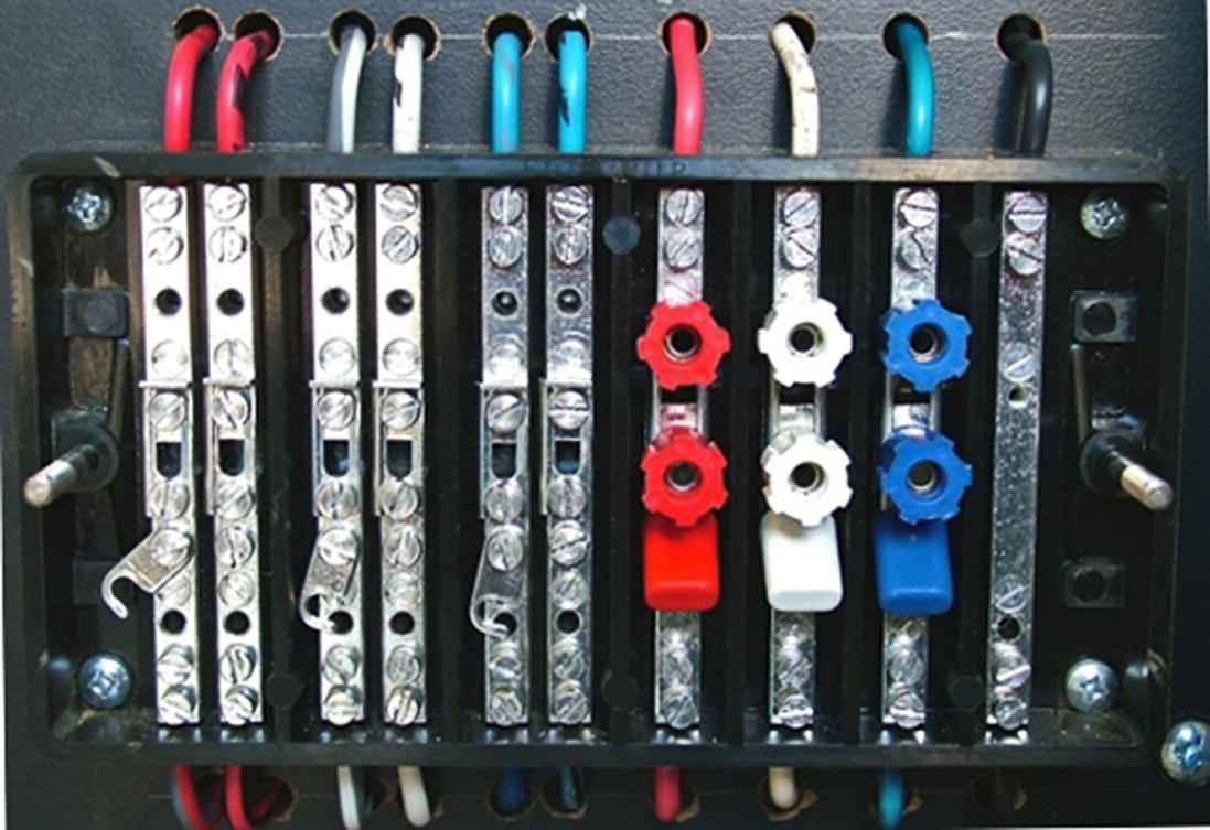
Figure 10.18 Typical metering test block, cover removed. (The CT links are on the left, and colour coded voltage terminals are on the right).
The test block facilitates both meter testing and auditing of the metering installation. It permits the measurement of CT secondary currents or the phase angle between a voltage and its respective current. This is achieved by inserting either an ammeter or a phase angle meter (PAM) into the CT circuit and then opening the CT links. (In the case of phase angle measurements, the PAM must also be provided with the element voltage, as well as its current, in order to display the phase angle between them.)
The test block is also useful when the meter is to be tested, whereupon the CT secondaries are shorted at the test block and isolated from the meter, using the links provided. Currents from a watt‐hour standard are injected into the meter. Most watt‐hour standards synchronise their test currents to the local three‐phase supply, which can be conveniently accessed from the potential terminals on the right‐hand side of the test block. By comparing the data in the meter with that calculated by the watt‐hour standard, the meter error can be evaluated.
10.8 Problems
- When the AC supply is taken at medium voltage potentials, the load is always metered on the MV side of the associated MV/LV distribution transformer(s), rather than on the LV side, where the bulk of the load is usually connected, as shown in Figure 10.19. The LV load often consists of a mixture of balanced three‐phase loads (such as induction motors) and single‐phase loads of various sizes. As a result there will usually be some neutral current flowing on the LV side, i.e. a zero‐sequence current exists there.

Figure 10.19 MV/LV distribution transformer.
The delta‐wye (Δ/Y) connected transformer supplying the load has a zero‐sequence current flowing within its delta winding, but not in the three‐wire circuit supplying it. We know that on the LV side, where the zero‐sequence current flows, the energy consumed can be correctly metered with a three‐element metering installation. However, since there is no zero‐sequence current present on the MV side, the question naturally arises, will a three‐element MV metering installation record the energy consumed correctly as well?
Consider an extreme case depicted in Figure 10.19, where a single‐phase resistive load is applied to the a phase on LV side of the transformer, while the b and c phases remain unloaded.
- Derive the associated line currents flowing on the MV side of the transformer, in terms of the current flowing in the A phase on the LV side. (For simplicity you may assume that this transformer has a 1:1 turns ratio, as shown in Figure 10.19, and assume also that the phase voltages are balanced.)
- Show that the energy recorded by a three‐element metering installation on the MV side equals that recorded by a similar installation on the LV side. You may assume that the transformer is lossless.
- Repeat part (b) for the case of a two‐element installation on the MV side.
- The results obtained in question 1 are really to be expected, otherwise MV metering would not be possible. We can demonstrate this for any unbalanced condition by considering the symmetrical components of the MV line currents and evaluating the power associated with each of them. We begin with a general expression for the three‐phase power flow (assuming balanced voltages), in terms of the sequence components of the current.

As we have seen, the three positive sequence currents in this expression sum to a total of 3VaI1 cos(ϕ1) watts.
- Expand the negative and zero‐sequence powers in the expression above and show that these sum to zero, provided the voltage contains positive sequence components only. Thus the total power measured is:

- Modify your answer to part (A) to allow for the general case where the phase voltages are also unbalanced. Show that the only terms in this expression that are non‐zero are those involving only positive sequence voltages and currents and negative sequence voltages and currents respectively, since in the case of a three‐wire load, zero‐sequence currents cannot exist, therefore:

- Expand the negative and zero‐sequence powers in the expression above and show that these sum to zero, provided the voltage contains positive sequence components only. Thus the total power measured is:
- An underground mining site, supplied by a 44 kV MV supply is metered with a two‐ element installation. After a meter test the A phase CT was accidentally left short‐circuited, meaning that the AB element was inoperative for a period of time. The meter did, however, continue to correctly record the CB element data, but it was only capable of recording the active and reactive energy imported from the bus throughout each 15 minute metering interval. The site consumes balanced currents and has power factor correction equipment installed and therefore its power factor tends to be quite high, typically lying between 0.92 and 0.95.
- Derive an expression for a correction factor k that can be applied to the measured data recorded for each metering interval, in order to obtain the correct energy consumed according to:
The correction factor k will be a function of the power factor of the load. In order to determine if k is a strong or a weak function of power factor, graph your expression for k over a range of power factors from 0.92 to 0.95. You should obtain a graph similar to that shown in Figure 10.20.

- If the median value of site power factor is chosen for the active energy correction, what is the maximum percentage error that can be expected in the corrected data?
- Can the active power maximum demand of the site be determined using this technique? If not, why not?
- Would k be as weak a function of power factor if the site’s power factor was uncorrected and was in the range 0.65–0.75? What error would you expect in this case?

Figure 10.20 Active energy correction factor, k as a function of load power factor.
- Derive an expression for a correction factor k that can be applied to the measured data recorded for each metering interval, in order to obtain the correct energy consumed according to:
-
- Derive an equivalent correction factor, K for the reactive energy recorded during each metering interval in question 3. Show by plotting a graph, that K is a strong function of the load power factor. Your graph should look like the one in Figure 10.21. Why is K negative in this particular case? Will it always be negative?
- Why can’t the reactive energy consumed by the site be recovered in the same way as the active? Explain.
- How might an estimate of the average reactive demand for the site be obtained assuming a median power factor? Explain.

Figure 10.21 Reactive energy correction factor, K as a function of load power factor. - Figure 10.22 shows a variation on the standard two‐element metering installation, which uses only one CT and two line connected VTs. This arrangement, known as negative B phase metering, is often used to provide a check metering installation using the B phase CT when the other two CTs are already used in a Blondel compliant two‐element arrangement.
- Sketch the phasor diagram for this installation, showing the relationship between the voltage and current as seen by each element. Assume that the phase currents lag their respective phase voltages by 10°.
- From your phasor diagram, determine the angle between the voltage and current as seen by each element, in terms of the load phase angles. In other words, derive expressions for ϕAB and ϕCB, the angles between the current and voltage applied to each meter element.
- Write an expression for the total power measured by the meter. Compare this with the expression for a standard two‐element installation. Under what conditions will the two expressions be equal? Is this circuit Blondel compliant? Why might it be used?

Figure 10.22 Negative B phase metering.
- The actual relationships between TCF, RCF and transformer phase errors γ and β appear below.

The linear Equations (10.27) and (10.28), provided in IEEE C57.13, are an approximation to these and make their interpretation simpler. If the ratio
 can be written in the form
  where
where  show that
  , and hence derive Equations (10.27) and (10.28), repeated here:

- The metering transformers on the site of a large HV connected industrial customer were upgraded and, at the customer’s request, the old metering installation was retained for some time so that performance of the old and new could be compared. Power data was averaged over many metering intervals to remove any timing jitter and then corrected for the known CT, VT and meter errors in each case. Using the data in Table 10.8, correct the measured power and show that, when corrected, both installations are effectively same.
Table 10.8 Comparative data of new and old metering. (You may assume that each set of current transformers share the same errors, as do each set of voltage transformers.)
VT magnitude error
(%)CT magnitude error
(%)VT phase error
(min)CT phase error
(min)Meter error
(%)Load power factor Average metered power (kW) New installation 0.436 −0.082 −6 5 0.02 0.95 126234 Old installation 0.156 −0.075 −2 4 −0.36 0.95 125391 Answer: Corrected power
(kW)New installation
125634Old installation
125670 - S vectors (VA vectors) – Equations 10.1 and 10.2 show that the active and reactive power measured by each metering element are related to the element volt‐amp product and the angle by which the phase current lags the phase voltage. This suggests that it might be useful to consider an S vector (or a VA vector) for each metering element, whose magnitude is equal to the volt‐amp product seen by that element, and whose angle is equal to that by which the element current lags the element voltage. These vectors can be plotted on the P‐Q plane, as depicted in Figure 10.23. S vectors are not phasors in that they do not represent sinusoidal quantities, but they do possess similar properties and can be manipulated in a similar fashion.

Figure 10.23 S vectors for a three‐element metering installation.
Figure 10.23 shows S vectors for a three‐element metering installation in which the meter sums the active and reactive energy contribution from each element. Figure 10.24 shows the S vectors for both three‐ and two‐element metering installations, in this case for a balanced load. Provided the phase currents sum to zero, the total active and reactive energy metered by each installation will be equal.

Figure 10.24 S vectors for three‐ and two‐element metering installations for a balanced load.
Consider the vector plot in Figure 10.25, where the load currents are unbalanced. Show that the only possible location for the b phase vector Sb (shown dotted) requires that
 . What implication can be drawn when
  ?
?
Figure 10.25 S vectors for three‐ and two‐element metering installations with an unbalanced load.
10.9 Sources
- 1 Independent Electricity Market Operator IMO market manual 3: metering Part 3.4; measurement error correction, IMO, USA.
- 2 United States Department of the Interior, Bureau of Reclamation, Watt‐hour meter maintenance and testing 2000, Facilities Engineering Branch, Colorado.
- 3 IEEE.C57.13, IEEE standard requirements for instrument transformers, 2008, IEEE Power Engineering Society, New York.
- 4 IEEE.C57.13.6, IEEE standard for high‐accuracy instrument transformers 2005, IEEE Power Engineering Society, New York.
- 5 IEC 60044.1, Instrument Transformers: Part 1 current transformers 2007, International Electrotechnical Commission, Geneva.
- 6 IEC 60044‐2, Instrument transformers: Part2 voltage transformers 2007, International Electrotechnical Commission, Geneva.
- 7 IEC 61869‐2, Instrument transformers – Part 2: additional requirements for current transformers 2012, International Electrotechnical Commission, Geneva.
- 8 IEC 61869‐3, Instrument transformers – Part 2: additional requirements for voltage transformers 2012, International Electrotechnical Commission, Geneva.
- 9 IEC 62053.22, Electricity metering equipment (AC) – Part 22 static meters for active energy (classes 0.2S and 0.5S), 2003, International Electrotechnical Commission, Geneva.
- 10 GE, Manual of instrument transformers, operation principles and application information General Electric.
- 11 ESAA, Manual of Australian metering practice, 1971, Electricity Supply Association of Australia, Melbourne.