
CHAPTER 7
Portfolio Optimization: Theory and Practice
Alumni Professor of Financial Modeling and
Stochastic Optimization (Emeritus),
University of British Columbia
Distinguished Visiting Research Associate
Systemic Risk Center, London School of Economics
STATIC PORTFOLIO THEORY
In the static portfolio theory case, suppose there are n assets, i = 1, …, n, with random returns ξ1, …, ξn. The return on asset i, namely ξi, is the capital appreciation plus dividends in the next investment period such as monthly, quarterly, or yearly or some other time period. The n assets have the distribution F(ξ1, …, ξn) with known mean vector ξ = (ξ1, …, ξn) and known n × n variance-covariance matrix Σ with typical covariance σij for i ≠ j and variance ![]() for i = j. A basic assumption (relaxed in section 6) is that the return distributions are independent of the asset weight choices, so F ≠ φ(x).
for i = j. A basic assumption (relaxed in section 6) is that the return distributions are independent of the asset weight choices, so F ≠ φ(x).
A mean-variance frontier is

where e is a vector of ones, x = (x1, …, xn) are the asset weights, K represents other constraints on the x, and w0 is the investor's initial wealth.
When variance is parameterized with δ > 0, it yields a concave curve, as in Figure 7.1(a). This is a Markowitz (1952, 1987, 2006) mean-variance efficient frontier and optimally trades off mean, which is desirable, with variance, which is undesirable. Tobin (1958) extended the Markowitz model to include a risk-free asset with mean ξ0 and no variance. Then the efficient frontier concave curve becomes the straight line as shown in Figure 7.1(b). The standard deviation here is plotted rather than the variance to make the line straight. An investor will pick an optimal portfolio in the Markowitz model by using a utility function that trades off mean for variance or, equivalently, standard deviation, as shown in Figure 7.1(a), to yield portfolio A. For the Tobin model, one does a simpler calculation to find the optimal portfolio that will be on the straight line in Figure 7.1(b) between the risk-free asset and the market index M. Here, the investor picks portfolio B that is two-thirds cash (risk-free asset) and one-third market index. The market index may be proxied by the S&P500 or Wilshire 5000 value weighted indices. Since all investors choose between cash and the market index, this separation of the investor's problem into finding the market index independent of the investor's assumed concave utility function and then where to be on the line for a given utility function is called Tobin's separation theorem. Ziemba, Parkan, and Brooks-Hill (1974) discuss this and show how to compute the market index and optimal weights of cash and the market index for various utility functions and constraints. They show how to calculate the straight-line efficient frontier in Figure 1 with a simple n variable deterministic linear complementary problem or a quadratic program. That calculation of Tobin's separation theorem means that for every concave, nondecreasing utility function u, the solution of the optimal ratio of risky assets, i = 1, …, n, is the same. Hence, ![]() is the same for all u ∊ U2 = [u|u′ ≥ 0, u″ ≤ 0].
is the same for all u ∊ U2 = [u|u′ ≥ 0, u″ ≤ 0].

FIGURE 7.1 Two efficient frontiers: (a) Markowitz mean-variance efficient frontier; (b) Tobin's risk-free asset and separation theorem.

where ![]() , ξ0 is the risk-free asset, and ξ ∼ N(ξ, Σ) with initial wealth w0 = 1.
, ξ0 is the risk-free asset, and ξ ∼ N(ξ, Σ) with initial wealth w0 = 1.
In step 1, one solves the n-variable deterministic linear complementary problem (LCP),
![]()
where ![]() m or the quadratic program min
m or the quadratic program min ![]() s.t. z ≥ 0 for the optimal risky asset weights, which are
s.t. z ≥ 0 for the optimal risky asset weights, which are
![]()
This LCP is derived as follows. The slope of the efficient frontier line in Figure 7.1 is found by

which is equivalent to

where ![]() .
.
Since g(x) is linear homogeneous and assuming λx ∈ K, where g(λx) = g(x) for λ ≥ 0, then the Kuhn–Tucker conditions can be written as the LCP problem above, where ![]() , and Σi is the ith row of Σ. From the theory of the LCP, see, for example, Murty (1972); there is a unique solution, since Σ is positive definite.
, and Σi is the ith row of Σ. From the theory of the LCP, see, for example, Murty (1972); there is a unique solution, since Σ is positive definite.
This gives the market index ![]() independent of u. Then in step 2, one determines the optimal ratio of M and the risk-free asset. So for a given u ∈ U2 from the single variable α ∈ (−∞, 1], in Figure 7.1(b), α = 1 is M, α = 1/2 if half M and half ξ0, and α = −3 means that three of the risk-free asset ξ0 is borrowed to invest four in M. The optimal allocation in the risk-free asset is α*, and the optimal allocation in risky asset i, i = 1, …, n is
independent of u. Then in step 2, one determines the optimal ratio of M and the risk-free asset. So for a given u ∈ U2 from the single variable α ∈ (−∞, 1], in Figure 7.1(b), α = 1 is M, α = 1/2 if half M and half ξ0, and α = −3 means that three of the risk-free asset ξ0 is borrowed to invest four in M. The optimal allocation in the risk-free asset is α*, and the optimal allocation in risky asset i, i = 1, …, n is ![]() , i = 1, …, n, which are obtained by solving
, i = 1, …, n, which are obtained by solving
where M = ξ′x* ∼ N(ξ′x*, x*′Σx*), and ξ = (ξ1, …, ξn).
One may solve (7.2) using a search algorithm such as golden sections or a bisecting search; see Zangwill (1969). Examples with data and specific utility functions appear in Ziemba, Parkan, and Brooks-Hill (1974). Ziemba (1974) generalized this to certain classes of infinite variance stable distributions. That analysis, though more complex, follows the normal distribution case. In place of variances, dispersions are used. Under the assumptions one has the convexity of the risk measure property that is analogous to Figure 7.1. That paper, as well as many other important classic papers, discussions, and extensive problems, are reprinted in Ziemba and Vickson (1975, 2006).
Figure 7.1(b) illustrates the Sharpe (1964)–Lintner (1965)–Mossin (1966) capital asset pricing model, which has E(Ri) = αi + βiE(RM), where E(Ri) and E(RM) are the mean return of the asset and the market, respectively, αi is the excess return from this asset, and βi is the asset's correlation with the market, M.
Referring to Figure 7.1(a), the point A is determined through a trade-off of expected return and variance. This trade-off is determined through risk aversion. The standard way to measure absolute risk aversion is via the Arrow (1965)–Pratt (1964) absolute risk aversion index
![]()
Risk tolerance as used in the investment world is

RA = 4, represents the standard pension fund strategy 60–40 stock bond mix corresponds to RT = 50 (independent of wealth).
RA(w) represents all the essential information about the investor's utility function u(w), which is only defined up to a linear transformation, while eliminating everything arbitrary about u, since
![]()
The major theoretical reasons for the use of RA is

where the risk premium π(w, z) is defined so that the decision maker is indifferent to receiving the random risk z and the nonrandom amount z − π = −π, where z = 0 and u[w − π] = Ezu(w + z) (this defines π). When u is concave, π ≥ 0.
For ![]() small, a Taylor series approximation yields
small, a Taylor series approximation yields
![]()
and for the special risk
where p(w, h) = probability premium = P(z = h) − P(z + h) such that the decision maker is indifferent between status quo and the risk z.

Equation 7.3 defines p.
By a Taylor series approximation, ![]() small errors.
small errors.
So risk premiums and probability premiums rise when risk aversion rises and vice versa.
Good utility functions, such as those in the general class of decreasing risk aversion functions u′(w) = (wa + b)−c, a > 0, c > 0, contain log, power, negative power, arctan, and so on. Decreasing absolute risk aversion utility functions are preferred because they are the class where a decision maker attaches a positive risk premium to any risk (π(w, z) > 0), but a smaller premium to any given risk the larger his wealth

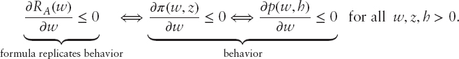
So decreasing absolute risk-aversion utility functions replicates those where the risk premium and probability premium are decreasing in wealth.
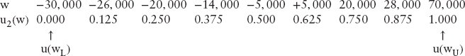
An individual's utility function and risk aversion index can be estimated using the double exponential utility function
![]()
where a, b, and c are constants. An example using the certainty-equivalent and gain-and-loss equivalent methods is in Figure 7.2 for Donald Hausch (my coauthor of various horse-racing books and articles) when he was a student. See the appendix, which describes these estimation methods. This function is strictly concave and strictly increasing and has decreasing absolute risk aversion.

Hausch's utility function was fit by least squares, and both methods provide similar curves. His absolute risk aversion is decreasing, see Figure 7.3(a,b), and nearly constant in his investment range where initial wealth w0 changes by ±10, 000 corresponding to RA between 2.0 and 2.5.

His relative risk aversion is increasing and linear in his investment range.
The Arrow–Pratt risk aversion index is the standard way to measure risk aversion, but the little-known Rubinstein risk aversion measure is actually optimal, assuming normal (discussed here) or symmetric distributions. Indeed, Kallberg and Ziemba (1983) showed that given utility functions u1 and u2, initial wealth w1 and w2, and assets (ξ1, …, ξn) ∼ N(ξ, Σ), and then if
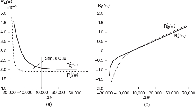
FIGURE 7.3 Risk aversion functions for Donald Hausch (a) absolute risk aversion function estimated by the certainly equivalent method (1) and gain and loss equivalent method; (b) relative risk aversion function estimated by the certainly equivalent method (1) and gain and loss equivalent method (2).
![]()
then x* solves
![]()
Hence, if two investors have the same Rubinstein risk aversion measure, they will then have the same optimal portfolio weights. As shown in Figure 7.4a,b,c,d, special exponential and negative power with the same average risk aversion have very similar mean, variance, expected utility, and portfolio weights and these are very different than with quadratic or exponential utility. When two utility functions have the same average risk aversion, then they have very similar optimal portfolio weights. Here u4(w) = e−β4/w and u6(w) = (w − w0)−β6 are different utility functions but their average risk aversions have similar ranges, and these are very different than the quadratic and exponential utilities in Figure 7.4a,b. The size of the errors is shown in Table 7.1 for fixed risk aversion of RA = 4.
The basic theory of Markowitz, Sharpe, and Tobin assumes that the parameters are known. The real world, of course, does not have constant parameters. So let's look first at the errors associated with parameter errors and later at models (stochastic programming) where the probability distribution of asset returns is explicitly considered.


FIGURE 7.4 Functional forms asset weights: (a) Quadratic monthly U1(w) = w − β1w2; (b) Exp monthly U2(w) = 1 − e−β2w; (c) Special exp monthly ![]() ; (d) Neg power monthly U6(w) = (w − W0)−β6.
; (d) Neg power monthly U6(w) = (w − W0)−β6.
Source: Kallberg and Ziemba, 1983
IMPORTANCE OF MEANS
Means are by far the most important part of any return distribution for actual portfolio results. If you are to have good results in any portfolio problem, you must have good mean estimates for future returns:
If asset X has cumulative distribution F(·) and asset Y has G(·) and these cumulative distribution functions cross only once, then asset X dominates asset Y for all increasing concave utility functions, that is, has higher expected utility, if and only if the mean of X exceeds the mean of Y.
This useful result of Hanoch and Levy (1969) implies that the variance and other moments are unimportant for single crossing distributions. Only the means count. With normal distributions, X and Y will cross only once if and only if the standard deviation of asset X is less than the standard deviation of asset Y. This is the basic equivalence of mean-variance analysis and expected utility analysis via second-order (concave, nondecreasing) stochastic dominance. This is shown in Figure 7.5, where the second-degree and mean-variance dominance is on the left. There is no dominance on the right because there are two crosses. This F has a higher mean but also higher variance than G. The densities f and g are plotted here for convenience and give the same results as if the cumulative distribution functions F and G were plotted.
Errors in inputs can lead to significant losses (Figure 7.6) and larger turnover (Figure 7.7). Additional calculations appear in Kallberg and Ziemba (1981, 1984) and Chopra and Ziemba (1993).
The error depends on the risk tolerance, the reciprocal of the Arrow–Pratt risk aversion  . However See Table 7.2, errors in means, variances, and covariances are roughly 20:2:1 times as important, respectively. But with low risk aversion, like log, the ratios can be 100:2:1. So good estimates are by far the most crucial aspect for successful application of a mean-variance analysis, and we will see that in all other stochastic modeling approaches.
The sensitivity of the mean carries into multiperiod models. There the effect is strongest in period 1, then less and less in future periods; see Geyer and Ziemba (2008). This is illustrated in Figures 7.8 and 7.9 for a five-period, 10-year model designed for the Siemen's Austria pension fund that is discussed later in this chapter. There it is seen that in period 1, with bond means for the U.S. and Europe in the 6 to 7 percent area, the optimal allocation to European and U.S. equity can be fully 100 percent.

FIGURE 7.5 Mean variance and second order stochastic dominance: (a) Dominance does not exist; (b) Dominance exists.

FIGURE 7.6 Mean percentage cash equivalent loss due to errors in inputs.
Source: Chopra-Ziemba, 1993

FIGURE 7.7 Average turnover for different percentage changes in means, variances, and covariances.
Source: Chopra, 1993


FIGURE 7.8 Optimal equity and bond allocations in period 1 of the InnoALM model.
Source: Geyer and Ziemba 2008

FIGURE 7.9 The effects of state-dependent correlations: optimal weights conditional on quintiles of portfolio weights in periods 2 and 5 of the InnoALM model: (a) Stage 2; (b) Stage 5.
Source: Geyer and Ziemba 2008
STOCHASTIC PROGRAMMING APPROACH TO ASSET LIABILITY MANAGEMENT
I now discuss my approach using scenarios and optimization to model asset-liability decisions for pension funds, insurance companies, individuals, retirement, bank trading departments, hedge funds, and so on. It includes the essential problem elements: uncertainties, constraints, risks, transactions costs, liquidity, and preferences over time, to provide good results in normal times and avoid or limit disaster when extreme scenarios occur. The stochastic programming approach, while complex, is a practical way to include key problem elements that other approaches are not able to model.
Other approaches (static mean variance, fixed mix, stochastic control, capital growth, continuous time finance, etc.) are useful for the microanalysis of decisions, and the SP approach is useful for the aggregated macro (overall) analysis of relevant decisions and activities. They yield good results most of the time, but frequently lead to the recipe for disaster: overbetting and not being truly diversified at a time when an extreme scenario occurs. It pays to make a complex stochastic programming model when a lot is at stake and the essential problem has many complications.
The accuracy of the actual scenarios chosen and their probabilities contribute greatly to model success. However, the scenario approach generally leads to superior investment performance, even if there are errors in the estimations of both the actual scenario outcomes and their probabilities. It is not possible to include all scenarios, or even some that may actually occur. The modeling effort attempts to cover well the range of possible future evolution of the economic environment. The predominant view is that such models do not exist, are impossible to successfully implement, or are prohibitively expensive. I argue that given modern computer power, better large-scale stochastic linear programming codes, and better modeling skills, such models can be widely used in many applications and are very cost effective.
We know from Harry Markowitz's work and that of others that mean-variance models are useful in an assets-only situation. From my consulting at Frank Russell, I know that professionals adjust means (mean-reversion, James-Stein, etc.) and constrain output weights.
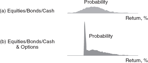
They do not change asset positions unless the advantage of the change is significant. Also, they do not use mean-variance analysis with liabilities and other major market imperfections except as a first test analysis. Mean-variance models can be modified and applied in various ways to analyze many problems; see Markowitz (1987) and Grinold and Khan (1999) for examples. Masters of this have used Barra Risk Factor Analysis, which analyzes any question via a simple mean-variance model. But mean-variance models define risk as a terminal wealth surprise, regardless of direction, and make no allowance for skewness preference. Moreover, they treat assets with option features inappropriately, as shown in Figure 7.10.
But we will use in my models a relative of variance—namely, the convex risk measure weighted downside target violations—and that will avoid such objections.

Asset-liability problems can be for institutions or individuals (Figure 7.11). My experience is that the latter is much more difficult because one must make models useful for many individuals, and people change their assets, goals, and preferences, and hide assets. Basic references are Ziemba and Mulvey (1998), Zenios and Ziemba (2006, 2007), and Gassman and Ziemba (2013) that contain theory, computations, and many case studies. See also Wallace and Ziemba (2005), which has descriptions of computer codes as well as applications.
Possible approaches to model ALM situations include:
- Simulation: There is usually too much output to understand, but it is very useful as check.
- Mean variance: This is okay for one period but hard to use in multiperiod problems and with liabilities. It assumes means and variances are known.
- Expected log: Very risky strategies that do not diversify well; fractional Kelly with downside constraints are excellent for multiperiod risky investment betting (see Section 6).
- Stochastic control: Bang-bang policies; see the Brennan-Schwartz paper in Ziemba and Mulvey (1998) on how to constrain to be practical.
- Stochastic programming/stochastic control: Mulvey—see Mulvey (1996), Mulvey and Pauling (2002), and Mulvey et al. (2007)—uses this approach, which is a form of volatility pumping, discussed in general by Luenberger (1998).
- Stochastic programming: This is my approach.
Continuous time modeling, though popular in the academic world, seems to be impractical in the real world, as Figure 7.12 shows. Here, the asset proportions from a Merton (1992) stochastic control type model are stocks, bonds, and interest rate futures representing spot and future interest rates.
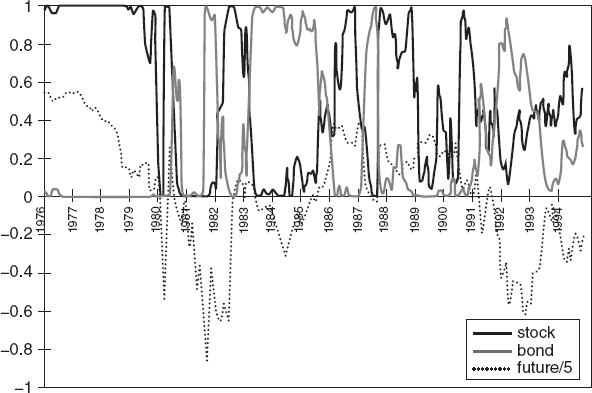
FIGURE 7.12 Asset weights over time with a stochastic control continuous time Merton type model.
Source: Brennan and Schwartz (1998)
The stochastic programming approach is ideally suited to analyze such problems with the following features:
- Multiple time periods; end effects—steady state after decision horizon adds one more decision period to the model
- Consistency with economic and financial theory for interest rates, bond prices, etc.
- Discrete scenarios for random elements—returns, liability costs, currency movements
- Utilization of various forecasting models, handle fat tails
- Institutional, legal, and policy constraints
- Model derivatives, illiquid assets, and transactions costs
- Expressions of risk in terms understandable to decision makers (the more you lose, the more is the penalty for losing)
- Maximize long-run expected profits net of expected discounted convex penalty costs for shortfalls, paying more and more penalty for shortfalls as they increase
- Model as constraints or penalty costs in the objective to maintain adequate reserves and cash levels and meet regularity requirements
We can now solve very realistic multiperiod problems on PCs. If the current situation has never occurred before, then use one that's similar to add scenarios. For a crisis in Brazil, use Russian crisis data, for example. The results of the SP will give you good advice when times are normal and keep you out of severe trouble when times are bad.
Those using SP models may lose 5, 10, or even 15 percent, but they will not lose 50, 70, or even 95 percent, like some investors and hedge funds. If the scenarios are more or less accurate and the problem elements reasonably modeled, the SP will give good advice. You might slightly underperform in normal markets but you will greatly overperform in bad markets when other approaches may blow up.
These models make you diversify, which is the key for keeping out of trouble. My work in stochastic programming began in my Ph.D. work at Berkeley. In 1974, I taught my first stochastic programming class and that led to early papers with my students Jarl Kallberg and Martin Kusy; see Kallberg, White and Ziemba (1982) and Kusy and Ziemba (1986). Table 7.3 illustrates the models we built at Frank Russell in the 1990s.
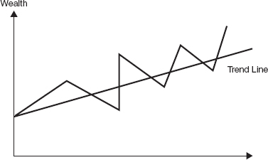
In Cariño, Myers, and Ziemba (1998), we showed that stochastic programming models usually beat fix-mix models. The latter are basically volatility pumping models (buy low, sell high); see Luenberger (1998). Figure 7.13 illustrates how the optimal weights change, depending on previous periods’ results. Despite good results, fixed-mix and buy-and-hold strategies do not utilize new information from return occurrences in their construction. By making the strategy scenario dependent using a multiperiod stochastic programming model, a better outcome is possible.


FIGURE 7.13 Example portfolios: (a) Initial portfolios of the three strategies; (b) Contingent allocations at year one.
- The dynamic stochastic programming strategy, which is the full optimization of the multiperiod model; and
- The fixed mix in which the portfolios from the mean-variance frontier have allocations rebalanced back to that mix at each stage; buy when low and sell when high. This is like covered calls, which is the opposite of portfolio insurance.
Consider fixed mix strategies A (64–36 stock–bond mix) and B (46–54 stock–bond mix). The optimal stochastic programming strategy dominates as shown in Figure 7.14.
A further study of the performance of stochastic dynamic and fixed-mix portfolio models was made by Fleten, Høyland, and Wallace (2002). They compared two alternative versions of a portfolio model for the Norwegian life insurance company Gjensidige NOR, namely multistage stochastic linear programming and the fixed-mix constant rebalancing study. They found that the multiperiod stochastic programming model dominated the fixed-mix approach but the degree of dominance is much smaller out-of-sample than in-sample; see Figure 7.15. This is because out-of-sample, the random input data are structurally different from in-sample, so the stochastic programming model loses its advantage in optimally adapting to the information available in the scenario tree. Also, the performance of the fixed-mix approach improves because the asset mix is updated at each stage.


FIGURE 7.15 Comparison of advantage of stochastic programming over fixed mix model in and out of sample: (a) In-sample; (b) Out-of-sample.
Source: Fleten et al. (2002)
The Russell-Yasuda Kasai was the first large-scale multiperiod stochastic programming model implemented for a major financial institution; see Henriques (1991). As a consultant to the Frank Russell Company during 1989 to 1991, I designed the model. The team of David Cariño, Taka Eguchi, David Myers, Celine Stacy, and Mike Sylvanus at Russell in Tacoma, Washington, implemented the model for the Yasuda Fire and Marine Insurance Co., Ltd. in Tokyo under the direction of research head Andy Turner. Roger Wets and my former UBC Ph.D. student Chanaka Edirishinghe helped as consultants in Tacoma, and Kats Sawaki was a consultant to Yasuda Kasai in Japan to advise them on our work. Kats, a member of my 1974 UBC class in stochastic programming where we started to work on ALM models, was then a professor at Nanzan University in Nagoya and acted independently of our Tacoma group. Kouji Watanabe headed the group in Tokyo, which included Y. Tayama, Y. Yazawa, Y. Ohtani, T. Amaki, I. Harada, M. Harima, T. Morozumi, and N. Ueda.
Experience has shown that we should not be concerned with getting all the scenarios exactly right when using stochastic programming models. You cannot do this, and it does not matter much, anyway. Rather, you should worry that you have the problem periods laid out reasonably and that the scenarios basically cover the means, the tails, and the chance of what could happen.
Back in 1990/1991, computations were amajor focus of concern. I knew how to formulate the model, which was an outgrowth of Kallberg, White, and Ziemba (1982) and Kusy and Ziemba (1986). David Cariño did much of the formulation details. Originally, we had 10 periods and 2,048 scenarios. It was too big to solve at that time and became an intellectual challenge for the stochastic programming community. Bob Entriken, D. Jensen, R. Clark, and Alan King of IBM Research worked on its solution but never quite cracked it. We quickly realized that 10 periods made the model far too difficult to solve and also too cumbersome to collect the data and interpret the results, and the 2,048 scenarios were at that time too large a number to deal with. About two years later, Hercules Vladimirou, working with Alan King at IBM Research, was able to effectively solve the original model using parallel processing on several workstations.
The Russell-Yasuda model was designed to satisfy the following need as articulated by Kunihiko Sasamoto, director and deputy president of Yasuda Kasai:
The liability structure of the property and casualty insurance business has become very complex, and the insurance industry has various restrictions in terms of asset management. We concluded that existing models, such as Markowitz mean variance, would not function well and that we needed to develop a new asset/liability management model.
The Russell-Yasuda Kasai model is now at the core of all asset/liability work for the firm. We can define our risks in concrete terms, rather than through an abstract measure like, in business terms, standard deviation. The model has provided an important side benefit by pushing the technology and efficiency of other models in Yasuda forward to complement it. The model has assisted Yasuda in determining when and how human judgment is best used in the asset/liability process (Cariño et al., 1994). The model was a big success and of great interest both in the academic and institutional investment asset-liability communities.
The Yasuda Fire and Marine Insurance Company
The Yasuda Fire and Marine Insurance Company called Yasuda Kasai (meaning fire) is based in Tokyo. It began operations in 1888 and was the second largest Japanese property and casualty insurer and seventh largest in the world by revenue in 1989. Its main business was voluntary automobile (43.0 percent), personal accident (14.4 percent), compulsory automobile (13.7 percent), fire and allied (14.4 percent), and other (14.5 percent). The firm had assets of 3.47 trillion yen (US$26.2 billion) at the end of fiscal 1991 (March 31, 1992). In 1988, Yasuda Kasai and Russell signed an agreement to deliver a dynamic stochastic asset allocation model by April 1, 1991. Work began in September 1989. The goal was to implement a model of Yasuda Kasai's financial planning process to improve its investment and liability payment decisions and overall risk management. In 1989, after Russell could not determine how to do this, I proposed a stochastic programming model, which we then built at Russell in Tacoma.
The business goals were to:
- Maximize long run expected wealth.
- Pay enough on the insurance policies to be competitive in current yield.
- Maintain adequate current and future reserves and cash levels.
- Meet regulatory requirements, especially with the increasing number of saving-oriented policies being sold that were generating new types of liabilities.
The following is a summary of the Russell Yasuda model and its results. See, also, the original papers by Cariño Ziemba et al. (1994, 1998ab) and the survey by Ziemba (2006):
- The model needed to have more realistic definitions of operational risks and business constraints than the return variance used in previous mean-variance models used at Yasuda Kasai.
- The implemented model determines an optimal multiperiod investment strategy that enables decision makers to define risks in tangible operational terms such as cash shortfalls.
- The risk measure used is convex and penalizes target violations more and more as the violations of various kinds and in various periods increase.
- The objective is to maximize the discounted expected wealth at the horizon net of expected discounted penalty costs incurred during the five periods of the model.
- This objective is similar to a mean-variance model, except that it is over five periods and only counts downside risk through target violations.
- I greatly prefer this approach to VaR or CVaR and its variants for ALM applications because for most people and organizations, the nonattainment of goals is more and more damaging, not linear in the nonattainment (as in CVaR) or not considering the size of the nonattainment at all (as in VaR); see Ziemba (2013).
- A reference on VaR and CVaR as risk measures is Artzner et al. (1999). They argue that good risk measures should be coherent and satisfy a set of axioms.
The convex risk measure I use is coherent. Rockafellar and Ziemba (2013) define a set of axioms that justify these convex risk measures:
- The model formulates and meets the complex set of regulations imposed by Japanese insurance laws and practices.
- The most important of the intermediate horizon commitments is the need to produce income sufficiently high to pay the required annual interest in the savings type insurance policies without sacrificing the goal of maximizing long-run expected wealth.
- During the first two years of use, fiscal 1991 and 1992, the investment strategy recommended by the model yielded a superior income return of 42 basis points (US$79 million) over what a mean-variance model would have produced. Simulation tests also show the superiority of the stochastic programming scenario–based model over a mean-variance approach.
- In addition to the revenue gains, there have been considerable organizational and informational benefits.
- The model had 256 scenarios over four periods, plus a fifth end-effects period.
- The model is flexible regarding the time horizon and length of decision periods, which are multiples of quarters.
- A typical application has initialization, plus period 1 to the end of the first quarter; period 2 the remainder of fiscal year 1; period 3 the entire fiscal year 2, period 4 fiscal years 3, 4, and 5; and period 5, the end effects years 6 on to forever.
Figure 7.16 shows the multistage stochastic linear programming structure of the Russell-Yasuda Kasai model.
The basic formulation of the model is as follows. The objective of the model is to allocate discounted fund value among asset classes to maximize the expected wealth at the end of the planning horizon T less expected penalized shortfalls accumulated throughout the planning horizon:

subject to budget constraints
![]()
asset accumulation relations
![]()
income shortfall constraints
![]()

and non-negativity constraints
![]()
for t = 0, 1, 2, …, T − 1. Liability balances and cash flows are computed to satisfy the liability accumulation relations
![]()
Publicly available codes to solve such models are discussed in Wallace and Ziemba (2005); see also Gonzio and Kouwenberg (2001). The Russell–Yasuda model is small by 2015 standards, but in 1991, it was a challenge. The dimensions of a typical implemented problem are shown in Table 7.4.
Figure 7.17 shows Yasuda Kasai's asset liability decision making process.
Yasuda Fire and Marine faced the following situation:
- An increasing number of savings-oriented policies were being sold, which had new types of liabilities.
- The Japanese Ministry of Finance imposed many restrictions through insurance law that led to complex constraints.
- The firm's goals included both current yield and long-run total return, and that led to multidimensional risks and objectives.
The insurance policies were complex, with a part being actual insurance and another part an investment with a fixed guaranteed amount, plus a bonus dependent on general business conditions in the industry. The insurance contracts are of varying length—maturing, being renewed or starting in various time periods—and subject to random returns on assets managed, insurance claims paid, and bonus payments made. There are many regulations on assets, including restrictions on equity, loans, real estate, foreign investment by account, foreign subsidiaries, and tokkin (pooled accounts). The asset classes were:


| Asset | Associated Index |
| Cash bonds | Nomura bond performance index |
| Convertible bonds | Nikko research convertible bond index |
| Domestic equities | TOPIX |
| Hedged foreign bonds | Salomon Brothers world bond index (or hedged equivalent) |
| Hedged foreign equities | Morgan Stanley world equity index (or hedged equivalent) |
| Unhedged foreign bonds | Salomon Brothers world bond index |
| Unhedged foreign equities | Morgan Stanley world equity index |
| Loans | Average lending rates (trust/long-term credit (or long-term prime rates) |
| Money trusts, etc. | Call rates (overnight with collateral) |
| Life insurance company general accounts | |
To divide the universe of available investments into a manageable number of asset classes involves a trade-off between detail and complexity. A large number of asset classes would increase detail at the cost of increasing size. Therefore, the model allows the number and definition of asset classes to be specified by the user. There can be different asset classes in different periods. For example, asset classes in earlier periods can be collapsed into aggregate classes in later periods.
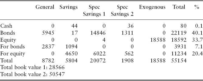
A major part of the information from the model is in the terms of reports consisting of tables and figures of model output. Actual asset allocation results from the model are confidential. But we have the following expected allocations in the initialization (Table 7.5) and end effects periods (Table 7.6). These are averages across scenarios in 100 million yen units and percentages by account.
TABLE 7.5 Expected Allocations for Initialization Period: INI (100 million yen: percentages by account).

- The 1991, Russell Yasuda Kasai Model was then the largest known application of stochastic programming in financial services.
- There was a significant ongoing contribution to Yasuda Kasai's financial performance—US$79 million and US$9 million in income and total return, respectively, over FY1991–1992—and it has been in use since then.
- The basic structure is portable to other applications because of flexible model generation. Indeed, the other models in Table 7.3 are modified versions of the Russell-Yasuda Kasai model.
- There is substantial potential impact in performance of financial services companies.
- The top 200 insurers worldwide have in excess of $10 trillion in assets.
- Worldwide pension assets are also about $7.5 trillion, with a $2.5 trillion deficit.
- The industry is also moving toward more complex products and liabilities and risk-based capital requirements.
SIEMENS INNOALM PENSION FUND MODEL
I made this model with Alois Geyer in 2000 for the Siemens Austria pension fund. The model has been in constant use since then and is described in Geyer and Ziemba (2008). I begin by discussing the pension situation in Europe.
There is rapid aging of the developed world's populations—the retiree group, those 65 and older, will roughly double from about 20 percent to about 40 percent of the worker group, those 15–64:
- Better living conditions, more effective medical systems, a decline in fertility rates, and low immigration into the Western world contribute to this aging phenomenon.
- By 2030, two workers will have to support each pensioner, compared with four now.
- Contribution rates will rise.
- Rules to make pensions less desirable will be made. For example, the United Kingdom, France, Italy, and Greece have raised or are considering raising the retirement age.
- Many pension funds worldwide are greatly underfunded.
Historically, stocks have greatly outperformed bonds and other assets; see Figure 7.18 which shows the relative returns in nominal terms. Long horizons have produced very high returns from stocks. However, the wealth ride is very rocky and in short periods, the stock market is risky. There can be long periods of underperformance. There have been four periods where equities have had essentially zero gains in nominal terms (not counting dividends): 1899 to 1919, 1929 to 1954, 1964 to 1981, and 2000 to 2009. Seen another way, since 1900, there have only been four periods with nominal gains: 1919 to 1929, 1954 to 1964, 1981 to 2000, and March 2009 to February 2015. Figure 7.19 shows the Dow Jones 30 stock price weighted index, real and nominal, from 1802 to 2006. This index does not include dividends, so it is very bumpy.

FIGURE 7.18 Emerging and developed market returns, 1900–2013
(Source: Credit Suisse Global Investment Returns Yearbook 2014)

FIGURE 7.19 Real equity returns and per capita GDP, 1900–2013
(Source: Credit Suisse Global Investment Returns Yearbook 2014)
Among other things, European pension funds, including those in Austria, have greatly underperformed those in the United States and the United Kingdom and Ireland largely because they greatly underweight equity. For example, Table 7.7 shows with the asset structure of European pension funds with Austria at 4.1 percent.
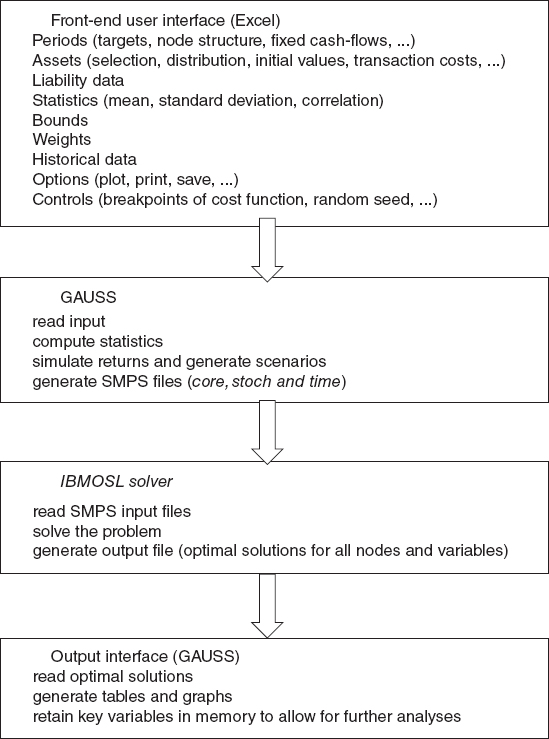
InnoALM is a multi-period stochastic linear programming model designed by Ziemba and implemented by Geyer with input from Herold and Kontriner for Innovest to use for Austrian pension funds (Figure 7.20). It is a tool to analyze Tier 2 pension fund investment decisions. It was developed in response to the growing worldwide challenges of aging populations and increased number of pensioners who put pressure on government services such as health care and Tier 1 national pensions to keep Innovest competitive in their high level fund management activities.

Siemens AG Österreich is the largest privately owned industrial company in Austria. Turnover (EUR 2.4 Bn. in 1999) is generated in a wide range of business lines including information and communication networks, information and communication products, business services, energy and traveling technology, and medical equipment.
- The Siemens Pension fund, established in 1998, is the largest corporate pension plan in Austria and follows the defined contribution principle.
- More than 15,000 employees and 5,000 pensioners are members of the pension plan with about EUR 500 million in assets under management.
- Innovest Finanzdienstleistungs AG, which was founded in 1998, acts as the investment manager for the Siemens AG Österreich, the Siemens Pension Plan, as well as for other institutional investors in Austria.
- With EUR 2.2 billion in assets under management, Innovest focuses on asset management for institutional money and pension funds.
- The fund was rated the first of 19 pension funds in Austria for the two-year 1999/2000 period.
Features of InnoALM.
- A multiperiod stochastic linear programming framework with a flexible number of time periods of varying length.
- Generation and aggregation of multiperiod discrete probability scenarios for random return and other parameters.
- Various forecasting models.
- Scenario dependent correlations across asset classes.
- Multiple covariance matrices corresponding to differing market conditions.
- Constraints reflect Austrian pension law and policy.
As in the Russell-Yasuda Kasai models, the objective function is a
- Concave risk-averse preference function that maximizes the expected present value of terminal wealth net of expected convex (piecewise linear) penalty costs for wealth and benchmark targets in each decision period.
- InnoALM user interface allows for visualization of key model outputs, the effect of input changes, growing pension benefits from increased deterministic wealth target violations, stochastic benchmark targets, security reserves, policy changes, and so on.
- The solution process using the IBMOSL stochastic programming code is fast enough to generate virtually online decisions and results and allows for easy interaction of the user with the model to improve pension fund performance.
The model has deterministic wealth targets that grow 7.5 percent per year; in a typical application the model also has stochastic benchmark targets on asset returns:
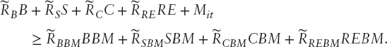
Bonds, stocks, cash, and real estate have stochastic benchmark returns with asset weights B, S, C, RE, M, with the shortfall to be penalized.
Examples of national investment restrictions on pension plans are as follows.
| Country | Investment Restrictions |
| Germany | Max. 30% equities, max. 5% foreign bonds |
| Austria | Max. 40% equities, max. 45% foreign securities, min. 40% EURO bonds |
| France | Min. 50% EURO bonds |
| Portugal | Max. 35% equities |
| Sweden | Max. 25% equities |
| UK, U.S. | Prudent man rule |
The model gives insight into the wisdom of such rules, and portfolios can be structured around the risks:
- An Excel™ spreadsheet is the user interface.
- The spreadsheet is used to select assets, define the number of periods, and choose the scenario node-structure.
- The user specifies the wealth targets, cash inflows and outflows, and the asset weights that define the benchmark portfolio (if any).
- The input-file contains a sheet with historical data and sheets to specify expected returns, standard deviations, correlation matrices, and steering parameters.
- A typical application with 10,000 scenarios takes about 7 to 8 minutes for simulation, generating SMPS files and solving and producing output on a 1.2 Ghz Pentium III notebook with 376 MB RAM. For some problems, execution times can be 15 to 20 minutes.
When there is trouble in the stock market, the positive correlation between stocks and bonds fails and they become negatively correlated (Figures 7.21, 7.22). When the mean of the stock market is negative, bonds are most attractive, as is cash (See Table 7.8).
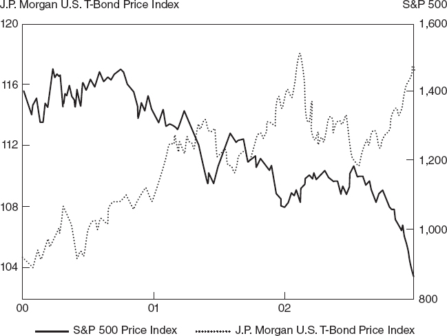
FIGURE 7.21 S&P500 index and U.S. government bond returns, 2000–2002.
Source: Schroder Investment Management Ltd. 2002


FIGURE 7.22 Rolling correlations between U.S. equity and government bond returns.
Source: Schroder Investment Management Ltd. 2002
Assumptions about the statistical properties of returns measured in nominal euros are based on a sample of monthly data from January 1970 for stocks and 1986 for bonds to September 2000. Summary statistics for monthly and annual log returns are in Table 7.9. The U.S. and European equity means for the longer period 1970–2000 are much lower than for 1986–2000 and slightly less volatile. The monthly stock returns are non-normal and negatively skewed. Monthly stock returns are fat tailed, whereas monthly bond returns are close to normal (the critical value of the Jarque-Bera test for a = .01 is 9.2).
We calculate optimal portfolios for seven cases: cases with and without mixing of correlations and consider normal, t-, and historical distributions. Cases NM, HM, and TM use mixing correlations. Case NM assumes normal distributions for all assets. Case HM uses the historical distributions of each asset. Case TM assumes t-distributions with five degrees of freedom for stock returns, whereas bond returns are assumed to have normal distributions. Cases NA, HA, and TA are based on the same distribution assumptions with no mixing of correlations matrices. Instead the correlations and standard deviations used in these cases correspond to an average period where 10 percent, 20 percent, and 70 percent weights are used to compute averages of correlations and standard deviations used in the three different regimes.
Comparisons of the average (A) cases and mixing (M) cases are mainly intended to investigate the effect of mixing correlations. Finally, in the case, TMC, we maintain all assumptions of case TM but use Austria's constraints on asset weights. Eurobonds must be at least 40 percent and equity at most 40 percent, and these constraints are binding.

A distinct pattern emerges:
- The mixing correlation cases initially assign a much lower weight to European bonds than the average period cases.
- Single-period, mean-variance optimization, and the average period cases (NA, HA, and TA) suggest an approximate 45–55 mix between equities and bonds.
- The mixing correlation cases (NM, HM, and TM) imply a 65–35 mix. Investing in U.S. bonds is not optimal at stage 1 in any of the cases, which seems due to the relatively high volatility of US bonds.
Optimal initial asset weights at Stage 1 by case are shown in Table 7.10.
If the level of portfolio wealth exceeds the target, the surplus is allocated to a reserve account and a portion used to increase (10 percent usually) wealth targets.
Table 7.11 has the expected terminal wealth levels, expected reserves, and probabilities of shortfall. TMC has the poorest results showing that the arbitrary constraints hurt performance. The mixing strategies NM, HM, and, especially, TM have the best results with the highest expected terminal wealthy, expected reserves and the lowest shortfall probabilities.

TABLE 7.11 Expected Terminal Wealth, Expected Reserves, and Probabilities of Shortfalls with a Target Wealth, Wt = 206.1.

In summary: optimal allocations, expected wealth, and shortfall probabilities are mainly affected by considering mixing correlations while the type of distribution chosen has a smaller impact. This distinction is mainly due to the higher proportion allocated to equities if different market conditions are taken into account by mixing correlations.
Geyer and I ran an out-of-sample test to see if the scenario-dependent correlation matrix idea adds value (Figure 7.23). It was assumed that in the first month wealth is allocated according to the optimal solution for stage 1. In subsequent months, the portfolio is rebalanced as follows:
- Identify the current volatility regime (extreme, highly volatile, or normal) based on the observed U.S. stock return volatility. It is assumed that the driving variable is U.S. volatility.
- Search the scenario tree to find a node that corresponds to the current volatility regime and has the same or a similar level of wealth.
- The optimal weights from that node determine the rebalancing decision.
- For the no-mixing cases NA, TA, and HA, the information about the current volatility regime cannot be used to identify optimal weights. In those cases, we use the weights from a node with a level of wealth as close as possible to the current level of wealth.

The following quote by Konrad Kontriner (member of the board) and Wolfgang Herold (senior risk strategist) of Innovest emphasizes the practical importance of InnoALM:
The InnoALM model has been in use by Innovest, an Austrian Siemens subsidiary, since its first draft versions in 2000. Meanwhile it has become the only consistently implemented and fully integrated proprietary tool for assessing pension allocation issues within Siemens AG worldwide. Apart from this, consulting projects for various European corporations and pensions funds outside of Siemens have been performed on the basis of the concepts of InnoALM.
The key elements that make InnoALM superior to other consulting models are the flexibility to adopt individual constraints and target functions in combination with the broad and deep array of results, which allows to investigate individual, path dependent behavior of assets and liabilities as well as scenario-based and Monte-Carlo-like risk assessment of both sides.
In light of recent changes in Austrian pension regulation the latter even gained additional importance, as the rather rigid asset-based limits were relaxed for institutions that could prove sufficient risk management expertise for both assets and liabilities of the plan. Thus, the implementation of a scenario-based asset allocation model will lead to more flexible allocation restraints that will allow for more risk tolerance and will ultimately result in better long-term investment performance.
Furthermore, some results of the model have been used by the Austrian regulatory authorities to assess the potential risk stemming from less constrained pension plans.
DYNAMIC PORTFOLIO THEORY AND PRACTICE: THE KELLY CAPITAL GROWTH APPROACH
The first category of multiperiod models are those reducable to static models. Part IV of Ziemba and Vickson (1975; 2006) reprints key papers and discusses important results of such models.
It is well known in stochastic programming that n-period concave stochastic programs are theoretically equivalent to concave static problems; see Dantzig (1955). In the theory of optimal investment over time, it is not quadratic (the utility function behind the Sharpe ratio) but log that yields the most long-term growth. But the elegant results on the Kelly (1956) criterion, as it is known in the gambling literature, and the capital growth theory, as it is known in the investments literature, are long-run asymptotic results; see the surveys by Hakansson and Ziemba (1995) and MacLean and Ziemba (2006) and Thorp (2006) that were proved rigorously by Breiman (1961) and generalized by Algoet and Cover (1988).
However, the Arrow–Pratt absolute risk aversion of the log utility criterion, namely 1/ω, is essentially zero. Hence, in the short run, log can be an exceedingly risky utility function with wide swings in wealth values (Figure 7.24). And fractional, Kelly strategies are not much safer as their risk aversion indices are 1/γω where the negative power utility function αWα, α < 0. This formula
![]()
is exact for lognormal assets and approximately correct otherwise; see MacLean, Ziemba, and Li (2005).
The myopic property of log utility (optimality is secured with today's data and you do not need to consider the past or future) is derived as follows in the simplest Bernoulli trials (p = probability you win, q = 1 − p = probability you lose a fixed amount).
Final wealth after N trials is
![]()
where f = fraction bet, X0 = initial wealth and you win M of N trials.
The exponential rate of growth is

Thus, the criterion of maximizing the long-run exponential rate of asset growth is equivalent to maximizing the one period expected logarithm of wealth. So an optimal policy is myopic. See Hakansson (1972) for generalizations of this myopic policy.
![]()
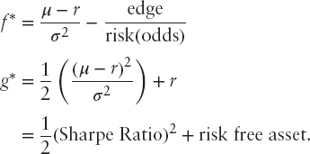
The optimal fraction to bet is the edge p − q. The bets can be large: ![]()

The key to the size of the bet is not the edge, it is the risk.
An example was the bet to place and show on Slew O'Gold in the inaugural Breeders’ Cup Classic in 1984: f* = 64 percent for place/show suggests fractional Kelly (that is, a lower bet where you blend the Kelly full expected log bet with cash). See the discussion of the Thorp-Ziemba bets on that day in Ziemba and Hausch (1986) and an expanded version in Ziemba (2015).
In continuous time,
The classic Breiman (1960; 1961) results are: in each period t = 1,2,… there are K investment opportunities with returns per unit invested XN1, …, XNk, intertemporally independent with finitely many distinct values.

Property 1: Maximizing E log XN asymptotically maximizes the rate of asset growth.
If in each time period, two portfolio managers have the same family of investment opportunities and one uses a Λ* maximizing
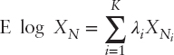
whereas the other uses an essentially different strategy; for example:
![]()
then

as essentially different means they differ infinitely often. So the actual amount of the fortune exceeds that with any other strategy by more and more as the horizon becomes more distant.
Property 2: The expected time to reach a preassigned goal is, asymptotically as X increases, least with a strategy maximizing E log XN.
We learn a lot from the following Kelly and half Kelly medium time simulations from Ziemba and Hausch (1986). This simulation had 700 independent investments, all with a 14 percent advantage, with 1,000 simulated runs and w0 = $1,000.
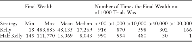
The power of the Kelly criterion is shown when 16.6 percent of the time final wealth is 100 times the initial wealth with full Kelly but only once with half Kelly. Thirty percent of the time, final wealth exceeds 50 times initial wealth. But the probability of being ahead is higher with half Kelly 87 percent versus 95.4 percent. So Kelly is much riskier than half Kelly. However, the minimum wealth is 18, and it is only 145 with half Kelly. So with 700 bets all independent with a 14 percent edge, the result is that you can still lose over 98 percent of your fortune with bad scenarios, and half Kelly is not much better with a minimum of 145 or a 85.5 percent loss. Here, financial engineering is important to avoid such bad outcomes.
Figures 7.25(a), (b) from MacLean, Thorp, Zhao, and Ziemba (2012) show the highest and lowest final wealth trajectories for full, ¾, ½, ¼, and ⅛ Kelly strategies for this example. Most of the gain is in the final 100 of the 700 decision points. Even with these maximum graphs, there is much volatility in the final wealth with the amount of volatility generally higher with higher Kelly fractions. Indeed with ¾ Kelly, there were losses from about decision points 610 to 670.
The final wealth levels are much higher on average, the higher the Kelly fraction. As you approach full Kelly, the typical final wealth escalates dramatically. This is shown also in the maximum wealth levels in Table 7.12.
There is a chance of loss (final wealth is less than the initial $1,000) in all cases, even with 700 independent bets each with an edge of 14 percent. The size of the losses can be large as shown in the > 50, > 100, and > 500 and columns of Table 7.12. Figure 7.25(b) shows these minimum wealth paths.
If capital is infinitely divisible and there is no leveraging, then the Kelly bettor cannot go bankrupt, since one never bets everything (unless the probability of losing anything at all is zero and the probability of winning is positive). If capital is discrete, then presumably Kelly bets are rounded down to avoid overbetting—in which case, at least one unit is never bet. Hence, the worst case with Kelly is to be reduced to one unit, at which point betting stops. Since fractional Kelly bets less, the result follows for all such strategies. For levered wagers, that is, betting more than one's wealth with borrowed money, the investor can lose much more than their initial wealth and become bankrupt. See MacLean, Thorp, Zhao, and Ziemba (2011) for examples.

FIGURE 7.25 Final wealth trajectories: Ziemba-Hausch (1986) Model: (a) Highest; (b) Lowest.
Source: MacLean, Thorp, Zhao, and Ziemba (2011)

TRANSACTIONS COSTS
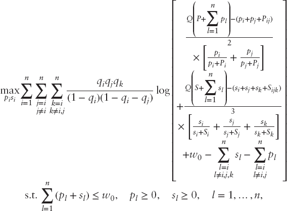
The effect of transactions costs, which is called slippage in commodity trading, is illustrated with the following place/show horseracing formulation; see Hausch, Ziemba, and Rubinstein (1981). Here, qi is the probability that i wins, and the Harville probability of an ij finish is ![]() , and so on. Q, the track payback, is about 0.82 (but is about 0.90 with professional rebates). The players’ bets are to place pj and show sk for each of the about 10 horses in the race out of the players’ wealth w0. The bets by the crowd are Pi with
, and so on. Q, the track payback, is about 0.82 (but is about 0.90 with professional rebates). The players’ bets are to place pj and show sk for each of the about 10 horses in the race out of the players’ wealth w0. The bets by the crowd are Pi with ![]() and Sk with
and Sk with ![]() . The payoffs are computed so that for place, the first two finishers, say i and j, in either order share the net pool profits once each Pi and pi bets cost of say $1 is returned. The show payoffs are computed similarly. The model is
. The payoffs are computed so that for place, the first two finishers, say i and j, in either order share the net pool profits once each Pi and pi bets cost of say $1 is returned. The show payoffs are computed similarly. The model is
While the Harville formulas make sense, the data indicate that they are biased. To correct for this, professional bettors adjust the Harville formulas, using for example discounted Harville formulas, to lower the place and show probabilities for favorites and raise them for the longshots; see papers in Hausch, Lo, and Ziemba (2008) and Hausch and Ziemba (2008).
This is a nonconcave program but it seems to converge when nonlinear programming algorithms are used to solve such problems. But a simpler way is via expected value approximation equations using thousands of sample calculations of the NLP model:
The expected value (and optimal wager) are functions of only four numbers—the totals to win and place for the horse in question. These equations approximate the full optimized optimal growth model. See Hausch and Ziemba (1985). This is used in calculators. See the discussion in Ziemba (2015).
An example is the 1983 Kentucky Derby (Figure 7.26).

Here, Sunny's Halo has about one-sixth of the show pool versus a quarter of the win pool, so the expected value is 1.14 and the optimal Kelly bet is 5.2 percent of one's wealth.
SOME GREAT INVESTORS
This portfolio optimization survey now shows the wealth plots of a number of great investors who have successfully used the Kelly and fractional Kelly strategies. These include John Maynard Keynes at King's College, University of Cambridge, Warren Buffett of Berkshire Hathaway, Bill Benter, the top racetrack bettor in Hong Kong, Ed Thorp, Princeton Newport, and Jim Simons of Renaissance Medallion (Figure 7.27).
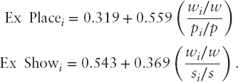
Ziemba (2005) argues that a modification of the Sharpe ratio is needed to evaluate properly the great investors, as the ordinary Sharpe ratio,

penalizes gains. See also the updated paper by Gergaud and Ziemba (2012). The modified measure uses only losses in the calculation of σP; namely,
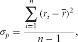

FIGURE 7.27 Four Great Investors: (a) John Maynard Keynes, King's College, Cambridge, 1927–1945; (b) Bill Benter, 1989–1991; (c) Ed Thorp, Princeton Newport Hedge Fund 1969–1988; (d) Jim Simons, Renaissance Medallion Hedge Fund, 1993–2005.
where r = 0 and ( )—means only the losses are counted. Using this measure, only Buffett improves on his Sharpe ratio as shown in Table 7.13. But Buffett is still below the Ford Foundation and the Harvard endowment with DSSRs near 1.00. The reason for that can be seen in Figure 7.28 where Berkshire has the highest monthly gains but also the largest monthly losses of the funds studies. It is clear that Warren Buffett is a long-term Kelly type investor who does not care about monthly losses, just high final wealth. The great hedge fund investors Thorp at DSSR = 13.8 and Simons at 26.4 dominate dramatically. In their cases, the ordinary Sharpe ratio does not show their brilliance. For Simons, his Sharpe was only 1.68.
Simons's wealth graph is one of the best I have seen (see Figure 7.14 and Table 7.14 for the distribution of his gains and losses). Renaissance Medallion has had a remarkable record: a net of 5 percent management fees and 44 percent incentive fees, so the gross returns are about double these net returns (Figure 7.29). Thorp's returns (Figure 7.27c) are with 2+20 fees and are a model for successful hedge fund performance with no yearly or quarterly losses and only three monthly losses in 20 years. See Gergaud and Ziemba (2012) for some funds with even higher DSSRs and one whose results are too good to be true with an infinity DSSR. That one turned out to be a Madoff-type fraud!

FIGURE 7.28 The wealth paths and return distributions of Berkshire Hathaway, Quantum, Tiger, Windsor, the Ford Foundation, and the S&P500, 1985–2000: (a) Growth of assets, log scale, various high performing funds, 1985–2000.
Source: Ziemba (2003); (b) Return distributions of all the funds, quarterly returns distribution, December 1985 to March 2000. Source: Ziemba (2005)
TABLE 7.13 Comparison of Ordinary and Symmetric Downside Sharpe Yearly Performance Measures, Monthly Data, and Arithmetic Means.
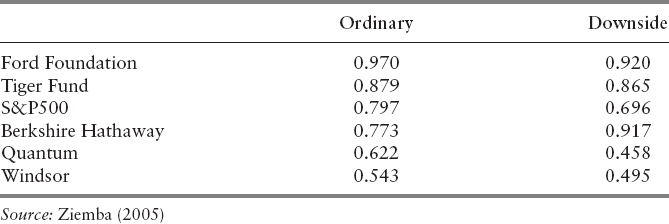


FIGURE 7.29 Medallion Fund, January 1993 to April 2005: (a) Rates of return in increasing order by month, %; (b) Wealth over time.
APPENDIX 7.1: ESTIMATING UTILITY FUNCTIONS AND RISK AVERSION
Certainty Equivalent Method

The three points plus the 0, 1 point generate u

Split each range one more to generate nine points.
For Donald Hausch, see Figure 2 these values were
Gain and Loss Equivalent Method
- Consider the gambles

or

x0 is the gain that would make the subject indifferent to a choice between A and B (gain equivalence)

Set
 .
.Hence this yields u(w0 + x0).
- Repeat with probability of winning = 0.2, 0.3, 0.4, 0.6, and 0.8.
- Consider the gambles

or

- Repeat with probability of winning = 0.2, 0.3, 0.4, 0.6, and 0.8.
For Donald Hausch, these values were

Points determined by 1, 2 are above (w0 + 5000) and by 3, 4 are below; see Figure 7.2.
Kallberg and Ziemba (1983) Method
Kallberg and Ziemba showed that the average Arrow Pratt risk aversion approximates closely the optimal Rubinstein measure under normality assumptions. So a consequence is that one can devise risk attitude questions to determine if a particular investor is a RA = 4 (pension fund investor 60–40 mix type) or a risk taker RA = 2 or a conservative investor RA = 6. Kallberg and Ziemba show that the accuracy of such questions is most crucial when RA is low; see Figure 7.30. The Chopra and Ziemba (1993) results discussed above are consistent with this.
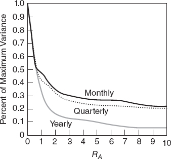
FIGURE 7.30 Riskiness as a percentage of maximum variance versus RA.
Source: Kallberg and Ziemba, 1983
REFERENCES
Algoet, P. H., and T. Cover. 1988. Asymptotic optimality and asymptotic equipartition properties of log-optimum investment. Annals of Probability 16 (2): 876–898.
Arrow, K. J. 1965. Aspects of the theory of risk bearing. Technical report. Helsinki: Yrjo Jahnsson Foundation.
Breiman, L. 1961. Optimal gambling system for favorable games. Proceedings of the 4th Berkeley Symposium on Mathematical Statistics and Probability 1: 63–8.
Brennan, M. J., and E. S. Schwartz 2008. The use of treasury bill futures in strategic asset allocation programs, in: W. T. Ziemba, and J. M. Mulvey. 2008, Worldwide Asset and Liability Modeling. Cambridge University Press, Cambridge, UK: 205–228.
Chopra, V. K. 1993. Improving optimization. Journal of Investing, 51–59.
Chopra, V. K., and W. T. Ziemba. 1993. The effect of errors in mean, variance and covariance estimates on optimal portfolio choice. Journal of Portfolio Management 19: 6–11.
Dantzig, G. 1955. Linear programming under uncertainty. Management Science 1: 197–206.
Fleten, S.-E., K. Høyland, and S. Wallace. 2002. The performance of stochastic dynamic and fixed mix portfolio models. European Journal of Operational Research 140 (1): 37–49.
Gassman, H. I., and W. T. Ziemba, eds. 2012. Stochastic Programming Applications in Finance, Energy and Production. Singapore: World Scientific.
Gergaud, O., and W. T. Ziemba. 2012. Evaluating great traders. Journal of Portfolio Management, Summer: 128–147.
Geyer, A., Herold, K. Kontriner, and W. T. Ziemba. 2002. The Innovest Austrian pension fund financial planning model InnoALM. Working paper, UBC.
Geyer, A., and W. T. Ziemba. 2008. The Innovest Austrian pension fund planning model InnoALM. Operations Research 56: 797–810.
Gondzio, J., and R. Kouwenberg. 2001. High performance computing for asset liability management. Operations Research 49: 879–891.
Grinold, R. C., and R. N. Khan. 1999. Active Portfolio Management: Quantitative Theory and Applications. New York: McGraw-Hill.
Guerard, J., ed. 2010. Ideas in Asset Liability Management in the Tradition of H. M. Markowitz in Essays in Honor of H. M. Markowitz. New York: Springer.
Hakansson, N. H. 1972. On optimal myopic portfolio policies with and without serial correlation. Journal of Business 44: 324–334.
Hakansson, N. H., and W. T. Ziemba. 1995. Capital growth theory. In Finance Handbook, edited by R. A. Jarrow, V. Maksimovic, and W. T. Ziemba, pp. 123–144. Amsterdam: North Holland.
Hanoch, G., and H. Levy. 1969. The efficiency analysis of choices involving risk. Review of Economic Studies 36: 335–346.
Hausch, D. B., V. Lo, and W. T. Ziemba, eds. 2008. Efficiency of Racetrack Betting Markets, 2nd ed. Academic Press, World Scientific.
Hausch, D. B., and W. T. Ziemba. 1985. Transactions costs, entries, and extent of inefficiencies in a racetrack betting model. Management Science XXXI: 381–394.
_________. (2008). Handbook of Sports and Lottery Markets. Amsterdam: North Holland
Hausch, D. B., W. T. Ziemba, and M. E. Rubinstein. 1981. Efficiency of the market for racetrack betting. Management Science XXVII: 1435–1452.
Kallberg, J. G., and W. T. Ziemba. 1981. Remarks on optimal portfolio selection. In Methods of Operations Research, Oelgeschlager, edited by G. Bamberg and O. Opitz, Vol. 44, pp. 507–520. Cambridge, MA: Gunn and Hain.
_________. 1983. Comparison of alternative utility functions in portfolio selection problems. Management Science 29 (11): 1257–1276.
_________. 1984. Mis-specifications in portfolio selection problems. In Risk and Capital, edited by G. Bamberg and K. Spremann, pp. 74–87. New York: Springer Verlag.
Lintner, J. 1965. The valuation of risk assets and the selection of risky investment in stock portfolios and capital budgets. Review of Economics and Statistics 47: 13–37.
Luenberger, D. G. 1993. A preference foundation for log mean-variance criteria in portfolio choice problems. Journal of Economic Dynamics and Control 17: 887–906.
_________. 1998. Investment Science. Oxford University Press.
MacLean, L., R. Sanegre, Y. Zhao, and W. T. Ziemba. 2004. Capital growth with security. Journal of Economic Dynamics and Control 38 (5): 937–954.
MacLean, L., W. T. Ziemba, and Li. 2005. Time to wealth goals in capital accumulation and the optimal trade-off of growth versus securities. Quantitative Finance 5 (4): 343–357.
MacLean, L. C., E. O. Thorp, Y. Zhao, and W. T. Ziemba. 2012. How does the Fortunes Formula-Kelly capital growth model perform? Journal of Portfolio Management 37 (4): 96–111.
MacLean, L. C., and W. T. Ziemba. 2006. Capital growth theory and practice. In S. A. Zenios and W. T. Ziemba (eds.), Handbook of asset and liability management, Volume 1, Handbooks in Finance, pp. 139–197. North Holland.
MacLean, L. C., and W. T. Ziemba, eds. 2013. Handbook of the Fundamentals of Financial Decision Making. Singapore: World Scientific.
Mangasarian, O. L. 1969. Nonlinear programming. New York: McGraw-Hill.
Markowitz, H. M. 1952. Portfolio selection. Journal of Finance 7 (1): 77–91.
_________. 1976. Investment for the long run: New evidence for an old rule. Journal of Finance 31 (5): 1273–1286.
_________. 1987. Mean-variance analysis in portfolio choice and capital markets. Cambridge, MA: Basil Blackwell.
Markowitz, H. M., and E. van Dijk. 2006. Risk-return analysis. In S. A. Zenios and W. T. Ziemba (Eds.), Handbook of asset and liability management, Volume 1, Handbooks in Finance. Amsterdam: North Holland, 139–197.
Merton, R. C., and P. A. Samuelson. 1974. Fallacy of the log-normal approximation to optimal portfolio decision-making over many periods. Journal of Financial Economics 1: 67–94.
Mossin, J. 1966. Equilibrium in a capital asset market. Econometrica 34 (October): 768–783.
_________. 1968. Optimal multiperiod portfolio policies. Journal of Business 41: 215–229.
Mulvey, J. M. 1996. Generating scenarios for the Towers Perrin investment system. Interfaces 26: 1–13.
Mulvey, J. M., and B. Pauling. 2002. Advantages of multi-period portfolio models. Journal of Portfolio Management 29: 35–45.
Mulvey, J. M., B. Pauling, S. Britt, and F. Morin. 2007. Dynamic financial analysis for multinations insurance companies. In Handbook of asset and liability management, Volume 2, Handbooks in Finance edited by S. A. Zenios and W. T. Ziemba. Amsterdam: North Holland, 543–590.
Murty, K. G. 1972. On the number of solutions to the complementarity problem and spanning properties of complementarity cones. Linear Algebra 5: 65–108.
Pratt, J. W. 1964. Risk aversion in the small and in the large. Econometrica 32: 122–136.
Rockafellar, T., and W. T. Ziemba. 2013, July. Modified risk measures and acceptance sets. in The Handbook of the Fundamentals of Financial Decision Making edited by L. C. MacLean and W. T Ziemba, Vol. II: 505–506.
Samuelson, P. A. 1969. Lifetime portfolio selection by dynamic stochastic programming. Review of Economics and Statistics 51: 239–246.
_________. 1971. The fallacy of maximizing the geometric mean in long sequences of investing or gambling. Proceedings National Academy of Science 68: 2493–2496.
_________. 2006. Letter to W. T. Ziemba, December 13.
_________. 2007. Letter to W. T. Ziemba, May 7.
Sharpe, W. F. 1964. Capital asset prices: A theory of market equilibrium under conditions of risk. Journal of Finance 19: 425–442.
Siegel, J. 2008. Stocks for the Long Run, 4th ed. New York: McGraw-Hill.
Thorp, E. O. 2006. The Kelly criterion in blackjack, sports betting and the stock market. In Handbook of asset and liability management, Handbooks in Finance, edited by S. A. Zenios and W. T. Ziemba, pp. 385–428. Amsterdam: North Holland.
Tobin, J. 1958. Liquidity preference as behavior towards risk. Review of Economic Studies 25 (2): 65–86.
Wallace, S. W., and W. T. Ziemba, eds. 2005. Applications of Stochastic Programming. SIAM—Mathematical Programming Society Series on Optimization.
Zangwill, W. I. 1969. Nonlinear Programming: A Unified Approach. Englewood Cliffs, NJ: Prentice Hall.
Ziemba, R. E. S., and W. T. Ziemba. 2007. Scenarios for Risk Management and Global Investment Strategies. New York: John Wiley & Sons.
Ziemba, W. T. 2015. Exotic betting at the racetrack. Singapore: World Scientific.
Ziemba, W. T. 1974. Calculating investment portfolios when the returns have stable distributions. In Mathematical Programming in Theory and Practice, edited by P. L. Hammer and G. Zoutendijk, pp. 443–482. Amsterdam: North Holland.
_________. 2003. The stochastic programming approach to asset liability and wealth management. Charlottesville, VA: AIMR.
_________. 2005. The symmetric downside risk Sharpe ratio and the evaluation of great investors and speculators. Journal of Portfolio Management, Fall: 108–122.
_________. 2007. The Russell–Yasuda Kasai InnoALM and related models for pensions, insurance companies and high net worth individuals. In Handbook of asset and liability management, Volume 2, Handbooks in Finance, edited by S. A. Zenios and W. T. Ziemba, pp. 861–962. Amsterdam: North Holland.
_________. 2013. The case for convex risk measures and scenario dependent correlation matrices, Quantitative Finance Letters 1: 47–54.
Ziemba, W. T., and D. B. Hausch. 1986. Betting at the Racetrack. Dr. Z Investments, Inc., San Luis Obispo, CA.
Ziemba, W. T., and J. M. Mulvey. 2008. Worldwide Asset and Liability Modeling. Cambridge University Press, Cambridge, UK.
Ziemba, W. T., C. Parkan, and F. J. Brooks-Hill. 1974. Calculation of investment portfolios with risk free borrowing and lending. Management Science XXI: 209–222.
Ziemba, W. T., and R. G. Vickson, eds. 1975. Stochastic Optimization Models in Finance. New York: Academic Press. Reprinted (2006) with a new preface. Singapore: World Scientific.