CHAPTER 6

Risk Measures and Management in the Energy Sector

Marida Bertocchi
Rosella Giacometti
Maria Teresa Vespucci

University of Bergamo¹, Department of Management, Economics, and Quantitative Methods

INTRODUCTION

As a result of the liberalization of energy markets, energy companies got an increased understanding of the need both of profit maximization and of considering the risks connected with their activities as well as the way of hedging them; they also became aware of their own different level of risk aversion policies. In energy-sector modeling, dealing with uncertainty is a part of the problem, as well as with making decisions in different points in time. These two characteristics bring the energy sector modeling in the stochastic programming framework. The two issues of risks and decisions under uncertainty support the choice of having multistage type stochastic programs (see Ruszczynski and Shapiro, 2003; Shapiro, Dentcheva, and Ruszczynski, 2009).

In this chapter we illustrate two problems in the energy sector where the awareness of risk is fundamental, and we analyze the main advantages of introducing risk management in our models.

The first problem is related to power production and electricity trading. There is an extensive literature dealing with optimization of power production and electricity trading. See Alonso-Ayuso, di Domenica, Escudero, and Pizarro (2011), Conejo, Carrion, and Morales (2010), Fleten and Wallace (1998, 2009), Fleten and Kristoffersen (2008), Gröwe-Kuska, Kiwiel, Nowak, Römisch, and Wegner (2002), and Takriti, Krasenbrink, and Wu (2000). In this framework, risk management becomes a significant issue for electricity retailers and producers, and contracts for future delivery of electricity (i.e., forwards contracts) become a tool for hedging risk. Indeed, the retailers are highly constrained by regulated tariff consumers, and they are subject to risk of high electricity price. We show a comparison between deterministic and stochastic models able to optimally solve the problem.

The second problem concerns the incremental selection of power generation capacity, which is of great importance for energy planners. In this chapter, we deal with the case of the single power producer's (GenCo) point of view. That is, we want to determine the optimal mix of different technologies for electricity generation, ranging from coal, nuclear, and combined cycle gas turbine to hydroelectric, wind, and photovoltaic, taking into account the existing plants, the cost of investment in new plants, the maintenance costs, the purchase and sales of CO₂ emission trading certificates, and renewable energy certificates (RECs, or green certificates) to satisfy regulatory requirements over a long-term planning horizon consisting of a set I of years (generally, 30 or more years). Uncertainty of prices (fuels, electricity, CO₂ emission permits, and green certificates) is taken into account. The power producer is assumed to be a price taker; that is, it cannot influence the price of electricity.

We propose various models for maximizing the net present value of the power producer's profit, in order to find an optimal trade-off between the expected profit (should it be the unique term in the objective function to maximize, it is so named risk-neutral strategy) and the risk of getting a negative impact on the solution's profit due to a not-wanted scenario to occur. So this weighted mixture of expected profit maximization and risk minimization undoubtedly may be perceived as a more general model than the levelized cost of energy (LCoE) procedure (Manzhos, 2013). See some similar approaches in Bjorkvoll, Fleten, Nowak, Tomasgard, and Wallace (2001), Eppen, Martin, and Schrage (1989), Genesi, Marannino, Montagna, Rossi, Siviero, Desiata, and Gentile (2009), Cristobal, Escudero, and Monge (2009), and Escudero, Garin, Merino, and Perez (2012), Ehrenmann and Smeers (2011), among others. The main contribution of the proposed model is the provisions of consistent solutions, since for all of them the optimal generation mix mainly consists of conventional thermal power plants for low risk aversion, which are replaced by renewable energy sources plants as risk aversion increases.

UNCERTAINTY CHARACTERIZATION VIA SCENARIOS

Decision-making problems related to electricity markets are characterized by uncertainty. The input data of problems affected by uncertainty are usually described by stochastic processes that can be represented using continuous or discrete random variables.

The most used case is the one of discrete stochastic process that can be represented by a finite set of vectors, named scenarios, obtained by all possible discrete values that the random variables can assume.

If μ is a discrete stochastic process, it can be expressed as μ_ω, with ω the scenario index and Ω the finite number of scenarios. Each scenario has a certain probability p_ω of occurrence with

The scenario generation procedure may use time series analysis, statistical, and econometric modeling for the forecasting of future values of the random variables, experts opinion, and simple possible outcomes.

In the problems described in this chapter we study the following sources of uncertainty: the spot price of energy, the forward price of energy, the fuel prices, CO₂ and green certificate prices. Other sources of variability may involve inflows for hydropower plants (see Fleten and Wallace 2009), intensity of wind, demand (see Philpott, Craddock, and Waterer 2000), and many others (see Eppen, Martin, and Schrage 1989, and references therein).

For a general discussion about the procedures for generating scenarios in a multistage stochastic program, see Dupačová, Consigli, and Wallace (2000).

Spot and Forward Prices of Energy

Concerning the spot price of energy, the Italian electricity spot market was opened in 2003, and its activity has been increasing during the last years and it is considered a liquid market with many daily transactions. In our analysis we consider the daily base-load spot prices time series from January 1, 2008, to September 9, 2009. After removing the daily and weekly seasonal components, we analyzed the log prices data and found stationarity but no strong presence of spikes: only four observations are larger then three times the standard deviation on the whole period. The log spot price exhibits autocorrelation and heteroskedasticity but not a dramatic kurtosis. In line with recent findings in literature, we fit a regime-switching model able to capture different market conditions, in terms of changing mean and volatilities. For details on the AR(1) model used in fitting the log price process and the Markov chain model used for the switching model, see Giacometti, Vespucci, Bertocchi, and Barone Adesi (2011; 2013).

Using the complete data set, we find the evidence of the presence of two regimes (see Figure 6.1).

We have derived the theoretical dynamics of the forward prices by directly modeling them. The motivation of this approach is that, in reality, the electricity spot and futures prices are not closely related. This is mainly due to the difficulty in storing electricity. Water reservoirs can be used for storing potential energy in limited quantities due to the their physical limited capacity. Often, the spot and futures markets are so dissimilar that the relationship between spot and futures prices breaks down. If we compare, ex post, the forward quotations with the realized spot prices, we observe that the difference does not necessarily tend to zero for contracts approaching their maturity; see also Borovkova and Geman (2006; 2006), where they indicate that the futures price is a poor proxy for the electricity spot price. For this reason we have modeled explicitly the dynamics of the forward curve, imposing that the scenarios generated for the spot and forward contracts are correlated and consistent with the currently observed contract quotations.

The procedure used for scenario generation involves two distinct steps. By principal component analysis (PCA) on the daily deseasonalized historical returns of forward key rates, we compute the orthogonal factors: the first three factors explain 92 percent of the forward curve and correspond to a parallel shift (first factor, which explains 61 percent), a tilting (second factor, which explains 17 percent), and a curvature effect (third factor explains 14 percent).

We consider as relevant the first two factors that have an explanatory power of about 80 percent of the variability.

The residuals contain all the information related to the remaining 20 percent of variability and the correlation among the returns of the different maturities. We model the variance of the residuals with a univariate GARCH(1,1) model in order to capture the dependence of returns.

In order to generate correlated scenarios, we combine together the standardized residuals of the GARCH(1,1) model and the residuals from the regime-switching model for the same days. We do not impose any parametric assumption on the marginal distributions and use the empirical cumulative distribution to fit a Gaussian copula of the historical residuals vectors. We simulate a vector of correlated innovations from the Gaussian copula and reconstruct the forecasted scenarios using the estimated principal factors for the forward return scenario and the regime switching for the log spot price, finally adding the seasonal premia.

To build the scenario tree for the three-stage stochastic programming model, we first generate 100 correlated scenarios for spot and forward prices on a time horizon of one year, and then we aggregate them in a recombining tree using the backward scenario reduction technique proposed by Pflug (2001) and Pflug and Hochreiter (2007). In order to maintain consistency with the market, the spot price scenarios were adjusted so that the expected average spot price in a period is equal to the current market price of a forward with delivery in that period. To avoid arbitrage opportunities, we impose that spot price tree satisfies the martingale property in the recombining tree.

Fuel Prices

Tables 6.1 and 6.2 provide six alternative values of the ratio “estimated price over price in year 0” that are considered, together with the associated probabilities for coal and gas, respectively. Analogously, Table 6.3 provides three alternative values and the associated probabilities for nuclear fuel. By combining all alternatives, 108 independent scenarios of fuel prices are obtained.

As the number of scenarios is increased, the 0-1 variables, necessary for modeling the risk measures shortfall probability and first-order stochastic dominance, substantially increase the computing time, and decomposition algorithms have to be used for obtaining the solution in a reasonable computing time. This problem does not arise in the case reported in this chapter using CVaR risk measure.

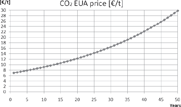
The price of the CO₂ emission allowances is assumed to increase along the years of the planning horizon. We consider only one scenario; see Figure 6.3.

The ratio “electricity from RES / total electricity produced” is set according to the 20-20-20 European target from year 2011 to year 2020 (i.e., from year 1 to year 8 of the planning period); after 2020, a further increase of 1 percent is assumed.

The GenCo can satisfy the imposed ratio by either producing from RES or buying green certificates.

MEASURES OF RISKS

Being F_ω the value of profit function along scenario ω ∈ Ω, the risk-neutral approach determines the values of the decision variables that maximize, over all scenarios, the expected profit ∑_ω∈Ωp_ωF_ω along the planning horizon. This type of modeling does not take into account the variability of the objective function value over the scenarios and, then, the possibility of realizing in some scenarios a very low profit. In the literature, several approaches have been introduced for measuring the profit risk. These measures can be divided into four groups, on the basis of the information the user must provide:

1. A form for the cardinal utility: expected utility approach
2. A confidence level: value-at-risk and conditional-value-at-risk
3. A profit threshold: shortfall probability and expected shortage
4. A benchmark: first-order and second-order stochastic dominance

In this section we consider these risk measures and how they can be used to reduce the risk of having low profits in some scenarios. To see the use of all of them in the power-capacity planning problem, see Vespucci, Bertocchi, Pisciella, and Zigrino (2014).

Risk Aversion Strategy 1: The Expected Utility Approach

The expected utility approach is based on the famous theorem from Von Neumann and Morgenstern (1944). It states that given two probability distributions G_a and G_b of the random variables respectively a and b representing decisions, satisfying axioms of completeness, transitivity, continuity, and independence of preference relation among distributions, there exists a utility function (the expected utility function) U : R → R such that , where V : F → R is the ordinal utility defined on the set F of distributions, and x_i represents the ith realization of random variable a with probability p_a,i. The argument of function U is quite often the wealth of the individual.

Two further axioms of nonsatiability and risk aversion are usually required on U: the former states that one requires more than less, and the latter states that the utility of the expected value of a random variable is greater than the expected value of the utility function of the same variable. It is easy to show that the risk aversion property is equivalent to require the concavity of function U or that the certainty equivalent is less than the expected value of the random variable.

There are various forms of the utility function that exhibit different characteristics: among them the most famous are the quadratic function that corresponds to having a normal distribution of the random variable, the negative exponential that exhibits constant absolute risk aversion, and the power utility with constant relative risk aversion.

Risk Aversion Strategy 2: Conditional Value at Risk (CVaR)

The CVaR of profits is defined as the expected value of the profits smaller than the α-quantile of the profits distribution—that is, it is the expected profit in the α percentage of the worst scenarios; see Conejo, Carrion, Morales (2010). We observe that increasing value of CVaR means decreasing risk.

Given the confidence level α, the CVaR of profit (see Gaivoronski and Pflug 2005; Rockafellar and Uryasev 2000, 2002; Schultz and Tiedemann, 2006) is defined as

The auxiliary variables V [k€] and d_ω [k€], ω ∈ Ω, used for computing the CVaR, are defined by constraints

and V is the optimal solution representing the value at risk (VaR).

In order to use the CVaR of profit as a risk-aversion strategy, the objective function can be expressed

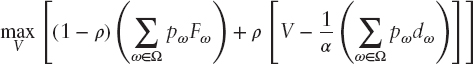
where ρ ∈ [0, 1] is the CVaR risk-averse weight factor, ρ = 0 means to consider the risk-neutral case, ρ = 1 means maximum risk aversion. In a different context, see Alonso-Ayuso, di Domenica, Escudero, and Pizarro (2011); Cabero, Ventosa, Cerisola, and Baillo (2010); and Ehrenmann, and Smeers (2011).

Risk Aversion Strategy 3: Shortfall Probability (SP)

Given a profit threshold Φ, the shortfall probability (see Schultz and Tiedemann 2006) is the probability of the scenario to occur having a profit smaller than Φ:

where μ_ω is a 0-1 variable defined by the constraint

where variable μ_ω takes value 1 if F_ω < Φ, that is, if ω is an unwanted scenario, and M_ω is a small enough constant such that it does not prevent any feasible solution to the problem, being this parameter crucial for the computational effort required to obtain the optimal solution.

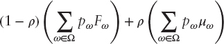
The profit risk can be hedged by simultaneously pursuing expected profit maximization and shortfall probability minimization: this is done by maximizing the objective function, with ρ ∈ [0, 1],

subject to constraints related to the modeled problem and constraints (6.1).

Risk Aversion Strategy 4: Expected Shortage (ES)

Given a profit threshold Φ, the expected shortage (see Eppen, Martin, and Schrage 1989) is given by

where d_ω satisfies constraint

The profit risk can be hedged by simultaneously pursuing expected profit maximization and expected shortage minimization: This is done by maximizing the objective function, with ρ ∈ [0, 1],

subject to constraints related to the modeled problem and constraints (6.2).

Risk Aversion Strategy 5: First-Order Stochastic Dominance (FSD)

A benchmark is given by assigning a set P of profiles (Φ^p, τ^p), p ∈ P, where Φ^p is the threshold to be satisfied by the profit at each scenario and τ^p is the upper bound of its failure probability.

The profit risk is hedged by maximizing the expected value of profit, while satisfying constraints related to the modeled problem, as well as the first-order stochastic dominance constraints; see Carrion, Gotzes, and Schultz (2009) and Gollmer, Neise, and Schultz (2008):

where the 0-1 variables by which the shortfall probability with respect to threshold Φ^p is computed are defined by constraints

with

Constraints (6.3) and (6.4) belong to the cross-scenario constraint type, and they introduce an additional difficulty in the decomposition algorithms. See in Escudero, Garin, Merino, and Perez (2012) a multistage algorithm for dealing with this type of constraints.

Risk Aversion Strategy 6: Second-Order Stochastic Dominance (SSD)

A benchmark is assigned by defining a set of profiles (Φ^p, e^p), p ∈ P, where Φ^p denotes the threshold to be satisfied by the profit at each scenario and e^p denotes the upper bound of the expected shortage over the scenarios. The profit risk is hedged by maximizing the expected value of profit, while satisfying constraints related to the modeled problem as well as the second-order stochastic dominance constraints (see Gollmer, Gotzes, and Schultz, 2011):

where

with

This measure is closely related to the risk measure introduced in Fabian, Mitra, Roman, and Zverovich (2011), where the threshold p ∈ P is considered as the benchmark. In a different context, see also Cabero, Ventosa, Cerisola, and Baillo (2010).

Notice that constraints (6.5) and (6.6) are also cross-scenario constraints, but the related variables are continuous ones.

It is interesting to point out that the risk-aversion strategies FSD and SSD have the advantage that the expected profit maximization is hedged against a set of unwanted scenarios: The hedging is represented by the requirement of forcing the scenario profit to be not smaller than a set of thresholds, with a bound on failure probability for each of them in strategy FSD and an upper bound on the expected shortage in strategy SSD. The price to be paid is the increase of the number of constraints and variables (being 0-1 variables in strategy FSD).

For large-scale instances, decomposition approaches must be used, like the exact multistage Branch-and-Fix Coordination (BFC-MS) method (Escudero, Garin, Merino, and Perez, 2012), currently being expanded to allow constraint types (FSD) and (SSD) (Escudero, Garin, Merino, and Perez 2012a); multistage metaheuristics, like Stochastic Dynamic Programming (Cristobal, Escudero, and Monge 2009; Escudero, Monge, Romero-Morales, and Wang 2012), for very large scale instances; and Lagrangian heuristic approaches, see (Gollmer, Gotzes, and Schultz 2011).

Notice that both FSD and SSD strategies require the determination of benchmarks, which may require computing time consumption.

CASE STUDIES

Forward Markets Trading for Hydropower Producers

For a hydropower producer, on a yearly horizon, it is very important to identify the optimal scheduling of its production in order to satisfy a production profile that may be particularly difficult to match in some months of the year. The production profile is the forecast of customers’ energy demand. The use of derivative contracts may help to optimize the hydro resources.

The hydropower producer's portfolio includes its own production, a set of power contracts for delivery or purchase including derivative contracts, like options, futures or forwards with physical delivery, to hedge against various types of risks. In this subsection, we summarize deterministic and stochastic portfolio models for a hydropower producer operating in a competitive electricity market. For detailed description of the models see Giacometti, Vespucci, Bertocchi, and Barone Adesi (2011; 2013).

The novelty of our approach consists in a more detailed modeling of the electricity derivatives contracts, leading to an effective daily hedging.

The goal of using such a model is to reduce the economic risks connected to the fact that energy spot price may be highly volatile due to various different, unpredictable reasons (i.e., very cold winter) and to the possibility of a scarcity of rain or melting snow. Indeed, the use of forward contracts in a dynamic framework is expensive, but relying on the energy spot market may be extremely risky. See Dentcheva and Römisch (1998), Gröwe-Kuska, Kiwiel, Nowak, Römisch, and Wegner (2002), Wallace, and Fleten (2003), Fleten and Kristoffersen (2008), Conejo, Garcia-Bertrand, Carrion, Caballero, and de Andres (2008) and Nolde, Uhr, and Morari (2008) for discussion on the opportunity of using stochastic programming for such problems and Yamin (2004) for a review of methods for power-generation scheduling.

The basis risk factors include the wholesale spot and forward prices of electric energy, which are supposed to be unaffected by the decision of the utility manager, and the uncertain inflow of hydro reservoirs; see also Fleten and Wallace (2009), Vitoriano, Cerisola, and Ramos (2000), and Latorre, Cerisola, and Ramos (2007). The model we propose differs from the one discussed in Fleten and Wallace (1998; 2009), as we concentrate on the advantage of using derivatives contracts and use both electricity spot prices and forward prices as sources of uncertainties, considering inflows as deterministic. The objective function is the expected utility function of the final wealth, where the cardinal utility is a power function with constant relative risk aversion equal to 0.5.

We report the results of a comparison of deterministic and stochastic approaches in the case of an hydro system composed by one cascade with three basins and three hydro plants, one of these is a pumped storage hydro plant as shown in Figure 6.4 (see Tables 6.4 and 6.5 for input data of the hydro system).

The model has been used on a yearly horizon considering only working days. In order to represent the scenarios we introduce the following notation to indicate the number of days included in the different stages (see also Vespucci, Maggioni, Bertocchi, Innorta, 2012): T₁ = 1, T₂ = {t : 2 ≤ t ≤ 20}, T₃ = {t : 21 ≤ t ≤ 191}, where the subindexes indicate the stage. We have considered 25 scenarios represented by means of a scenario tree where the nodes at different stages are as follows: N₁ = 1, N₂ = {2, …, 6}, N₃ = {7, …, 31}.

In order to assess the value of modeling uncertainty for our three-stage model, we follow the procedure introduced in the literature by Escudero, Garin, and Perez (2007), and Vespucci, Maggioni, Bertocchi, and Innorta (2012), for evaluating the value of the stochastic solution for three-stage problem, and further deepened in Maggioni, Allevi, and Bertocchi (2012) and Maggioni, Allevi, and Bertocchi (2013).

The procedure is based on the idea of reproducing the decision process as the uncertainty reveals: This procedure is suitable for multistage problems.

The optimal objective value obtained in stage 3 is called multistage expected value of the reference scenario (MEVRS), where the reference scenario is the mean value scenario.

Technically, this is computed by the following steps:

1. Scenario tree S_(1,mean) is defined by considering the expected value of the uncertainty parameters (spot and forward prices); the stochastic model with this scenario tree is solved and the optimal values of the first-stage variables are stored. In this way, the optimal solution of the expected mean value (EV) problem is computed.
2. Scenario tree S_(2,mean) is defined by evaluating the expected value of the spot and forward prices on nodes belonging to N₃. The stochastic model with this scenario tree is solved having assigned the value stored at step 1 to the first-stage decision variables. The optimal value of second-stage variables are stored.
3. The stochastic model on benchmark tree S_(1,mean) is solved, assigning to the first-stage decision variables the values stored at step 1 and to the second-stage decision variables the values stored at step 2.

We report the results considering all the sources of variability, the spot and the forward prices. The use of forward contracts allows a more efficient use of water pumping with a higher final level of water in the basins.

Overall, the effects of the financial part and the production scheduling lead to an increase in the objective function, from 232,068.61 to 251,308.03 €. We report the certainty equivalent related to the previously mentioned utility function.

We observe in Table 6.6 that the value of the objective function (EV value) using the respective average scenario of spot and forward prices (the deterministic case) is higher than in the stochastic solution. The stochastic approach, even with a limited number of scenarios obtained by a reduction technique (see Heitsch, and Römisch, 2007; 2009a; 2009b), allows the producer to better diversify its consecutive choices along the year, adapting the production and the protection against high energy price (i.e., the decision variables) according to the energy price changes along the different scenarios. In the deterministic approach, one cannot take into account different realizations of the random variables.

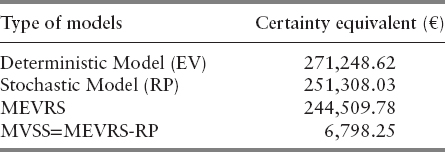
We also compute the multistage expected value of the mean value scenario MEVRS = 244, 509.78. The modified value of the stochastic solution (MVSS = MEVRS-RP) is 6,798.25, and it allows us to obtain the goodness of the expected solution value when the expected values are replaced by the random values for the input variables. High values of modified VSS indicate the advantage of using the stochastic approach with respect to the deterministic one.

Capacity Power Production Planning in the Long Run

We present a decision support model for a power producer who wants to determine the optimal planning for investment in power generation capacity in a long-term horizon. The power producer operates in a liberalized electricity market, where rules are issued by the regulatory authorities with the aim of promoting the development of power production systems with reduced CO₂ emissions. Indeed, CO₂ emission allowances have to be bought by the power producer as a payment for the emitted CO₂. Moreover, the green certificate scheme supports power production from renewable energy sources (RES)—that is, by geothermal, wind, biomass and hydropower plants—and penalizes production from conventional power plants such as CCGT, coal, and nuclear power plants. Indeed, every year a prescribed ratio is required between the electricity produced from RES and the total electricity produced. In case the actual ratio, attained in a given year, is less than the prescribed one, the power producer must buy green certificates in order to satisfy the related constraint. On the contrary, when the yearly attained ratio is greater than the prescribed one, the power producer can sell green certificates in the market.

The power producer aims at maximizing its own profit over the planning horizon. Revenues from sale of electricity depend both on the electricity market price and on the amount of electricity sold. The latter is bounded above by the power producer's market share; it also depends on the number of operating hours per year characterizing each power plant in the production system.

Costs greatly differ among the production technologies. Investment costs depend both on the plant-rated power and on the investment costs per power unit. Typically, for thermal power plants, rated powers are higher and unit investment costs are lower than for RES power plants. Variable generation costs for conventional power plants highly depend on fuel pricing.

Revenues and costs associated to the green certificate scheme depend on the green certificate price, as well as on the yearly ratio between production from RES and total annual production of the producer. Finally, costs for emitting CO₂ depend on the price of the emission allowances, as well as on the amount of CO₂ emitted, that greatly varies among the production technologies.

We notice that the evolution of prices along the planning horizon is not known at the time when the investment decisions have to be done. The model takes into account the risk associated with the capacity expansion problem due to the uncertainty of prices, as well as the uncertainty of market share. Uncertainty is included in the model by means of scenarios that represent different hypotheses on the future evolution of the market share and of the prices of electricity, green certificates, CO₂ emission allowances, and fuels.

The proposed decision support model determines the evolution of the production system along the planning horizon, taking into account all scenarios representing the uncertainty. Since construction time and industrial life greatly vary among power plants of different technology, the model determines the number of power plants for each technology to start construction in every year of the planning period. Each new power plant is then available for production when its construction is over and its industrial life is not ended. The annual electricity production of each power plant in the production system, and the corresponding green certificates and CO₂ emission allowances, are determined for each year of the planning horizon under each scenario into consideration.

The two-stage stochastic mixed-integer model determines the optimal generation expansion plan, which is given by the values of the first-stage variables

that represent the number of new power plants of technology j ∈ J where construction is to start in year i ∈ I along the planning horizon, being J the set of all candidate technologies, and I the set of years in the planning horizon. The second-stage variables are the continuous operation variables of all power plants along the time horizon.

The optimal generation expansion plan must satisfy the following constraints.

For every candidate technology j, the total number of new power plants constructed along the planning horizon is bounded above by the number of sites ready for construction of new power plants of that technology—that is, sites for which all the necessary administrative permits have been released. The new power plants of technology j available for production in year i are those for which both the construction is over and the industrial life is not ended.

The sum of the present annual debt repayments, corresponding to the number of new power plants of each technology j available for production in every year i, is required not to exceed the available budget.

The annual electricity production obtained by all new power plants of technology j is nonnegative and bounded above by the number of new plants available for production in year i times the maximum annual production of a plant of technology j.

The annual electricity production of power plant k ∈ K (K the set of all power plants owned in year 0) is nonnegative and bounded above by the maximum annual production in year i. Parameters are introduced to take into account possible plant breakdown and maintenance.

Notice that for some technologies a lower bound to the annual electricity production could be imposed, if it is selected, in order to take into account technical limitations.

The electricity generated in year i cannot exceed the power producer's market share under scenario w.

The amount of electricity G_i,w for which the corresponding green certificates are bought, if G_i,w ≥ 0, or sold, if G_i,w ≤ 0, in year i under scenario ω is used to take into account revenue or costs, depending on whether the energy production from renewable sources with respect to the total energy production is greater or less than the quantity β_i fixed by the regulatory authority.

The amount Q_i,w of CO₂ emissions the power producer must pay for in year i under scenario ω is computed by adding the emissions obtained by all the thermal plants (original and candidates).

The annual profit F_w under scenario ω is computed taking into account the revenues from sale of electricity, the revenues or costs of green certificates, the costs of CO₂ emission allowances, fixed and variable costs for thermal and RES production, and the annuity of investment costs.

The risk-neutral approach determines the values of the decision variables that maximize, over all scenarios, the expected profit along the planning horizon. It does not take into account the variability of the objective function value over the scenarios and, then, the possibility of realizing in some scenarios a very low profit.

In order to use the CVaR of profit as a risk-aversion strategy, the objective function has to be expressed:

where ρ ∈ [0, 1] is the CVaR risk averse weight factor.

We report the results obtained for a power producer who owns in year 0 the medium-size generation system described in Table 6.7, where rated power, residual life, and efficiency are reported for every power plant of the system. The generation system owned initially, with total capacity of 8,629 MW, is biased toward the CCGT technology and is therefore highly dependent on the gas price.

Let us consider a market electricity price of 106 €/MWh and two values for the initial budget, in order to show its influence on the technology mix. The confidence level α used to compute the CVaR is 5 percent.

For the case corresponding to the budget B = 3.84 G€, the profit distributions are shown in Figure 6.5.

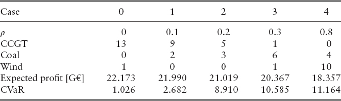
In Table 6.8 we can observe a regular change in the technology mix as the risk aversion parameter increases.

Notice the difference between the case with ρ = 0 (risk neutral) and the case with ρ = 0.2 (risk averse): The expected profit decreases by only 5 percent (1.154 G€), while the CVaR has grown by 9.926 G€.

By further increasing the risk aversion parameter (ρ = 0.3 and ρ = 0.8), the corresponding optimal technology mixes have a small growth of the CVaR but have a big decrease in the expected profit.

For the case with a higher budget, say 14.5 G€, the profit distributions are shown in Figure 6.6.

The nuclear technology appears in the mix (see Table 6.9) only with high risk aversion (ρ ≥ 0.5), and it represents a low percentage of the new capacity mix (see Figure 6.7).

With a budget lower than 14.5 G€, the nuclear technology is not included in the optimal mix, due to the rated power of nuclear plants.

Moreover, it can be seen in Figure 6.8 that for electricity prices less than 112 €/MWh, the LCoE associated to the nuclear technology is less than the LCoE associated to the wind power technology.

SUMMARY

In this chapter, we have explored the most important notions of risk in the energy sector, as well as the major sources of uncertainty from which risk is originating. We have described how to cope with these uncertainties by two main tools: construction of scenarios and stochastic programming modeling. The former has been achieved by using discrete stochastic processes, mainly GARCH processes. The latter has been attained by implementing a stochastic programming approach and analyzing the behavior of the solutions. Two relevant problems for the energy sector have been discussed:

1. A hydropower producer that wants to use the electricity forward market for hedging against the increase in electricity prices
2. The capacity power production planning in the long run for a single price-taker producer

We point out that one of the most promising research direction in the dynamic energy problems with embedded risk profile is the use of the discussed risk measures in the multistage framework instead of the two-stage one. This stimulating topic, which is at present under analysis within the financial research studies, implies a careful analysis of “consistent” risk measures to be used in energy problems.

REFERENCES

Alonso-Ayuso, A., N. di Domenica N., L.F. Escudero L.F., and C. Pizarro. 2011. Structuring bilateral energy contract portfolios in competitive markets. In Bertocchi M., Consigli G., Dempster M.A.H., Stochastic Optimization Methods in Finance and Energy. International Series in Operations Research and Management Science, New York: Springer Science + Business Media 163 (2): 203–226.

Björkvoll, T., S. E. Fleten, M.P. Nowak, A. Tomasgard, and S.W. Wallace. 2001. Power generation planning and risk management in a liberalized market, IEEE Porto Power Tech Proceeding 1: 426–431.

Borovkova, S., and H. Geman. 2006. Analysis and Modeling of Electricity Futures Prices Studies. Studies in Nonlinear Dynamics and Econometrics 10 (3): 1–14.

Borovkova, S., and H. Geman. 2006a. Seasonal and stochastic effects of commodity forward curve. Review of Derivatives Research 9 (2): 167–186.

Cabero, J., M. J. Ventosa, S. Cerisola, and A. Baillo. 2010. Modeling risk management in oligopolistic electricity markets: a Benders decomposition approach. IEEE Transactions on Power Systems 25: 263–271.

Carrion, M., U. Gotzes, and R. Schultz. 2009. Risk aversion for an electricity retailer with second-order stochastic dominance constraints. Computational Management Science 6: 233–250.

Conejo, A. J., M. Carrion, and J. M. Morales. 2010. Decision making under uncertainty in electricity market. International Series in Operations Research and Management Science. New York: Springer Science+Business Media.

Conejo, A. J., R. Garcia-Bertrand, M. Carrion, A. Caballero, and A. de Andres. 2008. Optimal involvement in future markets of a power producer. IEEE Transactions on Power Systems 23 (2): 703–711.

Cristobal, M. P., L. F. Escudero, and J. F. Monge. 2009. On stochastic dynamic programming for solving large-scale tactical production planning problems. Computers and Operations Research 36: 2418–2428.

Dentcheva, D., and W. Römisch. 1998. Optimal power generation under uncertainty via stochastic programming. Stochastic Programming Methods and Technical Applications, Lecture Notes in Economics and Mathematical Systems. New York: Springer 458: 22–56.

Dupačová, J., G. Consigli, and S.W. Wallace. 2000. Scenarios for multistage stochastic programs. Annals of Operations Research 100(1–4): 25–53.

Ehrenmann, A., and Y. Smeers. 2011. Stochastic equilibrium models for generation capacity expansion. In Stochastic Optimization Methods in Finance and Energy, edited by M. Bertocchi, G. Consigli, and M. A. H. Dempster. International Series in Operations Research and Management Science. New York: Springer Science + Business Media 163(2), 203–226.

Eppen, G. D., R. K. Martin, and L. Schrage. 1989. Scenario approach to capacity planning. Operations Research 34: 517–527.

Escudero, L. F., M. A. Garín, M. Merino, and G. Perez. 2012. An algorithmic frame-work for solving large scale multistage stochastic mixed 0-1 problems with nonsymmetric scenario trees, Computers and Operations Research 39: 1133–1144.

Escudero, L. F., M. A. Garín, M. Merino, and G. Perez. 2012a. Risk management for mathematical optimization under uncertainty. Part II: Algorithms for solving multistage mixed 0-1 problems with risk averse stochastic dominance constraints strategies. To be submitted.

Escudero, L. F., M. A. Garín, and G. Perez. 2007. The value of the stochastic solution in multistage problems. TOP 15 (1): 48–66.

Escudero L. F., J. F. Monge, D. Romero-Morales, and J. Wang. 2012. Expected future value decomposition based bid price generation for large-scale network revenue management. Transportation Science doi:10.1287/trsc.1120.0422

Fabian, C., G. Mitra, D. Roman, and V. Zverovich. 2011. An enhanced model for portfolio choice SSD criteria: a constructive approach. Quantitative Finance 11: 1525–1534.

Fleten, S. E., and T. Kristoffersen. 2008. Short-term hydropower production planning by stochastic programming. Computers and Operations Research 35: 2656–2671.

Fleten, S. E., and S. W. Wallace. 2009. Delta-hedging a hydropower plant using stochastic programming. In J. Kallrath, P. M. Pardalos, S. Rebennack, M. Scheidt (eds.), Optimization in the Energy Industry. Berlin Heidelberg: Springer-Verlag: 507–524.

Fleten, S. E., and S. W. Wallace. 1998. Power scheduling in forward contracts. Proceedings of the Nordic MPS. Norway: Molde, May 9–10.

Fleten, S. E., S. W. Wallace, and W. T. Ziemba. 2002. Hedging electricity portfolios via stochastic programming. In Decision Making under Uncertainty: Energy and Power, IMA Volumes in Mathematics and its Applications. edited by C. Greengard, A. Ruszczynski. New York: Springer 128: 71–93.

Gaivoronski, A. A., and G. Pflug. 2005. Value-at-risk in portfolio optimization: Properties and computational approach. Journal of Risk 7: 11–31.

Genesi, C., P. Marannino P., M. Montagna, S. Rossi, I. Siviero, L. Desiata, and G. Gentile. 2009. Risk management in long-term generation planning. 6th Int. Conference on the European Energy Market 1–6.

Giacometti, R., M. T. Vespucci, M. Bertocchi, and G. Barone Adesi. 2011. Hedging electricity portfolio for an hydro-energy producer via stochastic programming. In Stochastic Optimization Methods in Finance and Energy—New Financial Products and Strategies in Liberalized Energy Markets. edited by M. Bertocchi, G. Consigli, and M. A. H. Dempster. Heidelberg: Springer International Series in Operations Research & Management Science, 163–179.

Giacometti, R., M. T. Vespucci, M. Bertocchi, and G. Barone Adesi. 2013. Deterministic and stochastic models for hedging electricity portfolio of a hydropower producer. Statistica e Applicazioni 57–77.

Gollmer R., U. Gotzes, and R. Schultz. 2011. A note on second-order stochastic dominance constraints induced by mixed-integer linear recourse. Mathematical Programming A 126: 179–190.

Gollmer, R., F. Neise, and R. Schultz. 2008. Stochastic programs with first-order stochastic dominance constraints induced by mixed-integer linear recourse. SIAM Journal on Optimization 19: 552–571.

Gröwe-Kuska, N., K. Kiwiel, M. Nowak, W. Römisch, and I. Wegner. 2002. Power management in a hydro-thermal system under uncertainty by Lagrangian relaxation. In C. Greengard, A. Ruszczyński (eds.), Decision Making under Uncertainty: Energy and Power, IMA Volumes in Mathematics and its Applications. New York: Springer, 128: 39–70.

Heitsch, H., and W. Römisch. 2007. Scenario reduction algorithms in stochastic programming. Computational Optimization and Applications 24: 187–206.

Heitsch, H., and W. Römisch. 2009a. Scenario tree modelling for multistage stochastic programs. Mathematical Programming 118: 371–406.

Heitsch, H., and W. Römisch. 2009b. Scenario tree for multistage stochastic programs. Computational Management Science 6: 117–133.

Latorre, J., S. Cerisola, and A. Ramos. 2007. Clustering algorithms for scenario tree generation: application to natural hydro inflows. European Journal of Operational Research 181(3): 1339–1353.

Maggioni, F., E. Allevi, and M. Bertocchi. 2012. Measures of information in multistage stochastic programming. In Stochastic Programming for Implementation and Advanced Applications, edited by L. Sakaluaskas, A. Tomasgard, and S. Wallace (STOPROG2012), 78–82.

Maggioni, F., E. Allevi, and M. Bertocchi. 2013. Bounds in multistage linear stochastic programming, Journal of Optimization Theory and Applications doi: 10.1007/S10957-013-0450-1.

Manzhos, S. 2013. On the choice of the discount rate and the role of financial variables and physical parameters in estimating the levelized cost of energy. International Journal of Financial Studies 1: 54–61.

Nolde, K., M. Uhr, and M. Morari. 2008. Medium term scheduling of a hydrothermal system using stochastic model predictive control. Automatica 44: 1585–1594.

Pflug, G. 2001. Scenario tree generation for multiperiod financial optimization by optimal discretization. Mathematical Programming B 89: 251–271.

Pflug, G., and R. Hochreiter. 2007. Financial scenario generation for stochastic multi-stage decision processes as facility location problem. Annals of Operations Research 152(1): 257–272.

Philpott, A., M. Craddock, and H. Waterer. 2000. Hydro-electric unit commitment subject to uncertain demand. European Journal of Operational Research 125: 410–424.

Rockafellar, R. T., and S. Uryasev. 2000. Optimization of conditional value-at-risk. Journal of Risk 2: 21–41.

Rockafellar, R. T., and S. Uryasev. 2002. Conditional value-at-risk for general loss distributions. Journal of Banking and Finance 26: 1443–1471.

Ruszczyński, A., and A. Shapiro, eds. 2003. Stochastic Programming. 1st ed. Ser. Handbook in Operations Research and Management Science, vol. 10. Amsterdam: Elsevier.

Shapiro A., D. Dentcheva, and A. Ruszczyński. 2009. Lectures on Stochastic Programming. Modeling and Theory. MPS-SIAM Series on Optimization. Philadelphia: SIAM.

Schultz, R., and S. Tiedemann. 2006. Conditional Value-at-Risk in stochastic programs with mixed-integer recourse. Mathematical Programming Ser. B 105: 365–386.

Takriti, S., B. Krasenbrink, and L. S. Y. Wu. 2000. Incorporating fuel constraints and electricity spot prices into the stochastic unit commitment problem. Operations Research 48: 268–280.

Vespucci, M. T., M. Bertocchi, M. Innorta, and S. Zigrino. 2013. Deterministic and stochastic models for investment in different technologies for electricity production in the long period, Central European Journal of Operations Research 22(2): 407–426.

Vespucci, M. T., F. Maggioni, M. Bertocchi, and M. Innorta. 2012. A stochastic model for the daily coordination of pumped storage hydro plants and wind power plants. In G. Pflug and R. Hochreither, eds., Annals of Operations 193: 191–105.

Vespucci, M. T., M. Bertocchi, P. Pisciella, and S. Zigrino. 2014. Two-stage mixed integer stochastic optimization model for power generation capacity expansion with risk measures, submitted to Optimization Methods and Software.

Vitoriano, B., S. Cerisola, and A. Ramos. 2000. Generating scenario trees for hydro inflows. 6th International Conference on Probabilistic Methods Applied to Power Systems PSP3-106, Portugal: Madeira.

Von Neumann, J., and O. Morgenstern. 1944. Theory of games and economic behaviour, Princeton: Princeton University Press.

Wallace, S. W., and S. E. Fleten. 2003. Stochastic programming models in energy. In Stochastic programming, Handbooks in Operations Research and Management Science, edited by A. Ruszczyński and A. Shapiro. Amsterdam: Elsevier, 637–677.

Yamin, H. 2004. Review on methods of generation scheduling in electric power systems. Electric Power Systems Research 69 (2–3): 227–248.