Chapter 11

Getting on the Data List

In This Chapter

Setting up a data list in Excel

Entering and editing records in the data list

Sorting records in the data list

Filtering records in the data list

Importing external data into the worksheet

The purpose of all the worksheet tables that I discuss elsewhere in this book has been to perform essential calculations (such as to sum monthly or quarterly sales figures) and then present the information in an understandable form. However, you can create another kind of worksheet table in Excel: a data list (less accurately and more colloquially known as a database table). The purpose of a data list is not so much to calculate new values but rather to store lots and lots of information in a consistent manner. For example, you can create a data list that contains the names and addresses of all your clients, or you can create a list that contains all the essential facts about your employees.

Creating Data Lists

Creating a new data list in a worksheet is much like creating a worksheet table except that it has only column headings and no row headings. To set up a new data list, follow these steps:

1. Click the blank cell where you want to start the new data list and then enter the column headings (technically known as field names in database parlance) that identify the different kinds of items you need to keep track of (such as First Name, Last Name, Street, City, State, and so on) in the columns to the right.

After creating the fields of the data list by entering their headings, you’re ready to enter the first row of data.

2. Make the first entries in the appropriate columns of the row immediately following the one containing the field names.

These entries in the first row beneath the one with the field names constitute the first record of the data list.

3. Click the Format as Table button in the Styles group of the Ribbon’s Home tab and then click a thumbnail of one of the table styles in the drop-down gallery.

Excel puts a marquee around all the cells in the new data list, including the top row of field names. As soon as you click a table style in the drop-down gallery, the Format As Table dialog box appears listing the address of the cell range enclosed in the marquee in the Where Is the Data for Your Table text box.

4. Click the My Table Has Headers check box to select it, if necessary.

5. Click the OK button to close the Format As Table dialog box.

Excel formats your new data list in the selected table format and adds filters (drop-down buttons) to each of the field names in the top row (see Figure 11-1).

Figure 11-1: Create a new data list by formatting the field names and the first record as a table.

Adding records to data lists

After creating the field names and one record of the data list and formatting them as a table, you’re ready to start entering the rest of its data as records in subsequent rows of the list. The most direct way to do this is to press the Tab key when the cell cursor is in the last cell of the first record. Doing this causes Excel to add an extra row to the data list where you can enter the appropriate information for the next record.

When doing data entry directly in a data list table, press the Tab key to proceed to the next field in the new record rather than the ← key. That way, when you complete the entry in the last field of the record, you automatically extend the data list, add a new record, and position the cell cursor in the first field of that record. If you press ← to complete the entry, Excel simply moves the cell cursor to the next cell outside the data list table.

---

---

Using the Form button

Instead of entering the records of a data list directly in the table, you can use Excel’s data form to make the entries. The only problem with using the data form is that the command to display the form in a worksheet with a data list is not part of the Ribbon commands. You can access the data form only by adding its command button to the Quick Access toolbar or a custom Ribbon tab.

To add this command button to the Quick Analysis toolbar, follow these steps:

1. Click the Customize Quick Access Toolbar button at the end of the Quick Access toolbar and then click the More Commands item at the bottom of its drop-down menu.

Excel opens the Excel Options dialog box with the Quick Access Toolbar tab selected.

The Form command button you want to add to the Quick Access toolbar is only available when you click the Commands Not in the Ribbon option on the Choose Commands From drop-down list.

2. Click the Commands Not in the Ribbon option near the top of the Choose Commands From drop-down list.

3. Click Form in the Choose Commands From list box and then click the Add button.

Excel adds the Form button to the very end of the Quick Access toolbar. If you so desire, you can click the Move Up and Move Down buttons to reposition the Form button on this toolbar.

4. Click OK to close the Excel Options dialog box and return to the worksheet with the data list.

Adding records via the data form

The first time you click the custom Form button you added to the Quick Access toolbar, Excel analyzes the row of field names and entries for the first record and creates a data form. This data form lists the field names down the left side of the form with the entries for the first record in the appropriate text boxes next to them. In Figure 11-2, you can see the data form for the new Employee Data database; it looks kind of like a customized dialog box.

The data form Excel creates includes the entries you made in the first record. The data form also contains a series of buttons (on the right side) that you use to add, delete, or find specific records in the database. Right above the first button (New), the data form lists the number of the record you’re looking at followed by the total number of records (1 of 1 when you first create the data form). When creating new entries it will display New Record above this button instead of the record number.

All the formatting that you assign to the particular entries in the first record is applied automatically to those fields in subsequent records you enter and is used in the data form. For example, if your data list contains a telephone field, you need to enter only the ten digits of the phone number in the Telephone field of the data form if the initial telephone number entry is formatted in the first record with the Special Phone Number format. (See Chapter 3 for details on sorting number formats.) That way, Excel takes a new entry in the Telephone file, such as 3075550045, for example, and automatically formats it so that it appears as (307) 555-0045 in the appropriate cell of the data list.

The process for adding records to a data list with the data form is simple. When you click the New button, Excel displays a blank data form (marked New Record at the right side of the data form), which you get to fill in.

After you enter the information for the first field, press the Tab key to advance to the next field in the record.

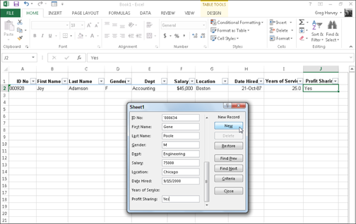
Figure 11-2: Enter the second record of the data list in its data form.

Whoa! Don’t press the Enter key to advance to the next field in a record. If you do, you’ll insert the new, incomplete record into the database.

Continue entering information for each field and pressing Tab to go to the next field in the database.

If you notice that you’ve made an error and want to edit an entry in a field you already passed, press Shift+Tab to return to that field.

To replace the entry, just start typing.

To edit some of the characters in the field, press → or click the I-beam pointer in the entry to locate the insertion point; then edit the entry from there.

When entering information in a particular field, you can copy the entry made in that field from the previous record by pressing Ctrl+’ (apostrophe). Press Ctrl+’, for example, to carry forward the same entry in the State field of each new record when entering a series of records for people who all live in the same state.

When entering dates in a date field, use a consistent date format that Excel knows. (For example, enter something like 7/21/98.) When entering zip codes that sometimes use leading zeros that you don’t want to disappear from the entry (such as zip code 00102), format the first field entry with the Special Zip Code number format (refer to Chapter 3 for details on sorting number formats). In the case of other numbers that use leading zeros, you can format it by using the Text format or put an ’ (apostrophe) before the first 0. The apostrophe tells Excel to treat the number like a text label but doesn’t show up in the database itself. (The only place you can see the apostrophe is on the Formula bar when the cell cursor is in the cell with the numeric entry.)

Press the key when you’ve entered all the information for the new record. Or, instead of the key, you can press Enter or click the New button (refer to Figure 11-2). Excel inserts the new record as the last record in the database in the worksheet and displays a new blank data form in which you can enter the next record (see Figure 11-3).

When you finish adding records to the database, press the Esc key or click the Close button at the bottom of the dialog box to close the data form.

Editing records in the data form

After the database is under way and you’re caught up with entering new records, you can start using the data form to perform routine maintenance on the database. For example, you can use the data form to locate a record you want to change and then make the edits to the particular fields. You can also use the data form to find a specific record you want to remove and then delete it from the database.

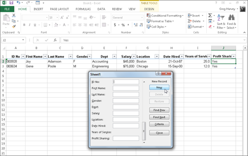
Figure 11-3: When you advance to a new record in the data form, Excel inserts the record just completed as the last row of the list.

Locate the record you want to edit in the database by bringing up its data form. See the following two sections (“Moving through records in the data form” and “Finding records with the data form”) and Table 11-1 for hints on locating records.

To edit the fields of the current record, move to that field by pressing Tab or Shift+Tab and replace the entry by typing a new one.

Alternatively, press ← or → or click the I-beam cursor to reposition the insertion point, and then make your edits.

To clear a field entirely, select it and then press the Delete key.

To delete the entire record from the database, click the Delete button in the data form. Excel displays an alert box with the following dire warning:

Displayed record will be permanently deleted

To delete the record displayed in the data form, click OK. To play it safe and keep the record intact, click the Cancel button.

You cannot use the Undo feature to bring back a record you removed with the Delete button! Excel is definitely not kidding when it warns permanently deleted. As a precaution, always save a back-up version of the worksheet with the database before you start removing old records.

Moving through records in the data form

In the data form, you can use the scroll bar to the right of the list of field names or various keystrokes (both summarized in Table 11-1) to move through the records in the database until you find the one you want to edit or delete.

To move to the data form for the next record in the data list: Press , press Enter, or click the down scroll arrow at the bottom of the scroll bar.

To move to the data form for the previous record in the data list: Press , press Shift+Enter, or click the up scroll arrow at the top of the scroll bar.

To move to the data form for the first record in the data list: Press Ctrl+, press Ctrl+PgUp, or drag the scroll box to the very top of the scroll bar.

To move to a new data form immediately following the last record in the database: Press Ctrl+, press Ctrl+PgDn, or drag the scroll box to the very bottom of the scroll bar.

Table 11-1 Ways to Get to a Particular Record

Keystrokes or Scroll Bar Technique	Result
Press or Enter or click the down scroll arrow or the Find Next button	Moves to the next record in the data list and leaves the same field selected
Press or Shift+Enter or click the up scroll arrow or the Find Prev button	Moves to the previous record in the data list and leaves the same field selected
Press PgDn	Moves forward ten records in the data list
Press PgUp	Moves backward ten records in the data list
Press Ctrl+ or Ctrl+PgUp or drag the scroll box to the top of the scroll bar	Moves to the first record in the data list
Drag the scroll box to almost the bottom of the scroll bar	Moves to the last record in the data list

Finding records with the data form

In a large data list, trying to find a particular record by moving from record to record — or even moving ten records at a time with the scroll bar — can take all day. Rather than waste time trying to manually search for a record, you can use the Criteria button in the data form to look it up.

When you click the Criteria button, Excel clears all the field entries in the data form (and replaces the record number with the word Criteria) so that you can enter the criteria to search for in the blank text boxes.

For example, suppose that you need to edit Sherry Caulfield’s profit sharing status. Unfortunately, her paperwork doesn’t include her ID number. All you know is that she works in the Boston office and spells her last name with a C instead of a K.

To find her record, you can use the information you have to narrow the search to all the records where the last name begins with the letter C and the Location field contains Boston. To limit your search in this way, open the data form for the Employee Data database, click the Criteria button, and then type C* in the text box for the Last Name field. Also enter Boston in the text box for the Location field.

When you enter search criteria for records in the blank text boxes of the data form, you can use the ? (for single) and * (for multiple) wild-card characters.

Now click the Find Next button. Excel displays in the data form the first record in the database where the last name begins with the letter C and the Location field contains Boston. The first record in this data list that meets these criteria is for William Cobb. To find Sherry’s record, click the Find Next button again. Sherry Caulfield’s record then shows up. Having located Caulfield’s record, you can then edit her profit sharing status from No to Yes in the text box for the Profit Sharing field. When you click the Close button, Excel records her new profit sharing status in the data list.

When you use the Criteria button in the data form to find records, you can include the following operators in the search criteria you enter to locate a specific record in the database:

Operator	Meaning
=	Equal to
>	Greater than
>=	Greater than or equal to
<	Less than
<=	Less than or equal to
<>	Not equal to

For example, to display only those records where an employee’s salary is greater than or equal to $50,000, enter >=50000 in the text box for the Salary field and then click the Find Next button.

When specifying search criteria that fit a number of records, you may have to click the Find Next or Find Prev button several times to locate the record you want. If no record fits the search criteria you enter, the computer beeps at you when you click these buttons.

To change the search criteria, first clear the data form by clicking the Criteria button again and then clicking the Clear button.

To switch back to the current record without using the search criteria you enter, click the Form button. (This button replaces the Criteria button as soon as you click the Criteria button.)

Sorting Data Lists

Every data list you put together in Excel will have some kind of preferred order for maintaining and viewing the records. Depending on the list, you may want to see the records in alphabetical order by last name. In the case of a client data table, you may want to see the records arranged alphabetically by company name. In the case of the Employee Data list, the preferred order is in numerical order by the ID number assigned to each employee when he or she is hired.

When you initially enter records for a new data list, you no doubt enter them in either the preferred order or the order in which you retrieve their records. However you start out, as you will soon discover, you don’t have the option of adding subsequent records in that preferred order. Whenever you add a new record, Excel tacks that record onto the bottom of the database by adding a new row.

Suppose you originally enter all the records in a client data list in alphabetical order by company (from Acme Pet Supplies to Zastrow and Sons), and then you add the record for a new client: Pammy’s Pasta Palace. Excel puts the new record at the bottom of the barrel — in the last row right after Zastrow and Sons — instead of inserting it in its proper position, which is somewhere after Acme Pet Supplies but definitely well ahead of Zastrow and his wonderful boys!

This isn’t the only problem you can have with the original record order. Even if the records in the data list remain stable, the preferred order merely represents the order you use most of the time. What about those times when you need to see the records in another, special order?

For example, if you usually work with a client data list in numerical order by case number, you might instead need to see the records in alphabetical order by the client’s last name to quickly locate a client and look up his or her balance due in a printout. When using records to generate mailing labels for a mass mailing, you want the records in zip code order. When generating a report for your account representatives showing which clients are in whose territory, you need the records in alphabetical order by state and maybe even by city.

To have Excel correctly sort the records in a data list, you must specify which field’s values determine the new order of the records. (Such fields are technically known as the sorting keys in the parlance of the database enthusiast.) Further, you must specify what type of order you want to create using the information in these fields. Choose from two possible orders:

Ascending order: Text entries are placed in alphabetical order from A to Z, values are placed in numerical order from smallest to largest, and dates are placed in order from oldest to newest.

Descending order: This is the reverse of alphabetical order from Z to A, numerical order from largest to smallest, and dates from newest to oldest.

Sorting on a single field

When you need to sort the data list on only one particular field (such as the Record Number, Last Name, or Company field), you simply click that field’s AutoFilter button and then click the appropriate sort option on its drop-down list:

Sort A to Z or Sort Z to A in a text field

Sort Smallest to Largest or Sort Largest to Smallest in a number field

Sort Oldest to Newest or Sort Newest to Oldest in a date field

Excel then re-orders all the records in the data list in accordance with the new ascending or descending order in the selected field. If you find that you’ve sorted the list in error, simply click the Undo button on the Quick Access toolbar or press Ctrl+Z right away to return the list to its order before you selected one of these sort options.

Excel shows when a field has been used to sort the data list by adding an up or down arrow to its AutoFilter button. An arrow pointing up indicates that the ascending sort order was used and an arrow pointing down indicates that the descending sort order was used.

Sorting on multiple fields

You need to use more than one field in sorting when the first field you use contains duplicate values and you want a say in how the records with duplicates are arranged. (If you don’t specify another field to sort on, Excel just puts the records in the order in which you entered them.)

---

---

The best and most common example of when you need more than one field is when sorting a large database alphabetically by last name. Suppose that you have a database that contains several people with the last name Smith, Jones, or Zastrow (as is the case when you work at Zastrow and Sons). If you specify the Last Name field as the only field to sort on (using the default ascending order), all the duplicate Smiths, Joneses, and Zastrows are placed in the order in which their records were originally entered. To better sort these duplicates, you can specify the First Name field as the second field to sort on (again using the default ascending order), making the second field the tie-breaker, so that Ian Smith’s record precedes that of Sandra Smith, and Vladimir Zastrow’s record comes after that of Mikhail Zastrow.

To sort records in a data list on multiple fields, follow these steps:

1. Position the cell cursor in one of the cells in the data list table.

2. If the Home tab on the Ribbon is selected, click Custom Sort on the Sort & Filter button’s drop-down list (Alt+HSU). If the Data tab is selected, click the Sort command button.

Excel selects all the records of the database (without including the first row of field names) and opens the Sort dialog box, shown in Figure 11-4.

3. Click the name of the field you first want the records sorted by in the Sort By drop-down list.

If you want the records arranged in descending order, remember also to select the descending sort option (Z to A, Largest to Smallest, or Newest to Oldest) in the Order drop-down list to the right.

4. (Optional) If the first field contains duplicates and you want to specify how the records in this field are sorted, click the Add Level button to insert another sort level. Select a second field to sort on in the Then By drop-down list and select either the ascending or descending option in its Order drop-down list to its right.

5. (Optional) If necessary, repeat Step 4, adding as many additional sort levels as required.

6. Click OK or press Enter.

Excel closes the Sort dialog box and sorts the records in the data list using the sorting fields in the order of their levels in this dialog box. If you see that you sorted the database on the wrong fields or in the wrong order, click the Undo button on the Quick Access toolbar or press Ctrl+Z to restore the database records to their previous order.

Check out how I set up my search in the Sort dialog box in Figure 11-4. In the Employee Data List, I chose the Last Name field as the first field to sort on (Sort By) and the First Name field as the second field (Then By) — the second field sorts records with duplicate entries in the first field. I also chose to sort the records in the Employee Data List in alphabetical (A to Z) order by last name and then first name. See the Employee Data List right after sorting (in Figure 11-5). Note how the Edwards — Cindy and Jack — are now arranged in the proper first name/last name alphabetical order.

Figure 11-4: Set up to sort records alphabetically by last name and then first name.

---

---

Figure 11-5:The Employee Data List sorted in alphabetical order by last name and then by first name.

Filtering Data Lists

Excel’s Filter feature makes it a breeze to hide everything in a data list except the records you want to see. To filter the data list to just those records that contain a particular value, you then click the appropriate field’s AutoFilter button to display a drop-down list containing all the entries made in that field and select the one you want to use as a filter. Excel then displays only those records that contain the value you selected in that field. (All other records are hidden temporarily.)

If the column headings of your data list table don’t currently have filter drop-down buttons displayed in their cells after the field names, you can add them simply by clicking Home⇒Sort & Filter⇒Filter or pressing Alt+HSF.

For example, in Figure 11-6, I filtered the Employee Data List to display only those records in which the Location is either Boston or San Francisco by clicking the Location field’s AutoFilter button and then clicking the (Select All) check box to remove its check mark. I then clicked the Boston and San Francisco check boxes to add check marks to them before clicking OK. (It’s as simple as that.)

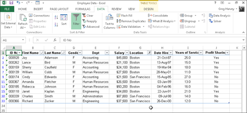
Figure 11-6: The Employee Data List after filtering out all records except those with Boston or San Francisco in the Location field.

After you filter a data list so that only the records you want to work with are displayed, you can copy those records to another part of the worksheet to the right of the database (or better yet, another worksheet in the workbook). Simply select the cells, then click the Copy button on the Home tab or press Ctrl+C, move the cell cursor to the first cell where the copied records are to appear, and then press Enter. After copying the filtered records, you can then redisplay all the records in the database or apply a slightly different filter.

If you find that filtering the data list by selecting a single value in a field drop-down list box gives you more records than you really want to contend with, you can further filter the database by selecting another value in a second field’s drop-down list. For example, suppose that you select Boston as the filter value in the Location field’s drop-down list and end up with hundreds of Boston records displayed in the worksheet. To reduce the number of Boston records to a more manageable number, you could then select a value (such as Human Resources) in the Dept field’s drop-down list to further filter the database and reduce the records you have to work with onscreen. When you finish working with the Boston Human Resources employee records, you can display another set by displaying the Dept field’s drop-down list again and changing the filter value from Human Resources to some other department, such as Accounting.

When you’re ready to display all the records in the database again, click the filtered field’s AutoFilter button (indicated by the appearance of a cone filter on its drop-down button) and then click the Clear Filter from (followed by the name of the field in parentheses) option near the middle of its drop-down list.

You can temporarily remove the AutoFilter buttons from the cells in the top row of the data list containing the field names and later redisplay them by clicking the Filter button on the Data tab or by pressing Alt+AT or Ctrl+Shift+L.

Using ready-made number filters

Excel contains a number filter option called Top 10. You can use this option on a number field to show only a certain number of records (like the ones with the ten highest or lowest values in that field or those in the ten highest or lowest percent in that field). To use the Top 10 option to filter a database, follow these steps:

1. Click the AutoFilter button on the numeric field you want to filter with the Top 10 option. Then highlight Number Filters in the drop-down list and click Top 10 on its submenu.

Excel opens the Top 10 AutoFilter dialog box. By default, the Top 10 AutoFilter chooses to show the top ten items in the selected field. However, you can change these default settings before filtering the database.

2. To show only the bottom ten records, change Top to Bottom in the left-most drop-down list box.

3. To show more or fewer than the top or bottom ten records, enter the new value in the middle text box (that currently holds 10) or select a new value by using the spinner buttons.

4. To show those records that fall into the Top 10 or Bottom 10 (or whatever) percent, change Items to Percent in the right-most drop-down list box.

5. Click OK or press Enter to filter the database by using your Top 10 settings.

In Figure 11-7, you can see the Employee Data List after using the Top 10 option (with all its default settings) to show only those records with salaries that are in the top ten. David Letterman would be proud!

Figure 11-7: The Employee Data List after using the Top 10 AutoFilter to filter out all records except for those with the ten highest salaries.

Using ready-made date filters

When filtering a data list by the entries in a date field, Excel makes available a variety of date filters that you can apply to the list. These ready-made filters include Tomorrow, Today, Yesterday, as well as Next, This, and Last for the Week, Month, Quarter, and Year. Additionally, Excel offers Year to Date and All Dates in the Period filters. When you select the All Dates in the Period filter, Excel enables you to choose between Quarter 1 through 4 or any of the twelve months, January through December, as the period to use in filtering the records.

To select any of these date filters, you click the date field’s AutoFilter button, then highlight Date Filters on the drop-down list and click the appropriate date filter option on the continuation menu(s).

Using custom filters

In addition to filtering a data list to records that contain a particular field entry (such as Newark as the City or CA as the State), you can create custom AutoFilters that enable you to filter the list to records that meet less-exacting criteria (such as last names starting with the letter M) or ranges of values (such as salaries between $25,000 and $75,000 a year).

To create a custom filter for a field, you click the field’s AutoFilter button and then highlight Text Filters, Number Filters, or Date Filters (depending on the type of field) on the drop-down list and then click the Custom Filter option at the bottom of the continuation list. When you select the Custom Filter option, Excel displays a Custom AutoFilter dialog box, similar to the one shown in Figure 11-8.

You can also open the Custom AutoFilter dialog box by clicking the initial operator (Equals, Does Not Equal, Greater Than, and so on) on the field’s Text Filters, Number Filters, or Date Filters submenus.

Figure 11-8: Use a custom AutoFilter to display records with entries in the Salary field between $25,000 and $75,000.

In this dialog box, you select the operator that you want to use in the first drop-down list box. (See Table 11-2 for operator names and what they locate.) Then enter the value (text or numbers) that should be met, exceeded, fallen below, or not found in the records of the database in the text box to the right.

Table 11-2 Operators Used in Custom AutoFilters

Operator	Example	What It Locates in the Database
Equals	Salary equals 35000	Records where the value in the Salary field is equal to $35,000
Does not equal	State does not equal NY	Records where the entry in the State field is not NY (New York)
Is greater than	Zip is greater than 42500	Records where the number in the Zip field comes after 42500
Is greater than or equal to	Zip is greater than or equal to 42500	Records where the number in the Zip field is equal to 42500 or comes after it
Is less than	Salary is less than 25000	Records where the value in the Salary field is less than $25,000 a year
Is less than or equal to	Salary is less than or equal to 25000	Records where the value in the Salary field is equal to $25,000 or less than $25,000
Begins with	Begins with d	Records with specified fields have entries that start with the letter d
Does not begin with	Does not begin with d	Records with specified fields have entries that do not start with the letter d
Ends with	Ends with ey	Records whose specified fields have entries that end with the letters ey
Does not end with	Does not end with ey	Records with specified fields have entries that do not end with the letters ey
Contains	Contains Harvey	Records with specified fields have entries that contain the name Harvey
Does not contain	Does not contain Harvey	Records with specified fields have entries that don’t contain the name Harvey

If you want to filter records in which only a particular field entry matches, exceeds, falls below, or simply is not the same as the one you enter in the text box, you then click OK or press Enter to apply this filter to the database. However, you can use the Custom AutoFilter dialog box to filter the database to records with field entries that fall within a range of values or meet either one of two criteria.

To set up a range of values, you select the “is greater than” or “is greater than or equal to” operator for the top operator and then enter or select the lowest (or first) value in the range. Then, make sure that the And option is selected, select “is less than” or “is less than or equal to” as the bottom operator, and enter the highest (or last) value in the range.

Check out Figures 11-8 and 11-9 to see how I filter the records in the Employee Data List so that only those records where Salary amounts are between $25,000 and $75,000 are displayed. As shown in Figure 11-8, you set up this range of values as the filter by selecting “is greater than or equal to” as the operator and 25,000 as the lower value of the range. Then, with the And option selected, you select “is less than or equal to” as the operator and 75,000 as the upper value of the range. The results of applying this filter to the Employee Data List are shown in Figure 11-9.

Figure 11-9: The Employee Data List after applying the custom AutoFilter.

To set up an either/or condition in the Custom AutoFilter dialog box, you normally choose between the “equals” and “does not equal” operators (whichever is appropriate) and then enter or select the first value that must be met or must not be equaled. Then you select the Or option and select whichever operator is appropriate and enter or select the second value that must be met or must not be equaled.

For example, if you want to filter the data list so that only records for the Accounting or Human Resources departments in the Employee Data List appear, you select “equals” as the first operator and then select or enter Accounting as the first entry. Next, you click the Or option, select “equals” as the second operator, and then select or enter Human Resources as the second entry. When you then filter the database by clicking OK or pressing Enter, Excel displays only those records with either Accounting or Human Resources as the entry in the Dept field.

Importing External Data

Excel 2013 makes it easy to import data into a worksheet from other database tables created with stand-alone database management systems (such as Microsoft Access), a process known as making an external data query.

You can also use web queries to import data directly from various web pages containing financial and other types of statistical data that you need to work with in the Excel worksheet.

Querying Access database tables

To make an external data query to an Access database table, you click the From Access command button on the Ribbon’s Data tab or press Alt+AFA. Excel opens the Select Data Source dialog box where you select the name of the Access database and then click Open. The Select Table dialog box appears from which you can select the data table that you want to import into the worksheet. After you select the data table and click OK in this dialog box, the Import Data dialog box appears.

The Import Data dialog box contains the following options:

Table to have the data in the Access data table imported into an Excel table in either the current or new worksheet — see Existing Worksheet and New Worksheet entries that follow

PivotTable Report to have the data in the Access data table imported into a new pivot table (see Chapter 9) that you can construct with the Access data

PivotChart to have the data in the Access data table imported into a new pivot table (see Chapter 9) with an embedded pivot chart that you can construct from the Access data

Only Create Connection to link to the data in the selected Access data table without bringing its data into the Excel worksheet

Existing Worksheet (default) to have the data in the Access data table imported into the current worksheet starting at the current cell address listed in the text box below

New Worksheet to have the data in the Access data table imported into a new sheet that’s added to the beginning of the workbook

Figure 11-10 shows you an Excel worksheet after importing the Invoices data table from the sample Northwind Access database as a new data table in Excel. After importing the data, you can then use the AutoFilter buttons attached to the various fields to sort and filter the data (as described earlier in this chapter).

Figure 11-10: Worksheet after importing an Access data table.

Excel keeps a list of all the external data queries you make so that you can reuse them to import updated data from another database or web page. To reuse a query, click the Existing Connections button on the Data tab (Alt+AX) to open the Existing Connections dialog box to access this list and then click the name of the query to repeat.

Databases created and maintained with Microsoft Access are not, of course, the only external data sources on which you can perform external data queries. To import data from other sources, you click the From Other Sources button on the Data tab or press Alt+AFO to open a drop-down menu with the following options:

From SQL Server to import data from an SQL Server table

From Analysis Services to import data from an SQL Server Analysis cube

From Windows Azure Marketplace to import data from any of the various marketplace service providers — note that you must provide the file location (usually a URL address) and your account key before you can import any marketplace data into Excel (visit www.windowsazure.com for details on using this service)

From OData Data Feed to import data from any database table following the Open Data Protocol (shortened to OData) — note that you must provide the file location (usually a URL address) and user ID and password to access the OData data feed before you can import any of its data into Excel

From XML Data Import to import data from an XML file that you open and map

From Data Connection Wizard to import data from a database table using the Data Connection Wizard and OLEDB (Object Linking and Embedding Database)

From Microsoft Query to import data from a database table using Microsoft Query and ODBC (Open Database Connectivity)

For specific help with importing data using these various sources, see my Excel 2013 All-In-One For Dummies.

Performing web queries

To make a web page query, you click the From Web command button on the Data tab of the Ribbon or press Alt+AFW. Excel then opens the New Web Query dialog box containing the Home page for your computer’s default web browser (Internet Explorer 10 in most cases). To select the web page containing the data you want to import into Excel, you can:

Type the URL web address in the Address text box at the top of the Home page in the New Web Query dialog box.

Use the Search feature offered on the Home page or its links to find the web page containing the data you wish to import.

When you have the web page containing the data you want to import displayed in the New Web Query dialog box, Excel indicates which tables of information you can import from the web page into the worksheet by adding a yellow box with an arrowhead pointing right. To import these tables, you simply click this box to add a check mark to it (see Figure 11-11).

Figure 11-11: Selecting the table of data to import on the Yahoo! Finance web page.

After you finish checking all the tables you want to import on the page, click the Import button to close the New Web Query dialog box. Excel then opens a version of the Import Data dialog box with only the Table option available where you can indicate where the table data is to be imported by selecting one of these options:

Existing Worksheet (default) to have the data in the Access data table imported into the current worksheet starting at the current cell address listed in the text box

New Worksheet to have the data in the Access data table imported into a new sheet that’s added to the beginning of the workbook

After you click OK in the Import Data dialog box, Excel closes the dialog box and then imports all the tables of data you selected on the web page into a new worksheet starting at cell A1 or in the existing worksheet starting at the cell whose address was entered in the text box in the Import Data dialog box.

Excel brings this data from the Volume Leaders table on the Yahoo! Finance web page into the worksheet as cell ranges rather than as an Excel Table. If you then want to be able to sort or filter this imported financial data, you need to select one of its cells and then select the Format as Table button on the Home tab to format them and add the requisite AutoFilter buttons (see Chapter 3 for details). When formatting data as a table, you remove all external connections to the data on the website.

You can make web queries only when your computer has Internet access. Therefore, if you’re using Excel 2013 on a portable device that can’t currently connect to the web, you won’t be able to perform a new web query until you’re in a place where you can connect.