8.4 CRM Implementation at a B2C Firm

A similar CLV management framework was also be implemented at a fashion retailer in a B2C setting. Like the IBM case study, this case study also highlights the power of the CLV metric and its related strategies in maximizing the retailer's profitability. This also showcases that CLV scores can be measured and effectively applied by the retailer to maximize both customer and store profitability. For instance, by performing segmentation, profile, and impact analysis in conjunction with the CLV score of the customers, retailers can uncover valuable customer-level insights thereby enabling them to deploy various customer management strategies. Similarly, CLV computation of customers by different stores can enable retailers to uncover some interesting and often counter-intuitive store-level insights leading to store management strategies.

8.4.1 The Focal Firm Background

The focal firm mentioned in this study is a fashion retailer, whose name is not revealed for confidentiality reasons. The retailer, which sells apparel, shoes, and accessories for both men and women, has a chain of 30 stores across the USA, with a relatively larger concentration of stores on the east and west coasts. Each of the stores was more or less of the same size and located in regions having similar demographics, thus there is no need to normalize the store's profit potential for these factors.

8.4.2 Implementing the CLV Management Framework at a Fashion Retailer

In essence, the key objective of the retailer was to maximize its profitability. Specifically, the study sought to answer the following research questions for the fashion retailer in particular and retailers in general [4]:

The customer data from the fashion retailer were utilized for this study. The total dataset comprised 303 431 customers after excluding 4% outliers from the original dataset that were consistently very high- or very low-value purchasers and probably would skew the sample's distribution. These 303 431 customers were then divided into two cohorts, as shown in Figure 8.5. Cohort 1, called ‘Model Building Sample,’ consisted of customers who made at least one purchase prior to December 31, 2003. Cohort 2, called ‘Model Validation Sample,’ consisted of customers who made at least one purchase prior to December 31, 2004 and who are not included in Cohort 1. Cohort 1 was used to calibrate the model and Cohort 2 was used to validate the calibrated model. There were 242 745 customers in Cohort 1 and 60 686 customers in Cohort 2.

The process adopted to develop the CLV-based framework for maximizing the retailer profits is illustrated in Figure 8.6. The idea was to use CLV as a basis for comparing the profit each customer brings to the firm. The aggregate profits all customers bring to a firm constitute its overall profit level. Therefore, to maximize the firm's overall profitability, the task was to implement marketing strategies that can maximize the profitability of each individual customer, or maximize the CLV score of each customer.

The framework provided in Figure 8.6 can be classified into three main stages: (1) model development, (2) model implementation, and (3) tactics and strategy recommendations. The following subsection reviews all these three stages and explains the process adopted in implementing this approach.

8.4.3 Process to Implement the CLV Management Framework at a Fashion Retailer

A clear picture of the process to implement the CLV management framework at the fashion retailer is provided in Figure 8.7. There are three main stages. In the first stage, just like the IBM case study, a CLV model was proposed and demonstrated as the most suitable model to measure future profitability for the retailer. In the second stage, based on the proposed CLV model, the CLVs of individual customers were measured, based on which the analyses of customers and stores were conducted. In the last stage, tactics and strategic recommendations were made based on the result of findings in the previous stages.

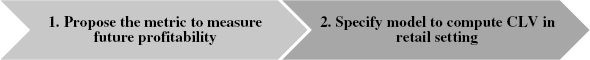
8.4.3.1 Stage 1: Model development

The model development stage involves two phases:

• Phase 1. Propose the metric to measure future profitability.
• Phase 2. Specify model to compute CLV in retail setting.

Phase 1: Propose the Metric to Measure Future Profitability

In this phase, the specific goals were to: (1) demonstrate the shortfall of traditional metrics, and (2) propose the CLV model as the more suitable model to measure the future profitability of a firm. The backward-looking characteristics of the traditional metrics were addressed, with specific reference to poor loyalty and profitability relationships shown by past research. Also, the forward-looking characteristic of the CLV metric was highlighted because it incorporated the future values/profitability that a customer can bring to a firm. Finally, the CLV metric was suggested as the superior metric to measure customer value and firm profitability.

Phase 2: Specify Model to Compute CLV in Retail Setting

In this phase, the desired output was the development of the CLV computation model. The always-a-share approach was adopted due to the non-contractual nature of the retailing sector. Based on this approach, a CLV model was formulated using discounted future value methodologies, which incorporated predictions of three key components, namely, purchase frequency, contribution margin, and marketing cost, as follows:

(8.10)

where:

GC_i,t = the gross contribution from customer i on purchase occasion t

c_i,m,l × x_i,m,l = the marketing cost (unit marketing cost × number of contacts) to customer i, in channel m, in time period l

frequency_i = the purchase frequency, computed as 12/expint_i because months are used as the units of analysis (expint_i is the expected interpurchase time for customer i)

r = discounted rate for money

n = number of years to forecast

T_i = total number of purchases made by customer i

i = index for customer

l = index for time period

t = index for time

m = index for channel

8.4.3.2 Stage 2: Model implementation

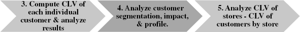
In this stage, the suggested CLV model was used to compute the actual CLV score of each individual customer, and conduct analyzes of the customers and stores, with the goal of maximizing the profitability of the retailer. Specifically, it involves the three following phases:

• Phase 3. Compute CLV of each individual customer and analyze results.
• Phase 4. Analyze customer segmentation, customer profile, and customer impact.
• Phase 5. Analyze stores – compute CLV of customers by store.

Phase 3: Compute CLV of Each Individual Customer and Analyze Results

This phase involved the prediction of the three main components of CLV model – purchase frequency, contribution margin, and marketing cost – by using the generalized gamma distribution, panel-data regression, and discounted future value methodologies respectively. Below is the detailed explanation of each step of this phase.

(a) Predicting the Purchase Frequency for Each Customer

To get the desired output, prediction of the purchase frequency for each customer, the purchase frequency was modeled using the likelihood function, generalized gamma distribution, and inverse generalized gamma distribution.

The Likelihood Function for Purchase Frequency Model

This model is given by

(8.11)

where:

f(t_ij | α, λ_i, γ) = the density function for the generalized gamma distribution, in other words the probability of the jth purchase for customer i occurring at time period t, given α, λ_i, γ.

S(t_ij | α, λ_i, γ) = the survival function for the generalized gamma distribution, in other words the probability of the jth purchase for customer i occurring at a time period greater than t, given α, λ_i, γ.

c_ij = the censoring indicator, where

c_ij = 1: if the jth interpurchase time for the ith customer is not right-censored

c_ij = 0: if the jth interpurchase time for the ith customer is right-censored

Φ_ijk = the probability of observation j for the ith customer belonging to subgroup k

α, λ_i, γ = the parameters of the generalized gamma distribution

The Expected Time until the Next Purchase Model

According to Equation 8.10, purchase frequency was computed as 12/expint_i because months were used as the units of analysis, where expint_i was expected interpurchase time for customer i, or the expected time until the next purchase. Given that the generalized gamma distribution was used to model the interpurchase time and the likelihood function in Equation 8.11, this expected time until the next purchase would be given by

(8.12)

where:

α, γ = the parameters that establish the shape of the interpurchase time distribution

λ_i = the individual specific purchase rate parameter, which in the generalized gamma distribution is assumed to be a random draw from an inverse generalized gamma distribution (IGG), specifically

where:

υ, γ = the shape and scale parameters of the IGG distribution respectively

γ = common parameters to both the generalized gamma distribution and the IGG distribution

k = the number of subgroups the population was assumed to consist of

Φ_ik = the probability of a customer belonging to each subgroup, and also provided the mass point (i.e., weight) for each subgroup. Φ_ik was modeled as a probit function of the antecedents and covariates of the purchase frequency. Specifically, the link function can be represented as , where x_ij are the antecedents and covariates of purchase frequency for customer i on purchase occasion j, and β_i are the customer-specific response coefficients.

The model framework presented in Equation 8.12 resembles a hierarchical Bayes formulation of the concomitant continuous mixture model. In order for the issue of endogeneity to be addressed, the one-period lagged value for all antecedents and covariates was used in the analysis [5, 6]. In addition, the performance of the proposed model framework was also evaluated with several alternative model formulations such as: (a) the simple generalized gamma distribution model, (b) the continuous mixture model, and (c) the latent class mixture model. Upon evaluation, the proposed model framework outperformed all the alternative model specifications. Finally, to account for any extraneous factors not accounted for by the antecedent and covariate set, the logarithm of the lagged interpurchase time was used. The specification of the model allowed the individual customer-level coefficients to be estimated for the influence of the various covariates on the probability of a customer belonging to a particular subgroup, hence the interpurchase times.

Results and Discussion of Findings

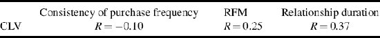
The finding showed a weak correlation between loyalty and observed future profitability. As given in Table 8.6, the correlation coefficients between observed future profitability and consistency of purchase frequency and RFM were both less than 0.3, while the correlation coefficient between observed future profitability (OFP) and relationship duration was the highest, 0.37. This result reinforced the argument that the retailer cannot afford to use traditional loyalty metrics to manage the customer relationship, which were backward looking. To manage both loyalty and profitability simultaneously, the retailer needed to adopt a forward-looking metric such as the CLV metric.

Table 8.6 Correlation of observed future profitability and different measures of loyalty.

(b) Predicting the Contribution Margin for each Customer

Gross Contribution Model

The gross contribution for each customer was modeled using the panel-data regression method. Gross contribution margin was defined as the revenue that the customer provides to the firm, whenever a purchase is made, minus the cost of goods sold. While the cost of goods sold does not change very much over time, the revenue a customer provides is likely to change over time. As a result, the gross contribution model was given by

(8.13)

where:

GC_ij = the gross contribution for customer i on purchase occasion j, measured in dollars

X_i,j−1 = the independent variable relevant to customer i on purchase occasion j − 1

e_i,j = the error term

n = the number of independent variables

k = the index for independent variables

i = the index for the customer

β₀, β_j = the coefficients

The performance of the proposed model framework, Equation 8.13, was evaluated with various alternative functional forms for gross contribution margin model, including (a) using log-margin as a dependent variable, and (b) a polynomial specification for the lagged dependent variables to allow for nonlinearity. The specification of Equation 8.13 provided the best in-sample fit and predictive accuracy. Any issues related to endogeneity were addressed by using lagged endogenous variables wherever necessary. The results were tested for multicollinearity using the variance inflation factor and eigenvalues of the principal component analysis of the predictors.

Results and Discussion of Findings

The result of the gross contribution model is provided in Table 8.7. This model provided a good model fit (R² = 0.71) and the mean absolute deviation (MAD) was 65 for the estimation sample and 70 for the holdout sample. The existence of a unit root in the gross contribution provided by a customer was rejected by the Dickey–Fuller test. On comparison, the proposed model outperformed the log-linear model. In addition, no significant nonlinear effects were observed for any of the parameters in the dataset.

Table 8.7 Results of the gross contribution model.

Variables	Standardized coefficients
Lagged contribution margins	0.83a
Lagged cumulative revenue from other channels	0.76a
Amount ($) spent on product category A on previous purchase occasion	0.61b
Time elapsed since last purchase	0.11a
Square of time elapsed since last purchase	−0.88b
a Significant at α = 0.01 level.
b Significant at α = 0.05 level.

Table 8.8 summarizes the results for the frequency model. The model had a log marginal likelihood (LMD) of 3.4 × 10⁴ and MAD = 2.4.

Table 8.8 Generalized gamma purchase frequency model.

Variables	Parameter estimates
Cross-purchase	6.9a
Number of distinct channels	6.1b
Number of returns	3.1a
Number of returns square	−1.7b
Log of lagged interpurchase time	−5.2a
a Posterior sample values between the 2.5th and 97.5th percentile do not contain zero.
b Posterior sample values between the 0.5th and 99.5th percentile do not contain zero.

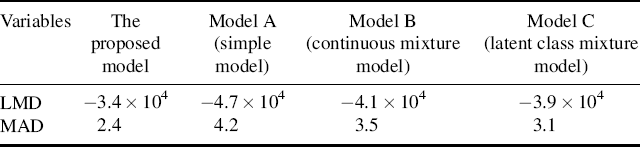
Table 8.9 provides a comparison of the performance of the above-proposed frequency model and alternative competing models described in earlier sections. As illustrated in Table 8.9, the proposed frequency model provided a better LMD and forecasting performance than the competing models. In essence, the concomitant mixture framework appears to be better suited to model abrupt changes in the interpurchase times, which was observed in the dataset.

Table 8.9 Comparison of proposed model with competing purchase frequency models.

(d) Predicting the Marketing Cost for each Customer

There are several ways to compute the marketing cost for each customer. For example, it may be calculated as an aggregate measure by dividing the total marketing budget by the number of customers. A more sophisticated approach would entail calculating the total marketing cost separately for each customer based on the various marketing channels expected to be used to interact with that customer. This approach to computing the marketing costs is given by

(8.14)

where:

MC_i = the total marketing cost for customer i

c_i,m,l = the unit marketing cost for customer i, in channel m, in time period l

m = the marketing channel (for this retailer it was the Web and catalog)

r = the discount rate

l = the index for time

n = the number of years to forecast

Equation 8.14 gives retailers the means to calculate the marketing cost not only on an individual customer basis, but also on the basis of individual marketing channels adopted for the same customer. This is very useful given the fact that direct marketing costs could vary widely across customers and across communication channels. For example, digital communications would cost much less than direct mailing. Furthermore, with the increasing trend of multi-channel marketing to the same customer, computing marketing costs as shown in Equation 8.14 can help retailers accurately arrive at a fair estimate of the expected marketing cost per customer. Accordingly, the expected marketing cost was discounted by l years to arrive at the present value of market cost.

For the purpose of computation, it was assumed that the direct marketing cost for each customer will be the same for the next three years. This assumption was applied because (1) the customer historical database shows that the historical direct marketing cost per customer remained more or less constant for the retailer, and (2) the retailer's directives were followed strictly. According to the retailer, the best prediction of future marketing cost of each customer over the next three years could be taken as three times the direct marketing cost in the most recent year (i.e., 2004). In this particular case study, the available marketing cost in the retailer's database was the total marketing cost (across all channels) for each customer.

After the three main components of the CLV model were predicted, Equation 8.10 was applied to calculate the CLV score of each individual customer.

Phase 4: Analyze Customer Segmentation, Customer Profile, and Customer Impact

The desired output of this phase was to answer the following questions:

• Which of the demographics, life style, and shopping behavior vary significantly across the high and low CLV segments?
• What is the impact of contribution margin and purchase frequency on high CLV segments of customers?

(a) Analyzing Customer Segmentation

Here, the CLV scores computed in Phase 3 were ranked in descending order and grouped into deciles so that each decile represents 10% of the customer base. Figure 8.8 shows the distribution of CLV scores across 10 deciles.

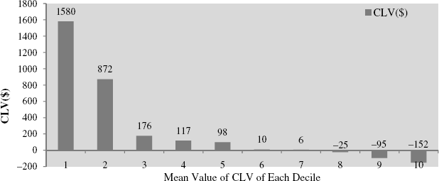
The result provided interesting insights. Most companies believe in the Pareto principle, or the 80:20 rule, which indicates that the top 20% (or 30%) of the customers typically generate 80% (or 70%) of the revenue or profits [7]. However, contrary to this belief, as shown in Figure 8.8 the top 20% (decile 1) were actually accounting for 95% of profits. This is because the bottom 30% had negative CLV.

Based on the above distribution of CLV scores, the entire customer group was divided into three segments: high CLV (comprising deciles 1 and 2), medium CLV (comprising deciles 3, 4, and 5) and low CLV segments (comprising deciles 6, 7, 8, 9, and 10). It should be noted that this form of segmentation is sensitive to the CLV scores of individual customers, thus the relative size of the segments will be subject to change over time if there are any changes to the CLV distribution.

(b) Analyzing Impacts of CLV Drivers on CLV Scores of Customers

In this section, the impact of CLV drivers on the three segments of high, medium, and low CLV was measured in the three following steps.

First, the key drivers of CLV (as outlined in Table 8.10) were selected to assess their impacts on CLV for the high CLV segment of customers. Second, the logistic regression method was used to determine which of these variables in the dataset (variables related to demographic, life style, and shopping behavior (DLSB)) varied significantly across the high and low CLV segments. In this case study, the medium CLV segment was excluded from the analysis to highlight the main difference between a high CLV and a low CLV customer. However, a similar procedure can be extended for medium CLV customers also if need be.

Table 8.10 Variables included for predicting purchase frequency and/or gross contribution.

The logistic regression method employed here is

(8.15)

where:

Prob_i = the probability of customer i to be in high or low CLV segment

Y_i = the outcome of regressing X_ik on high/low CLV segment indicator

X_ik = the ‘K’ DLSB (predictor) variables measured for customer i

β₀, β_k = the coefficients estimated from the data

This logistic regression method offered a simple procedure to estimate the coefficients by employing maximum likelihood.

Third, this model was run separately for the high and low CLV segments. In the model for the high CLV segment, the dependent variable was set as 1 if the customer belonged to the high CLV segment, or else 0. Similarly, in the model for the low CLV segment, the dependent variable was set as 1 if the customer belonged to the low CLV segment, or else 0. The findings from this analysis were then used to draw corresponding implications for customer profile analysis.

Finally, to assist the retailer's managers and develop strategies to increase the CLV of each customer, the impact of changing the values of some of the drivers of CLV in Table 8.10 was measured. High CLV customer segment and certain customer behavior-related variables were chosen for this measurement. Specifically, the magnitude of each driver was increased by 15% and the corresponding increase in CLV in each customer was evaluated. In practice, managers can make a similar impact on the value of each driver through appropriate marketing interventions, that is, promoting cross-buying behavior by offering customized incentives to customers to purchase across different product categories. The results presented in Figure 8.9 show that a 15% change in these key drivers significantly impacts the CLV of customers. These findings provide useful implications for customer and store management strategies.

(c) Analyzing Customer Profile

Based on the findings from the impact analysis, several group-level differences were identified. For instance, most high CLV customers were professionally employed and married females in the age range of 30–49 years old with at least one child, having high household income and the store's loyalty card. They also shopped in many channels and lived relatively close to the store. Low CLV customers, on the other hand, were primarily single men, in the age range of between 24 and 44 years old, having relatively low income and not necessarily the store's loyalty card. They shopped in one channel and lived further away from the retailer.

One advantage of this profile analysis is that it could help the retailer put a ‘face’ to the CLV score of the customer, which would give useful insights in acquiring new customers. This method also overcomes the shortcomings of most CLV studies, which do not include demographics and product usage variables [8].

Phase 5: Analyze CLV of Stores

The desired output of this phase was the CLV of a store. Customers of the retailer shop at several of the 30 store chains nationwide. Thus, it was possible to calculate the CLV of a store based on the CLVs of customers who have ever purchased from that store. This phase was divided into two smaller steps:

• To find the CLV score of customers by store.
• To find the CLV of a store.

The CLV score of customers by store was measured as the weighted average CLV of all customers shopping at that store. For example, suppose that customer 1 made 80% of his/her purchases from store A, 10% from store B, and 10% from store C. This information was used to assign customer value weights to each store. That is, store A can be assigned 80% of CLV from customer 1, 20% from customer 2, 0% from customer 3 (who did not shop at store A at all), and so on. The same procedure was then applied for all the stores.

The CLV of a store was measured as the weighted sum of the net present value of the CLVs of all customers that shop at that store minus the present value of the rent for the store. It should be noted that this method was based on the current set of customers, and did not take into account new customers that might be acquired by the store in the future.

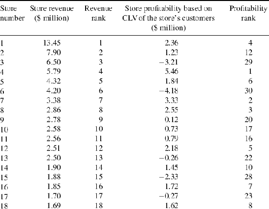
After all values of store CLVs were computed, all the stores were ranked according to both their past three-year profitability and future three-year profitability (store CLVs) (see Table 8.11). There was no need to normalize the stores' profit potential for the difference in size, location, and demographics, as they were more or less similar in terms of these factors. Finally, Spearman's correlation coefficients between the past and future profitability ranks were computed to draw corresponding implications for store management tactics and strategies.

Table 8.11 Comparison of store performance based on revenue and profitability.

8.4.3.3 Stage 3: Tactics and strategy recommendations

In this final stage, the result findings were used to suggest suitable tactics and strategy recommendations. The stage includes two phases:

• Phase 6. Customer management tactics and strategies.
• Phase 7. Store management tactics and strategies.

Phase 6: Customer Management Tactics and Strategies

The following managerial implications were suggested for the management of the retailer:

• Paradigm shift in management. The case study suggested that the CLV metric facilitated a paradigm shift in doing business by shifting the emphasis from managing customer relationship to managing customer value. This is because, while customer relationships are critical for all firms, they are just the means for the firms to achieve the overall goal of maximizing customer profitability. Managing customer value will directly have an impact on the firms' profitability.
• Customer value management. The result findings showed that as much as 30% of the retailer's customers had a negative CLV. Thus, it is important to obtain customer-level insights to design marketing strategies unique to each customer in order to maximize the value of the customer.
• Loyalty management. Given the weak relationship between the profitability and loyalty of customers, firms should adopt forward-looking metrics, such as the CLV metric, rather than backward-looking metrics in the management of both loyalty and profitability.
• Multi-channel shopping. The customer impact analysis revealed that a 15% increase in spending from other channels (e.g., through the Web and catalogs) by customers in the top two deciles leads to an 18% increase in their CLV scores. Therefore, it is advisable for the retailer to promote multi-channel shopping options to customers.
• Direct marketing. The customer profile analysis provided a clear snapshot of typical high and low CLV customer profiles. It also allowed the retailer to prioritize and target its sales and promotion campaigns effectively. For example, since the probability of finding less profitable customers, bargain hunters, is higher in the low CLV segment, the retailer should target its sales and promotional campaign to low CLV segments to avoid cannibalization of its business.
• Up-sell and cross-sell. Cross-purchase was a significant driver of the customer CLV that the retailer's managers should consider. In customer impact analysis, a 15% increase in cross-purchase of customers in the top two deciles resulted in the highest increase in their CLV, namely, 20%. Thus it was recommended that the retailer promote up-selling and cross-selling to customers that have low CLVs but have profiles similar to high CLV customers.
• Optimal resource allocation. Based on customer-level CLV score, the retailer was advised to set a ceiling on the dollar value for investing marketing resources in each customer to avoid overspending.

Phase 7: Store Management Tactics and Strategies

The retailer was advised to incorporate CLV metrics to store performance in order to increase its overall profitability. Two main management strategies were recommended:

• Identify the right customers for each store to target Based on customer profile analysis, managers should target or compare prospective customers to the high and low CLV customer profiles to make a decision on the right level of resources to acquire those customers.
• Determine the right marketing mix (4 Ps) to maximize the retailer's profitability. Recommendations were made for the following four strategies: pricing, promotion, location, and product, as follows. For the pricing strategy, the retailer should align price setting with the retailer's CLV structures, distribution, and characteristics, such as the price sensitivity of the high, medium and low CLV customers, the possibility of market cannibalization if the price for products typically purchased by high CLV customers was lowered, and so on. For the promotion strategy, the retailer was advised to align promotion with the retailer's profiles of the high, medium, and low CLV segments (such as responsiveness to in-store display and direct marketing, price sensitivities, special promotions, clearance sales, etc.). For the location strategy, since prime location might not translate into high profitability for a store, the retailer should evaluate a typical profile of high CLV customers and find a location that has a relatively high density of the targeted customers. For the product strategy, the retailer was advised to study the types of products that high, medium, and low CLV customer will buy, and target the right customer group accordingly. Importantly, it should ensure that a wide range of shopping options are available to customers.