4.6 SOW
Loyalty programs and direct mailings are two ways that companies use to manage customer relationships. The goal is to build close relationships with customers and thus enhance customers' relationship perceptions. Researchers have investigated the effects of companies' CRM efforts on customer retention and customer share development. Verhoef [4] considered customer retention as a binary outcome, and customer share of customer i for supplier j in category k at time t was defined as number of services purchased in category k at supplier j at time t divided by number of services purchased in category k from all suppliers at time t. The author first modeled customer retention with a probit model for all customers and then modeled customer share with a regression model for the customers who remained with the company. The author used Heckman's (1976) two-step procedure to correct for sample selection bias by incorporating the inverse Mills ratio obtained from the probit model. For both the probit and regression models, the author included past purchase behavior, customer relationship perceptions, and loyalty program dummy variables as independent variables. For the regression model, the difference between the logs of customer share at ![]() and
and ![]() was the dependent variable denoting the customer share development.
was the dependent variable denoting the customer share development.
Another important question related to repurchasing behavior and SOW was addressed by Leenheer et al. [26]. These authors investigated whether loyalty programs really do enhance behavioral loyalty (i.e., repeated purchase behavior). They also investigated the effect of these loyalty programs on a customer's SOW in a supermarket chain. Since the authors argued that the SOW a customer has for a store depends on its attraction to customers, the actual modeling task was to build an attraction model. In this case the SOW of a given customer was defined as
Since there were more than two stores in the study, the attraction to a store ![]() could not be modeled by binary logistic regression. Instead the authors chose to model the outcome using a multinomial logit model. This type of model is chosen when the dependent variable is nominal and has more than two categories. As an example, let us assume we have j categories and the first category is defined as the reference category. Then the log-odds ratio of the jth category is defined as
could not be modeled by binary logistic regression. Instead the authors chose to model the outcome using a multinomial logit model. This type of model is chosen when the dependent variable is nominal and has more than two categories. As an example, let us assume we have j categories and the first category is defined as the reference category. Then the log-odds ratio of the jth category is defined as
The predicted probability for categories ![]() relative to the reference category is
relative to the reference category is
and, for the reference category, the predicted probability is
Again, the multinomial logit model can be estimated by the MLE method. An introduction to the model from Greene's [27] econometric textbook is provided in Appendix appF. In Leenheer et al.'s (2007) study, the explanatory variables include household and store characteristics and loyalty program membership. These authors argued that an attraction model cannot take zeros but SOW can be zero if customers do not choose to buy from the store, so that in this case the authors used a probit model to estimate a selection variable to account for the correlated error terms of the attraction and SOW models. In addition, the authors argued that there might be a self-selection problem that loyal customers are more likely to enroll in a loyalty program leading to a potential endogeneity of loyalty program membership. To account for endogeneity, the authors adopted a two-stage least squares (2SLS) procedure using several instrumental variables to correct for the estimation bias of loyalty program membership.
In another study related to SOW, Cooil et al. (2007) used data from the Canadian banking industry to try and predict how changes in a customer's satisfaction would lead to changes in that customer's SOW at the given bank. These authors used a two-level latent class regression model to uncover the effect of changes in satisfaction on changes in SOW which were moderated by several demographic and situational characteristics. This two-level latent class regression was able to allow for household-level random effects within the latent class structure.
4.6.1 Empirical Example: SOW
Besides understanding a customer's purchase patterns from a given firm, many firms also want to understand how a customer spreads purchases in a given category across all firms. Research has shown that understanding a customer's SOW with a given firm can help understand the likelihood that a customer is going to repurchase from a given firm and inevitably the customer's long-term value to the firm. Thus, it can be useful to understand the drivers of SOW and in turn be able to predict each customer's expected SOW. At the end of this example we should be able to do the following:
The information we need for this model includes the following list of variables:
| Dependent variables | |
| Share-of-Wallet (SOW) | The percentage of purchases the customer makes from the given firm, given the total amount of purchases across all firms in that category |
| Independent variables | |
| Purchase_Rate | The average value for purchases across all 12 quarters |
| Avg_Order_Quantity | The average dollar value of the purchases in all 12 quarters |
| Avg_Crossbuy | The average value for cross-buy across all 12 quarters |
| Avg_Ret_Expense | Average dollars spent on marketing efforts to try and retain that customer in all 12 quarters |
| Avg_Ret_Expense_SQ | Square of average dollars spent on marketing efforts to try and retain that customer in all 12 quarters |
| Gender | 1 if the customer is male, 0 if the customer is female |
| Married | 1 if the customer is married, 0 if the customer is not married |
| Income | 1 if income < $30 000 |
| 2 if $30 001< income < $45 000 | |
| 3 if $45 001 < income < $60 000 | |
| 4 if $60 001 < income < $75 000 | |
| 5 if $75 001 < income < $90 000 | |
| 6 if income > $90 001 | |
| First_Purchase | The value of the first purchase made by the customer in quarter 1 |
| Loyalty | 1 if the customer is a member of the loyalty program, 0 if not |
In this case we have a limited dependent variable (SOW) which falls on the continuum between 1 and 100. The minimum is this case is 1% since all the customers in our database made at least one purchase with the given firm, and the maximum is 100% since all the customers in the database could potentially purchase these products from only this firm. Thus, we need to account for this bounded dependent variable. In this case we can use a variation of the Tobit model we used in previous examples. In the standard Tobit model case we have the situation where the lower bound of the dependent variable is defined, usually at 0, and the upper bound of the Tobit model is infinite. However, in this case we need to accommodate both the lower bound censoring and the upper bound censoring, where the lower bound is 1 and the upper bound is 100. Thus, we have the following definition for SOW:

In this case the SOW for customer i is only truly observed when the value is between 1 and 100. When the value of the SOW is 1 or 100, we only observe the censored value of SOW. To estimate this model we need to be able to handle observation-by-observation censoring using the following log-likelihood:

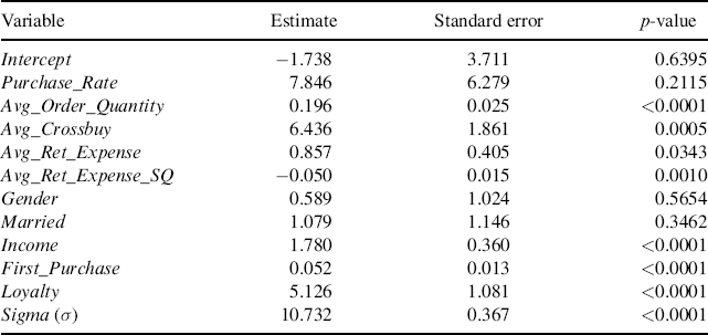
where SOW is the SOW of a given customer, X is the matrix of independent variables, β is the vector of coefficients of the independent variables, ϕ denotes the normal PDF, Φ denotes the normal CDF, and σ is the estimated standard error. Our objective then is to maximize the log-likelihood function through the estimation of the coefficients (β) and the standard error of the equation (σ). We get the following results when we estimate the model:

We gain the following insights from these results. We find that all the variables with the exception of Purchase_Rate, Gender, and Married are statistically significant at p < 0.05. We find that Avg_Order_Quantity is positive, suggesting that the higher the average past order values of the customer, the higher the SOW. We find that Avg_Crossbuy is positive, suggesting that the more a customer has bought across multiple categories in the past, the higher the customer's SOW. We find that Ret_Expense is positive with a diminishing return, as noted by the positive coefficient on Ret_Expense and the negative coefficient on Ret_Expense_SQ. This means that marketing efforts to retain and build relationships with the customer do cause the customer to have a higher SOW. Then, after the threshold is reached, marketing efforts actually decrease the SOW on average. This is likely due to the fact that overly contacting customers can often strain the relationship between the customer and firm. We find that three of the customer characteristic variables are positive (Income, First_Purchase, and Loyalty) suggesting that customers with a higher income, higher first-purchase value, and who are members of the loyalty program are likely to have a higher SOW.
Our next step is to predict the value of SOW to see how well our model compares to the actual values. We do this by starting with the equation for expected SOW. Given that we have a two-way censored model, we obtain the following equation:
![]()
where
![]()
In this case Φ is the normal CDF distribution, ϕ is the normal PDF distribution, Li is 1, Ri is 100, X is the matrix of independent variable values from the SOW equation, β is the vector of parameter estimates from the SOW equation, λ is the inverse Mills ratio, and σ is the standard error of the SOW equation. Once we have predicted SOW for each of the customers we want to compare this to the actual value from the database. We do this by computing the MAD. The equation is as follows:
![]()
We find for the acquired customers that MAD = 7.36, or on average 7.36% from the actual SOW. If we were to instead use the mean value of SOW (52.98) across all customers as our prediction for all customers (this would be the benchmark model case), we would find that MAD = 25.84, or on average 25.84% from the actual SOW. As we can see, our model does a significantly better job of predicting the value of SOW than the benchmark case.
4.6.2 How Do You Implement it?
In this example we used a two-sided censored regression to understand the drivers of SOW and predict SOW. Given the limited nature of the dependent variable we used PROC QLIM in SAS to estimate the model with a lower bound of 1 and an upper bound of 100. While we did use SAS to implement this modeling framework, programs such as MATLAB, R, and GAUSS can also be used.

