
Appendix J
Random Intercept Model
(Sources: Cameron and Trivedi [1], Hsiao [2])
The random effects model can be written as
or
where ![]() . The variance–covariance matrix of
. The variance–covariance matrix of ![]() is
is
Its inverse is
The individual-specific effects ![]() are assumed to be realizations of i.i.d. random variables with distribution
are assumed to be realizations of i.i.d. random variables with distribution ![]() and the error
and the error ![]() is i.i.d.
is i.i.d. ![]() . The model can be re-expressed as
. The model can be re-expressed as ![]() , where the error term
, where the error term ![]() has two components
has two components ![]() . For this reason the random effects model is also called the error components model or random intercept model. The random intercept model can be estimated by the maximum likelihood method.
. For this reason the random effects model is also called the error components model or random intercept model. The random intercept model can be estimated by the maximum likelihood method.
When ![]() and
and ![]() are random and normally distributed, the logarithm of the likelihood function is
are random and normally distributed, the logarithm of the likelihood function is
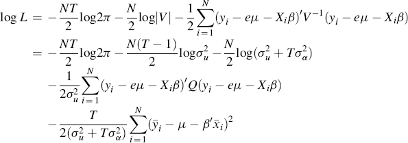
where
The maximum likelihood estimator (MLE) of ![]() is obtained by solving the following first-order conditions simultaneously:
is obtained by solving the following first-order conditions simultaneously:
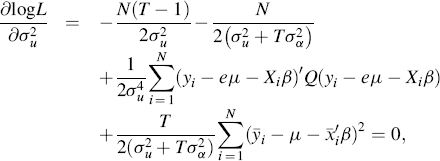

Simultaneous solution of Equations J.7–J.10 is complicated. The Newton–Raphson iterative procedure can be used to solve for the MLE. The procedure uses an initial trial value ![]() of
of ![]() to start the iteration by substituting it into the formula
to start the iteration by substituting it into the formula
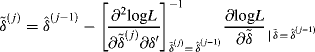
to obtain a revised estimate of ![]() . The process is repeated until the jth iterative solution
. The process is repeated until the jth iterative solution ![]() is close to the
is close to the ![]() th iterative solution
th iterative solution ![]() .
.