Simple spreadsheets are a good way to get a handle on Excel. But in the real world, you often need a spreadsheet that’s more sophisticated—one that can grow and change as you start to track more information. For example, on the expenses worksheet you created in Chapter 9, perhaps you’d like to add information about which stores you’ve been shopping in. Or maybe you’d like to swap the order in which your columns appear. To make changes like these, you need to add a few more skills to your Excel repertoire.
This chapter covers the basics of spreadsheet modification, including how to select cells, how to move data from one place to another, and how to change the structure of your worksheet. What you learn here will make you a master of spreadsheet manipulation.
First things first: before you can make any changes to an existing worksheet, you need to select the cells you want to modify. Happily, selecting cells in Excel—try saying that five times fast—is easy. You can do it many different ways, and it’s worth learning them all. Different selection techniques come in handy in different situations, and if you master all of them in conjunction with the formatting features described in Chapter 13, you’ll be able to transform the look of any worksheet in seconds.
Simplest of all is selecting a continuous range of cells. A continuous range is a block of cells that has the shape of a rectangle (high school math reminder: a square is a kind of rectangle), as shown in Figure 11-1. The easiest way to select a continuous range is to click the top-left cell you want to select. Then drag to the right (to select more columns) or down (to select more rows). As you go, Excel highlights the selected cells in blue. Once you’ve highlighted all the cells you want, release the mouse button. Now you can perform an action, like copying the cells’ contents, formatting the cells, or pasting new values into the selected cells.

Figure 11-1. Top: The three selected cells (A1, B1, and C1) cover the column titles. Bottom: This selection covers the nine cells that make up the rest of the worksheet. Notice that Excel doesn’t highlight the first cell you select.
In the simple expense worksheet from Chapter 9, for example, you could first select the cells in the top row and then apply bold formatting to make the column titles stand out. (Once you’ve selected the top three cells, press Ctrl+B, or chose Home → Font → Bold.)
Note
When you select some cells and then press an arrow key or click into another cell before you perform any action, Excel clears your selection.
Excel gives you a few useful shortcuts for making continuous range selections (some of these are illustrated in Figure 11-2):
Instead of clicking and dragging to select a range, you can use a two-step technique. First, click the top-left cell. Then hold down Shift and click the cell at the bottom-right corner of the area you want to select. Excel highlights all the cells in between automatically. This technique works even if both cells aren’t visible at the same time; just scroll to the second cell using the scroll bars, and make sure you don’t click any other cell on your way there.
If you want to select an entire column, click the header at the top of the column. For example, if you want to select the second column, then click the gray “B” box above the column. Excel selects all the cells in this column, right down to row 1,048,576.
If you want to select an entire row, click the numbered row header on the left edge of the row. For example, you can select the second row by clicking the gray “2” box to the left of the row. All the columns in this row will be selected.
If you want to select multiple adjacent columns, click the leftmost column header, and then drag to the right until all the columns you want are selected. As you drag, a tooltip appears indicating how many columns you’ve selected. For example, if you’ve selected three columns, you’ll see a tooltip with the text 3C (C stands for “column”).
If you want to select multiple adjacent rows, click the topmost row header and then drag down until all the rows you want are selected. As you drag, a tooltip appears indicating how many rows you’ve selected. For example, if you’ve selected two rows, you’ll see a tooltip with the text 2R (R stands for “row”).
If you want to select all the cells in the entire worksheet, click the blank gray box that’s just outside the top-left corner of the worksheet. This box is immediately to the left of the column headers and just above the row headers.

In some cases, you may want to select cells that are non-contiguous (also known as nonadjacent), which means they don’t form a neat rectangle. For example, you might want to select columns A and C, but not column B. Or, you might want to select a handful of cells scattered throughout the worksheet.
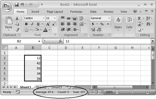
Figure 11-3. The nicest detail about the status bar’s quick calculations is that you can mix-and-match several at a time. Here, you see the count, average, and sum of the selected cells.
The trick to non-contiguous cell selection is using the Ctrl key. All you need to do is select the cells you want while holding down Ctrl. You can select individual cells by Ctrl-clicking them, or you can select multiple blocks of cells on different parts of the sheet by clicking and dragging in several different places while holding down Ctrl. You can also combine the Ctrl key with any of the shortcuts discussed earlier to select entire columns or rows as a part of your selection. Excel highlights in blue the cells you select (except for the last cell selected, which, as shown in Figure 11-4, isn’t highlighted because it becomes the active cell).

Figure 11-4. This figure shows a non-contiguous selection that includes four cells (A1, B2, C3, and B4). The last selected cell (B4) isn’t highlighted because it’s the active cell. This behavior is a little bit different from a continuous selection, in which the first selected cell is always the active cell. With a non-contiguous selection, the last selected cell becomes the active cell.
Excel provides a nifty shortcut that can help you select a series of cells without dragging or Shift-clicking anything. It’s called AutoSelect, and its special power is to select all the data values in a given row or column until it encounters an empty cell.
To use AutoSelect, follow these steps:
Move to the first cell that you want to select.
Before continuing, decide which direction you want to extend the selection.
Hold down Shift. Now, double-click whichever edge of the active cell corresponds to the direction you want to AutoSelect.
For example, if you want to select the cells below the active cell, then double-click its bottom edge. (You’ll know you’re in the right place when the mouse pointer changes to a four-way arrow.)
Excel completes your selection automatically.
AutoSelection selects every cell in the direction you choose until it reaches the first blank cell. The blank cell (and any cells beyond it) won’t be selected.
The mouse can be an intuitive way to navigate around a worksheet and select cells. It can also be a tremendous time-suck, especially for nimble-fingered typists who’ve grown fond of the keyboard shortcuts that let them speed through actions in other programs.
Fortunately, Excel is ready to let you use the keyboard to select cells in a worksheet. Just follow these steps:
Start by moving to the first cell you want to select.
Whichever cell you begin on becomes the anchor point from which your selected area grows. Think of this cell as the corner of a rectangle you’re about to draw.
Now, hold down Shift, and move to the right or left (to select columns) and down or up (to select more rows), using the arrow keys.
As you move, the selection grows. Instead of holding down Shift, you can also just press F8 once, which turns on extend mode. When extend mode is on, you’ll see the text Extend Selection in the status bar. As you move, Excel selects cells just as though you were holding down Shift. You can turn off extend mode by pressing F8 once you’ve finished marking your range.
Making a non-contiguous selection is almost as easy. The trick is you need to switch between extend mode and another mode called add mode. Just follow these steps:
Move to the first cell you want to select.
You can add cells to a non-contiguous range one at a time, or by adding multiple continuous ranges. Either way, you start with the first cell you want to select.
Press F8.
This key turns on extend mode. You’ll see the text Extend Selection appear in the Status bar to let you know extend mode is turned on.
If you want to select more than one cell, use the arrow keys to extend your selection.
If you just want to select the currently active cell, do nothing; you’re ready to go onto the next step. When you want to add a whole block of cells, you can mark out your selection now. Remember, at this point you’re still selecting a continuous range. In the steps that follow you can add several distinct continuous ranges to make a non-contiguous selection.
Press Shift+F8 to add the highlighted cells to your non-contiguous range.
When you hit Shift+F8, you switch to add mode, and you see the text “Add to Selection” appear in the status bar.
You now have two choices: You can repeat steps 1 to 4 to add more cells to your selection; or, you can perform an action with the current selection, like applying new formatting.
You can repeat steps 1 to 4 as many times as you need to add more groups of cells to your non-contiguous range. These new cells (either individuals or groups) don’t need to be near each other or in any way connected to the other cells you’ve selected. If you change your mind, and decide you don’t want to do anything with your selection after all, press F8 twice—once to move back into extend mode, and then again to return to normal mode. Now, the next time you press an arrow key, Excel releases the current selection.
Tip
You can also use the keyboard to activate AutoSelect. Just hold down the Shift key, and use one of the shortcut key combinations that automatically jumps over a range of cells. For example, when you hold down Shift and then press Ctrl+ →, you’ll automatically jump to the last occupied cell in the current row with all the cells in between selected. For more information about the shortcut keys, see Table 9-1 on Navigating in Excel.
One of the most common reasons to select groups of cells on a worksheet is to copy or move them from one place to another. Excel is a champion of the basic cut-and-paste feature, and it also gives you worthwhile enhancements that let you do things like drag-and-drop blocks of cells and copy multiple selections to the clipboard at the same time.
Before you get started shuffling data from one place to another, here are a few points to keep in mind:
Excel lets you cut or copy a single cell or a continuous range of cells. When you cut or copy a cell, everything goes with it, including the data and the current formatting.
When you paste cells onto your worksheet, you have two basic choices. You can paste the cells into a new, blank area of the worksheet, or, you can paste the cells in a place that already contains data. In this second case, Excel overwrites the existing cells with the new pasted data.
Cutting and copying cells works almost exactly the same way. The only difference you’ll see is that when you perform a cut-and-paste operation (as opposed to a copy-and-paste operation), Excel erases the source data once the operation’s complete. However, Excel doesn’t remove the source cells from the worksheet. Instead, it just leaves them empty. (The next section shows you what to do if you do want to remove or insert cells, not just the data they contain.)
Here’s the basic procedure for any cut-and-paste or copy-and-paste operation.
Select the cells you want to cut or copy.
You can use any of the tricks you learned in the previous section to highlight a continuous range of cells. (You can’t cut and paste non-contiguous selections.) When you want to cut or copy only a single cell, just move to the cell—you don’t actually need to select it.
If you want to cut your selection, choose Home → Clipboard → Cut (or Ctrl+X). When you want to copy your selection, choose Home → Clipboard → Copy (or Ctrl+C).
Excel highlights your selection with a marquee border (Figure 11-5), so-called because the border blinks like the twinkling lights around an old-style movie theater marquee.
Move to the new location in the spreadsheet where you want to paste the cells.
If you selected one cell, move to the new cell where you want to place the data. If you selected multiple cells, then move to the top-left corner of the area where you want to paste your selection. If you have existing data below or to the right of this cell, Excel overwrites it with the new content you’re pasting.
It’s valid to paste over part of the data you’re copying. For example, you could make a selection that consists of columns A, B, and C, and paste that selection starting at column B. In this case, the pasted data appears in columns B, C, and D, and Excel overwrites the original content in these columns (although the original content remains in column A).
Paste the data by selecting Home → Clipboard → Paste (or press Ctrl+V or Enter on the keyboard).
This action completes your cut-and-paste or copy-and-paste operation. When you’re performing a cut-and-paste, Excel removes the original data from the spreadsheet just before pasting it in the new location.

Tip
Instead of cutting or copying a block of cells, you can also move the entire column or row that contains the cells. Begin by highlighting one or more columns or rows (by selecting the column or row headers). For example, you could select column A by clicking the column header, and then cut it. You could then right-click the column B header, and choose Paste to move the column A values into column B. When you copy entire columns, Excel automatically adjusts the column widths as part of the copy operation, so the destination column winds up the same width as the source column.

If you want a really quick way to cut and paste data, you can use Excel’s drag-and-drop feature. It works like this:
Select the cells you want to move.
Just drag your pointer over the block of cells you want to select.
Click the border of the selection box, and don’t release the mouse button.
You’ll know that you’re in the right place when the mouse pointer changes to a four-way arrow. You can click any edge, but don’t click in the corner.
Drag the selection box to its new location. If you want to copy (rather than simply move) the text, hold down the Ctrl key while you drag.
As you drag, a light gray box shows you where Excel will paste the cells.
Release the mouse button to move the cells.
If you drop the cells into a region that overlaps with other data, Excel prompts you to make sure that you want to overwrite the existing cells. This convenience isn’t provided with ordinary cut-and-paste operations. (Excel uses it for drag-and-drop operations because it’s all too easy to inadvertently drop your cells in the wrong place, especially while you’re still getting used to this feature.)
In Windows’ early days, you could copy only a single piece of information at a time. If you copied two pieces of data, only the most recent item you copied would remain in the clipboard, a necessary way of life in the memory-starved computing days of yore. But nowadays, Excel boasts the ability to hold 24 separate cell selections in the Office clipboard. This information remains available as long as you have at least one Office application open.
Note
Even though the Office clipboard holds 24 pieces of information, you won’t be able to access all this information in Windows applications that aren’t part of the Office suite. If you want to paste Excel data into a non-Office application, you’ll be able to paste only the data that was added to the clipboard most recently.
When you use the Home → Clipboard → Paste command (or Ctrl+V), you’re using the ordinary Windows clipboard. That means you always paste the item most recently added to the clipboard. But if you fire up the Office clipboard, you can hold a lot more. Go to the Home → Clipboard section of the ribbon, and then click the dialog box launcher (the small arrow-in-a-square icon in the bottom-right corner) to open the Clipboard panel. Now Excel adds all the information you copy to both the Windows clipboard and the more capacious Office clipboard. Each item that you copy appears in the Clipboard panel (Figure 11-7).

Figure 11-7. The Clipboard panel shows a list of all the items you’ve copied to it since you opened it (up to a limit of 24 items). Each item shows the combined content for all the cells in the selection. For example, the first item in this list includes four cells: the Price column title followed by the three prices. If you’re using multiple Office applications at the same time, you may see scraps of Word documents, PowerPoint presentations, or pictures in the clipboard along with your Excel data. The icon next to the item always tells you which program the information came from.
Using the Clipboard panel, you can perform the following actions:
Click Paste All to paste all the selections into your worksheet. Excel pastes the first selection into the current cell, and then begins pasting the next selection starting in the first row underneath that, and so on. As with all paste operations, the pasted cells overwrite any existing content in your worksheet.
Click Delete All to remove all the selections from the clipboard. This is a useful approach if you want to add more data to the Clipboard, and you don’t want to confuse this information with whatever selection you previously copied.
Click a selection in the list to paste it into the current location in the worksheet.
Click the drop-down arrow at the right of a selection item to show a menu that allows you to paste that item or remove it from the clipboard.
Depending on your settings, the Clipboard panel may automatically spring into action. To configure this behavior, click the Options button at the bottom of the Clipboard panel to display a menu of options. These include:
Show Office Clipboard Automatically. If you turn on this option, the Clipboard panel automatically appears if you copy more than one piece of information to the clipboard. (Remember, without the Clipboard panel, you can access only the last piece of information you’ve copied.)
Show Office Clipboard When Ctrl+C Pressed Twice. If you turn on this option, the Clipboard panel appears if you press the Ctrl+C shortcut twice in a row, without doing anything else in between.
Collect Without Showing Office Clipboard. If you turn on this option, it overrides the previous two settings, ensuring that the Clipboard panel never appears automatically. You can still call up the Clipboard panel manually, of course.
Show Office Clipboard Icon on Taskbar. If you turn on this option, a clipboard icon appears in the system tray at the right of the taskbar. You can double-click this icon to show the Clipboard panel while working in any Office application. You can also right-click this icon to change clipboard settings or to tell the Office clipboard to stop collecting data.
Show Status Near Taskbar When Copying. If you turn on this option, you’ll see a tooltip near the Windows system tray whenever you copy data. (The system tray is the set of notification icons at the bottom-right corner of your screen, in the Windows taskbar.) The icon for the Office clipboard shows a clipboard icon, and it displays a message like “4 of 24 -Item Collected” (which indicates you have just copied a fourth item to the clipboard).
When you copy cells, everything comes along for the ride, including text, numbers, and formatting. For example, if you copy a column that has one cell filled with bold text and several other cells filled with dollar amounts (including the dollar sign), when you paste this column into its new location, the numbers will still have the dollar sign and the text will still have bold formatting. If you want to change this behavior, you can use the Paste Special command.
It works like this. First, copy your cells in the normal way. (Don’t cut them, or the Paste Special feature won’t work.) Then, move to where you want to paste the information, and choose Home → Clipboard → Paste → Paste Special (instead of Home → Clipboard → Paste). A new dialog box appears with a slew of options (Figure 11-8).
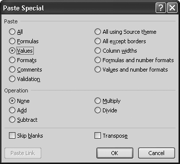
Figure 11-8. The Paste Special window allows you to choose exactly what Excel will paste, and it also lets you apply a few other settings. Here, Excel will paste the cell values but not the formatting.
These options are divided into two main groups: Paste and Operation. The Paste settings determine what content Excel pastes. This is the most useful part of the window. These settings include:
All. This option is the same as a normal paste operation, and it pastes both formatting and numbers.
Formulas. This option pastes only cell content—numbers, dates, and text— without any formatting. If your source range includes any formulas, Excel also copies the formulas.
Values. This option pastes only cell content—numbers, dates, and text—without any formatting. If your source range includes any formulas, Excel pastes the result of that formula (the calculated number) but not the actual formula.
Formats. This option applies the formatting from the source selection, but it doesn’t actually copy any data.
Comments. This option copies only the comments that you’ve added to cells.
Validation. This option copies only cells that use validation (an advanced tool for checking data before it’s entered into a cell).
All Except Borders. This option is the same as All, except it ignores any borders that you’ve applied to the cell. Border formatting is described on Borders and Fills.
Column Widths. This option is the same as All, and it also adjusts the columns in the paste region so that they have the same widths as the source columns.
Formulas and Number Formats. This option doesn’t paste any data. Here, Excel pastes only formulas and any settings used for formatting how numbers appear. (In other words, you’ll lose format settings that control the font, cell fill color, and borders.)
Values and Number Formats. This option pastes everything without any formatting, except for the formatting used to configure how numbers appear. (In other words, you’ll lose format settings that control the font, cell fill color, and borders.)
The Operation settings are a little wacky—they allow you to combine the cells you’re pasting with the contents of the cells you’re pasting into, either by adding, subtracting, multiplying, or dividing the two sets of numbers. It’s an intriguing idea, but few people use these settings because they’re not intuitive.
Further down the Paste Special dialog box, the "Skip blanks” checkbox tells Excel not to overwrite a cell if the cell you’re pasting from is empty. The Transpose checkbox inverts your information before it pastes it, so that all the columns become rows and the rows become columns. Figure 11-9 shows an example.

Figure 11-9. With the Transpose option (from the Paste Special dialog box), Excel’s pasted the table at the top and transposed it on the bottom.
Finally, you can use the Paste Link button to paste a link that refers to the original data instead of a duplicate copy of the content. That means that if you modify the source cells, Excel automatically modifies the copies. In fact, if you take a closer look at the copied cells in the formula bar, you’ll find that they don’t contain the actual data. Instead, they contain a formula that points to the source cell. For example, if you paste cell A2 as a link into cell B4, the cell B4 contains the reference =A2. You’ll learn more about cell references and formulas in Chapter 15.
Tip
Once you know your way around the different pasting options, you can often find a quicker way to get the same result. Instead of choosing Home → Clipboard → Paste → Paste Special, you can choose one of the options in the Home → Clipboard → Paste menu. You won’t find all the options that are in the Paste Special dialog box, but you do find commonly used options like Paste Values and Transpose.
Even if you don’t use the Paste Special command, you can still control some basic paste settings. After you paste any data in Excel, a paste icon appears near the bottom-right corner of the pasted region. (Excel nerds know this icon as a smart tag.) If you click this icon, you’ll see a drop-down menu that includes the most important options from the Paste Special dialog box, as shown in Figure 11-10.

Figure 11-10. The paste icon appears following the completion of every paste operation, letting you control a number of options, including whether the formatting matches the source or destination cells. If you choose Values and Number Formatting, Excel copies the cell content and the number formats, but ignores other formatting information like font and cell color. The number format determines how the number is displayed (for example, how many decimal places and whether a dollar sign is used). Chapter 13 covers formatting.
The cut-and-paste and copy-and-paste operations let you move data from one cell (or group of cells) to another. But what happens if you want to make some major changes to your worksheet itself? For example, imagine you have a spreadsheet with 10 filled columns (A to J) and you decide you want to add a new column between columns C and D. You could cut all the columns from D to J, and then paste them starting at E. That would solve the problem, and leave the C column free for your new data. But the actual task of selecting these columns can be a little awkward, and it only becomes more difficult as your spreadsheet grows in size.
A much easier option is to use two dedicated Excel commands designed for inserting new columns and rows into an existing spreadsheet. If you use these features, you won’t need to disturb your existing cells at all.
To insert a new column, follow these steps:
Select the column immediately to the right of where you want to place the new column.
That means that if you want to insert a new, blank column between columns A and B, start by selecting the existing column B. Remember, you select a column by clicking the column header.
Choose Home → Cells → Insert → Insert Sheet Columns.
Excel inserts a new column, and automatically moves all the columns to the right of column A (so column B becomes column C, column C becomes column D, and so on).
Inserting rows is just as easy as inserting new columns. Just follow these steps:
Select the row that’s immediately below where you want to place the new row.
That means that if you want to insert a new, blank row between rows 6 and 7, start by selecting the existing row 7. Remember, you select a row by clicking the row number header.
Choose Home → Cells → Insert → Insert Sheet Rows.
Excel inserts a new row, and all the rows beneath it are automatically moved down one row.
Note
In the unlikely event that you have data at the extreme right edge of the spreadsheet, in column XFD, Excel doesn’t let you insert a new column anywhere in the spreadsheet because the data would be pushed off into the region Beyond The Spreadsheet’s Edges. Similarly, if you have data in the very last row (row 1,048,576), Excel doesn’t let you insert more rows. If you do have data in either of these spots and try to insert a new column or row, Excel displays a warning message.
Usually, inserting entirely new rows and columns is the most straightforward way to change the structure of your spreadsheet. You can then cut and paste new information into the blank rows or columns. However, in some cases, you may simply want to insert cells into an existing row or column.
To do so, begin by copying or cutting a cell or group of cells, and then select the spot you want to paste into. Next, choose Home → Cells → Insert → Insert Copied Cells from the menu (or Home → Cells → Insert → Insert Cut Cells if you’re performing a cut instead of a copy operation). Unlike the cut-and-paste feature, when you insert cells, you won’t overwrite the existing data. Instead, Excel asks you whether the existing cells should be shifted down or to the right to make way for the new cells (as shown in Figure 11-11).
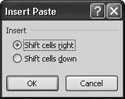
Figure 11-11. When you insert copied cells, Excel asks whether it should move the existing cells down or to the right.
You need to be careful when you use the Insert Copied Cells feature. Because you’re shifting only certain parts of your worksheet, it’s possible to mangle your data, splitting the information that should be in one row or one column into multiple rows or columns! Fortunately, you can always back out of a tight spot using Undo.
In Chapter 9, you learned that you can quickly remove cell values by moving to the cell and hitting the Delete key. You can also delete an entire range of values by selecting multiple cells, and then hitting the Delete key. Using this technique, you can quickly wipe out an entire row or column.
However, using delete simply clears the cell content. It doesn’t remove the cells or change the structure of your worksheet. If you want to simultaneously clear cell values and adjust the rest of your spreadsheet to fill in the gap, you need to use the Home → Cell → Delete command.
For example, if you select a column by clicking the column header, you can either clear all the cells (by pressing the Delete key), or remove the column by choosing Home → Cells → Delete. Deleting a column in this way is the reverse of inserting a column. All the columns to the right are automatically moved one column to the left to fill in the gap left by the column you removed. Thus, if you delete column B, column C becomes the new column B, column D becomes column C, and so on. If you take out row 3, row 4 moves up to fill the void, row 5 becomes row 4, and so on.
Usually, you’ll use Home → Cells → Delete to remove entire rows or columns. However, you can also use it just to remove specific cells in a column or row. In this case, Excel prompts you with a dialog box asking whether you want to fill in the gap by moving cells in the current column up, or by moving cells in the current row to the left. This feature is the reverse of the Insert Copied Cells feature, and you’ll need to take special care to make sure you don’t scramble the structure of your spreadsheet when you use this approach.