
Chapter 5
Sensitometry
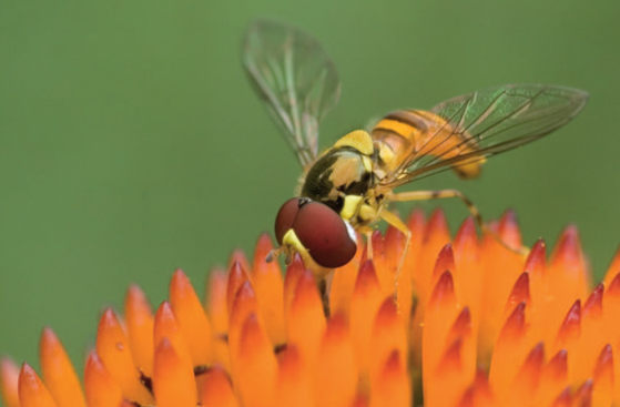
Photograph by Elliot Krasnopoler, Advertising Photography student, Rochester Institute of Technology
Introduction
Prior to the introduction of digital cameras, sensitometry was defined as the scientific evaluation of the response of a photographic emulsion to light. Today, sensitometry would better be defined as the scientific evaluation of a light-sensitive material to light. While there are some similar concepts between a digital system and photographic film sensitometric study, there are also many differences. The basic steps in a photographic film sensitometric study would be expose and develop the film, measure the densities, plot the data and analyze. The same process applies to doing a sensitometric study of photographic papers. For a digital sensitometric study, the process is to capture an image, determine the digital counts, plot the data and analyze, or instead of plotting data, the digital data can be analyzed using software.
Sensitometry provides quantitative information about light-sensitive materials. For a digital still camera (DSC), that would include such things as an ISO speed rating, recommended exposure index, and the standard output sensitivity. In a classic film-based system, these measurements would include an ISO speed rating, gamma value, contrast index, and exposure index.
Sensitometry can be further broken down into two main categories: camera and print. We will discuss the camera first for both digital and film systems. Prior to printing, photographers should have a complete understanding of how the image sensor or the film is performing. Once there is a complete understanding of the sensor or film, then a study of prints can take place.
Exposure
The exposure in both systems must be done in a controlled manner so that the input luminances are known. That is, we must be able to know what the subject input is. Several approaches can be used here.
The first approach would be to measure many different tones in an input scene. Areas of low lightness or reflectance would be shadow tones, while areas with high lightness are highlight tones. These reflected light values are luminances and are a measure of intensity of light per unit area. The basic unit of measurement is the candela per square foot.
Most photoelectric meters are equipped to measure the subject luminances by using the meter in the reflected light mode and pointing it at the area to be measured. The readings are usually in the form of arbitrary units that are proportional to the luminance in candelas per square foot.
An alternative method for obtaining input data about the subject is to use a reflection gray scale as a standardized reference. A gray scale is an organized set of subject tones displayed with known tonal values. These tonal values have been pre-measured on a reflection densitometer, and the values shown are reflection densities. Figure 5-1 shows two grayscales. Figure 5-1 (A) is commonly used for film studies and is inexpensive. Although it can also be used for digital cameras, the ISO has created a similar, more expensive target for use with digital cameras (see Figure 5-1(B)).
Most gray scales have a total luminance ratio of approximately 100:1 and are therefore close to representing an average outdoor scene that usually has a 160:1 luminance ratio. (A luminance ratio is the ratio of the brightest area in scene to the darkest area in the scene.) As input data, the only significant difference between grayscale data and subject log luminance values are that the numbers run opposite to each other. This is because reflection density is a measure of the amount of darkening occurring in an image, while luminance is a measure of the amount of light emanating from a surface. Therefore, the two concepts are reciprocally related. Although the concept of density will be addressed in detail later, it is important to note that the reflection densities of the gray scale are themselves logarithms, since, by definition, reflection density is the logarithm of the reciprocal of the reflectance.
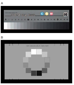
Figure 5-1 (A) Grayscale that can be used in tone reproduction studies. (B) ISO-14524 12-patch OECF target for use with digital cameras
When analyzing a digital system the accepted method for obtaining input data is to use the ISO 14524 target. The ISO has established a standard (ISO 12232) that outlines the required method for making an exposure when the resulting data will be used in a sensitometric study. The illumination should be either CIE illuminant D55 or tungsten illumination having a color temperature of 3,050 K. The ambient temperature of the area where the exposure is made should be (23 ± 2)° C with a relative humidity of (50 ± 20)%. The camera white balance should be adjusted so that the signal levels for the RGB are equal. That is, when the exposure is made, the white patch in the target should have equal values for the red, green, and blue digital counts. The IR blocking filter should be in place. In most cameras, this cannot be removed. The shutter speed shall not exceed 1/30 second. If possible, no compression will be done to the image prior to saving it on the camera memory card. All other camera setting options should be set to the manufacturer’s default settings. Finally, when making the exposure, the digital count values for the lightest patch on the target shall be as close to the maximum digital count available for the camera without clipping occurring.
For film, however, there is another option. Although cameras are the principal instruments used to expose film in practice, they are not the best choice for film testing purposes. The goal is for the film to receive a set of known exposures. The known illuminances and times are then used to calculate the exposures the film received. Because of light falloff and flare problems at the image plane, it is difficult to calculate accurate illuminance values from the subject luminances and the f-number. Additionally, the shutter speeds marked on most cameras may not correlate closely with the actual exposure times. Unless the shutter has been pre-tested and found to be consistent and accurate, reliable information about the exposure time will not be obtained. Devices specifically designed to expose film for testing purposes are called sensitometers.
Clipping is when a highlight region of a scene records at the largest pixel value available or a shadow region at the lowest pixel value.
A sensitometer consists of three major parts as shown in Figure 5-2: a light source, a step tablet, and a shutter. Sensitometers and cameras are both used to expose film. A sensitometer, however, has its own light source and subject (step tablet). Because a sensitometer is not a camera and is not a direct part of the picture-making process, great care is taken so it simulates actual picture-making conditions. For example, the light source is chosen so the color it produces matches that used in reality. Since the most commonly encountered light is daylight, sensitometric light sources that approximate its color quality are used. Usually, a tungsten lamp with appropriate filtration is used because it can be precisely calibrated and is very stable over its lifetime. Some sen-sitometers make use of a xenon-filled flashtube (electronic flash) source, which does not require filtration since its spectral output already is close to the color of daylight. Whatever source is used, the illumination reaching the film plane is nearly uniform and can be measured easily.
Sensitometers provide a systematic series of exposures for the purpose of studying the response of light sensitive materials.

Figure 5-2 The major parts of a sensitometer.
The step tablet serves as the subject for the sensitometer. It converts the single level of light produced by the lamp into many different levels or illuminances simulating the condition in the camera where the film receives varying illuminances due to the tonal differences in the scene.
An increase of 0.30 in density in a step tablet produces a decrease in exposure by the equivalent of one stop.
A step tablet is a series of calibrated filters with uniform density increments. Transmission density step tablets are available in a variety of sizes and formats. The most commonly used step tablet varies in density from approximately 0.10 to 3.10. When the step tablet is placed in the light path, the light is attenuated over a log range of 3.0 (3.10 - 0.10 = 3.00). Since densities are logarithmic values, the illuminances reaching the film plane will have a log range of 3.0. By taking the antilog of 3.0, we find that the ratio of illuminances will be 1000:1, which means that the highest illuminance is 1,000 times that of the lowest illuminance. With such a step tablet, the film will receive a ratio of illuminances far greater than that typically encountered in the camera, which is desirable for testing purposes.
If the tablet contains 11 different equally spaced steps, there will be 10 increments or intervals. Since the total density range is 3.0, the step-to-step difference can be determined by dividing 3.0 by 10, giving 0.30. This means that the steps get progressively denser in 0.30 increments. The antilog of 0.30 is 2, indicating a 2-times factor change in illuminance and exposure between successive steps (recalling that addition of logs corresponds to multiplication of antilogs). The step-to-step exposure change is equivalent to one stop, and the entire range covered is equal to 10 stops.
The shutter in a sensitometer performs the same task as the one in the camera: to control the length of time for which the light will strike the film. The shutter in a sensitometer usually is powered by a synchronous motor that operates in a repeatable fashion. A variety of exposure times can be achieved by using differing gear ratios and slit sizes. The actual exposure time should represent the times used in practice. Theoretically, any combination of illuminance and time giving equal numerical exposures could be used if the emulsion response depended only on the total amount of light received. Because the film responds differently to long and very short exposure times, an effect identified as reciprocity law failure (or reciprocity failure or reciprocity effect), an appropriate shutter speed must be selected to avoid the effect or an exposure adjustment will be needed. When the exposing source is a xenon flashtube, the flash duration governs the length of exposure time.
For the most part, photographers do not own or have access to sensitom-eters. Therefore, the use of a camera for sensitometry is often unavoidable. In this case, a reflection gray scale can be photographed and used as a test object. As seen earlier, reflection gray scales contain tonal values conveniently displayed from light to dark, and they are probably the most common test objects used in photography. Commercially available gray scales have a density range of approximately 2.0, which means a luminance ratio of 100:1 or about seven stops from the lightest to the darkest patch. The actual log values (reflection densities) are usually marked for each patch. If the gray scale has 10 different patches, then the film will receive 10 different exposures when the shutter is tripped.
This approach to sensitometry invariably leads to less precision in the resulting data for many reasons. First, when the gray scale is photographed, a nonlinear error is introduced as a result of optical flare in the camera, and there is a lack of image illuminance uniformity because of light falloff toward the corners. Further, the lighting of the original gray scale must be uniform and arranged to prevent reflections, including the subtle uniform reflections of light-colored walls or ceilings.
Sensitometers were developed for use with film, not with digital cameras. After all, it would be not be practical to remove the digital sensor from the camera to use it in a sensitome-ter. For the purposes of sensitometric studies in digital cameras, the use of a properly lit gray scale or the 12-patch OECF target as described previously is the approach most often used. The nonlinear error caused by light falloff of the lens and optical flare can be corrected digitally by photographing an 18% gray card under the same lighting conditions and normalizing the digital values of the gray-scale image with this data prior to printing. This effectively eliminates the problems that are encountered in a film system when this method is used.
Obtaining the proper exposure is key to successfully studying the tone reproduction of a digital camera. The exposure should place the brightest patch of the target at the highest digital count available without causing clipping in the system.
Digital Camera Sensitometry
After obtaining a properly exposed digital image and determining the exposures for each gray patch, there are many characteristics of the camera that can be examined. However, the first step in characterizing a digital camera is to plot the opto-electronic conversion function (OECF). The OECF illustrates how a digital camera converts the luminance at the sensor to digital counts. OECF is the relationship between the log luminance at the focal plane to the resulting digital counts. Log luminance (or also called log exposure) is plotted on the horizontal axis and digital count is plotted on the vertical axis. It would be analogous to a density versus log exposure curve (DLogH) for film, which will be discussed later.
The opto-electronic conversion function (OECF) is the digital equivalent of the density versus log exposure (DLogH) curve for film.
The OECF should start at a digital count of 0 and go to 255 if the camera outputs 8-bit data. For 12-bit data the range would be 0 to 4,095 and for 16-bit data the range would be 0 to 65,635. The OECF plot will have 3 lines on it, one each for the red, green, and blue layers.
Perhaps the simplest analysis to perform is to access the white balance of the camera. The white balance was set during exposure so that the white patch had equal digital count values for the R, G, and B layers. If the color balance algorithm is working properly, all three curves should plot directly on top of each other. In a digital system, to produce a neutral that does not have a color cast present in the image, the R, G, and B digital counts would have to be equal. This evaluation should be performed for all modes in which the camera will be used, including preset illuminants and manual white point setting.
The OECF is used to determine the camera’s dynamic range. The dynamic range can be thought of as the contrast of the scene. TO calculate the dynamic range, the lightest point on the OECF is found. This is the point where the illumination first produces the maximum output level for the camera. The darkest point is found at the illumination level where the signal-to-noise level passes the value of 3. The dynamic range is the contrast between these two points in contrast, f-stops, or densities.
The International Standards Organization (ISO) is a nonprofit organization that provides the standard procedure to calculate an ISO speed.
ISO Speed for Digital Cameras
The term ISO speed is familiar to all photographers. An ISO speed is a mathematical value that represents the sensitivity of a film or digital sensor to light. An ISO of 200 is twice as sensitive to light as ISO 100 and half as sensitive as an ISO of 400. An ISO’s most common use is with an exposure meter for determining the camera settings needed to achieve an acceptable image, negative, or transparency when being applied to film. ISO and exposure have a reciprocal relationship; the lower the ISO, the greater the exposure needed. The general relationship between speed and exposure is provided in Equation 5-1:
 (Eq. 5–1)
where H = the exposure in lux-sec-onds to achieve a certain result.
ISO speeds are determined for film and likewise for a digital camera. However, changing ISO speeds in these two systems means two very different things. For a film camera, it means changing to a different film that is more sensitive to light. In a digital camera, changing the ISO does not alter the sensitivity of the sensor. Changing the ISO amplifies the data coming from the sensor, effectively altering the gain of the electronic subsystem of the camera. However, this process amplifies both the image and the noise in the system.
In a digital system, there are two types of ISO ratings: saturation-based (ISO) and noise-based ISO. The saturation-based ISO is used when the photographer has control over the lighting levels such as in a studio. An exposure is selected that would place the highlight just short of the saturation level for the sensor. The noise-based ISO is appropriate when the lighting levels are less than ideal. In low-light situations, where exposures are longer or the ISO is higher, so is the noise level.
The ISO speeds present in a digital camera have been determined by the manufacturer according to ISO standard and are saturation-based speed values. To determine the saturation-based speed, the Equation 5-2 is used.
where Hsat is the minimum focal plane exposure that produces the maximum non-clipped camera output signal. The Ssat value is then found in Table 5-1 to locate the ISO speed.
The calculation of a noise-based ISO is a much more complicated procedure and is outlined in the ISO 12232:2006(E). To be performed accurately a programming environment such as MATLAB or ENVI’s IDL would be necessary. However, the Snoise values have been provided in Table 5-1 for comparison purposes.
Note that an ISO speed can only be determined when the standard is followed. However, that does not prevent photographers from calculating a speed for the conditions under which they are going to use the camera. The speed value would be accurate for those conditions, but could not be called an ISO speed.
Film Sensitometry
After the film has been exposed it must then be processed. This is an
Table 5-1 ISO speed, ISO speed latitude
| Ssat | Snoise | Reported Value |
| 8 <sat <10 | 10 <Snoise <12 | 10 |
| 10 <Ssat <12 | 12 <Snoise <16 | 12 |
| 12 <Ssat <16 | 16 <Snoise <20 | 16 |
| 16 <Ssat <20 | 20 <Snoise<25 | 20 |
| 20 <Ssat <25 | 25 <Snoise <32 | 25 |
| 25 <Ssat <32 | 32 <Snoise <40 | 32 |
| 32 <Ssat <40 | 40 <Snoise <50 | 40 |
| 40 <Ssat <50 | 50 <Snoise <64 | 50 |
| 50 <Ssat <64 | 64 <Snoise <80 | 64 |
| 64 <Ssat <80 | 80 <Snoise <100 | 80 |
| 80 <Ssat <100 | 100 <Snoise <125 | 100 |
| 100 <Ssat <125 | 125 <Snoise <160 | 125 |
| 125 <Ssat <160 | 160 <Snoise <200 | 160 |
| 160 <Ssat <200 | 200 <Snoise <250 | 200 |
| 200 <Ssat <250 | 250 <Snoise <320 | 250 |
| 250 <Ssat <320 | 320 <Snoise <400 | 320 |
| 320 <Ssat <400 | 400 <Snoise <500 | 400 |
| 400 <Ssat <500 | 500 <Snoise<640 | 500 |
| 500 <Ssat <640 | 640 <Snoise <800 | 640 |
| 640 <Ssat <800 | 800 <Snoise< 1000 | 800 |
| 800 <Ssat <1000 | 1000 <Snoise <1250 | 1000 |
| 1000 <Ssat <1250 | 1250 <Snoise <1600 | 1250 |
| 1250 <Ssat <1600 | 1600 <Snoise <2000 | 1600 |
| 1600 <Ssat <2000 | 2000 <Snoise <2500 | 2000 |
| 2000 <Ssat <2500 | 2500 <Snoise <3200 | 2500 |
| 2500 <Ssat <3200 | 3200 <Snoise <4000 | 3200 |
| 3200 <Ssat <4000 | 4000 <Snoise <5000 | 4000 |
| 4000 <Ssat <5000 | 5000 <Snoise <6400 | 5000 |
| 5000 <Ssat <6400 | 6400 <Snoise <8000 | 6400 |
| 6400 <Ssat <8000 | 8000 <Snoise <10000 | 8000 |
important step in the sensitometric process. When exposed film is developed, the latent image is amplified by as much as 10 million to 1 billion times. This tremendous amplification ability makes the silver halide system of photography so attractive, where even weak exposures can yield usable images. The result is a system with great sensitivity or, in the photographer’s vocabulary, a fast film.
The four major development factors are time, temperature, agitation, and developer composition.
There are four major factors in development—time, temperature, developer composition, and agitation. Agitation is the most difficult to standardize. The temperature of processing baths can be measured to an accuracy of ±1/10° F. The use of a reliable timer allows the length of development time to be controlled to within a few seconds. Prepackaged chemicals have reduced the problems involved in consistent developer composition. Proper agitation is difficult to achieve because, as we will see, there are at least two functions it must serve, and it must be different for different systems.
The laminar layer of used developer on the surface of film during development acts as a barrier to fresh developer.
One of the critical problems in the development of the latent image to metallic silver is obtaining uniform density in uniformly exposed large and small areas. Variations of density in uniformly exposed areas are usually damaging to image quality and are almost always due to non-uniform development. Proper agitation of the developing solution is the best safeguard of uniformity. Let us examine the effects of developing film with a total lack of agitation. Figure 5-3 illustrates such a stagnant tank condition. The sequence of events is as follows:
Correct agitation reduces uneven development.
1.e molecules of developer move around the tank in random fashion.
2.Since the concentration of developing agent is high in the developer and low in the emulsion, a transfer of the developing agent into the emulsion occurs. This transfer is called diffusion.
3.As the developing agent continues to diffuse into the emulsion it becomes attached to silver halide crystals.
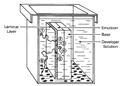
Figure 5-3 Stagnant tank (zero agitation) development. The numbers correspond to the sequence of events described in the text.
4.If the crystals have received an exposure to light, a chemical reaction occurs that produces metallic silver (the image) and developer reaction by-products.
5.The developer reaction by-products diffuse through and eventually out of the emulsion and into the developer solution.
6.Since some of these by-products are heavier than the developer solution, they tend to drift downward and collect on the bottom of the tank, creating an exhausted layer of developer.
Notice that the physical activity is completely based on the process of dif-fusion—diffusion of developing agents into the emulsion, and diffusion of development by-products out of the emulsion. Clearly, agitation can have nothing directly to do with this process of diffusion, a random molecular activity determined by the temperature and alkalinity of the developer, among other things.
We attempt to control the concentration of chemicals at the emulsion surface by agitation. There is always a relatively undisturbed thin layer of developer lying on the surface of the emulsion that is essentially stuck to the gelatin. This layer acts as a barrier, and as it becomes thicker, the process of diffusion is slowed. This explains why development times must be extended when little or no agitation is used during processing. Because this barrier or laminar layer is not the same thickness everywhere, it explains why improper agitation typically leads to uneven densities in uniformly exposed areas. In order for the barrier layer to be minimized, the fresh developer must make contact with the emulsion with a fair degree of force. Consequently, excellent agitation is characterized by vigorousness.
An additional function of agitation is to maintain the uniformity of the processing solution’s chemical composition and temperature. The agitation motions used should produce a random mix of both fresh and exhausted developer so that every part of the emulsion will have access to developer of the same composition. This is why it is generally not desirable to agitate film in a tray or tank in the same direction every time. The result of such nonrandom, directional movement is a lack of uniformity in the image.
There are many methods to agitate film while developing; in most cases, the typically used methods of tray, tank, and machine processing give acceptable results. However, when problems occur, most likely they are the result of deficiencies in one or both of these two characteristics: vigor and randomness.
Uniformity of development depends to a considerable extent on the degree or time of development. As the development time is increased and gamma infinity (maximum gamma) is approached, variations in time, temperature, and agitation have a decreased effect on image density and contrast. Thus it is more difficult to obtain uniform and consistent development of films that are developed to a low-con-trast index (as when photographing high-contrast scenes) than when developing to a higher-contrast index.
Transmittance, Density, Opacity
The most common method for determining the effect of exposure and processing on a sensitometric strip is to measure its light-stopping ability. This

Figure 5-4 Distribution of transmitted light rays caused by light scattering.
information provides excellent insight into the visual and printing characteristics of the image. When light strikes an image on the film, some of it is reflected backwards, some is absorbed by the black grains of silver, and some is scattered (that is, has its angle of travel changed) as a result of bouncing off grains. This is illustrated in Figure 5-4. The light-stopping ability of a silver photographic image is determined by a combination of these three optical occurrences. Notice that the light transmitted through the sample is distributed over a wide angle primarily as a result of the bouncing or scattering effect of the silver grains. For the moment, we will consider only the amount of transmitted light in relation to the amount of incident light on the sample.
Developing film to gamma infinity reduces the unevenness of development associated with poor agitation.
The formulas for Transmittance and Reflectance are similar:
T = transmitted light/incident light. R = reflected light/ incident light.
Basically, the transmittance (T) of a sample is the ratio of the transmitted light to the incident light as shown in Equation 5-3.
 (Eq. 5–3)
Consider, for example, the situation in Figure 5-5 where there are 100 units of light incident on the sample, and 50 units are transmitted. The transmittance would be (T) = 50/100, which is 0.50 or 1/2 or 50%. While this approach seems logical and direct, the
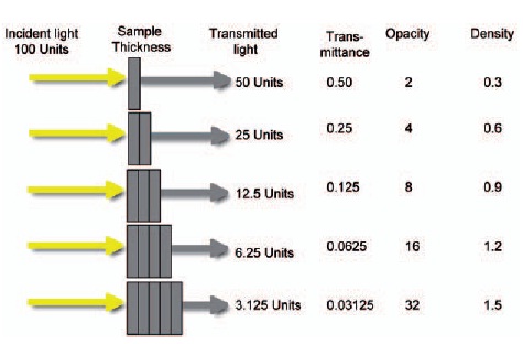
Figure 5-5 The relationship between sample thickness and transmittance, opacity and density.
disadvantage is that the transmittance, which describes a sample’s light-stopping ability, decreases as the light-stopping ability increases. For samples where the light-stopping ability is great, the transmittance is small.
Density equals the logarithm of the opacity or the logarithm of the reciprocal of the transmittance.
To overcome this shortcoming, we can calculate the opacity (O) of a sample, which is the ratio of incident light to transmitted light, and thus a reciprocal of the transmittance as shown in Equation 5-4. The formula is:
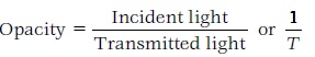 (Eq. 5–4)
In the example shown in Figure 5-5, the opacity (O) = 100/50, or 2. Opacity is the reciprocal of transmittance; as the sample’s light-stopping ability increases, so does the value for opacity, providing a more logical relationship. However, the potential awkwardness of opacity is revealed when considering the effects of equal increases in light-stopping ability.
Notice that as the thickness of the sample increases (and therefore, the light-stopping ability) in equal amounts by adding one sample atop another, the differences between the opacities are unequal as they become progressively greater. The opacities form a geometric (ratio) progression that becomes inconveniently large as the light-stopping ability increases. For example, ten thicknesses would give an opacity of 1,024.
To compensate for this problem, there is yet a third expression of the photographic effect called density. Density (D) is defined as the logarithm of the opacity (Eq. 5-5).
 (Eq. 5–5)
The density of the sample in Figure 5-5 is found as the log of 2, or 0.30.
Figure 5-5 illustrates the relationship of all three values, transmittance, opacity, and density. As the thickness of the sample increases, so do the density and the opacity. The transmittance has the reverse relationship, decreasing as transmittance increases.
The concept of density provides us with a numerical description of the image that is a more useful measure of light-stopping ability. An added benefit is that, as stated earlier, the visual system has a nearly logarithmic response, so our data will bear a relationship to the image’s appearance.
Density Measurement
Now that we have considered expressions of the image’s light-stopping ability, let us turn our attention to the practical problems of actually measuring the effect. Of the conditions of measurement, two are most important.
The first difficulty involves the measurement of the transmitted light. As shown in Figure 5-4, transmitted light rays form a distribution as a result of bouncing off the silver grains. This distribution of transmitted light will be wider for coarse-grained images than for fine-grained images because the larger grain size provides a greater surface area over which the bouncing can occur. Consequently, coarsegrained images scatter more light than fine-grained images.
Regardless of the grain size, the basic question is, where should the measurement of transmitted light be made? If, as shown in Figure 5-6, the receptor is placed far from the sample, only light transmitted over a very narrow angle will be recorded— this is called projection measurement. Alternatively, when the receptor is placed in contact with the sample, all the transmitted light will be collected, with the angle of collection being very large—this is referred to as a diffuse measurement. The projection density will be different from the diffuse density taken from the same sample.
For the companies that design and manufacture densitometers this difference between projection and diffuse density is a major concern, as it is for those who hope to apply their test results to a real picture-making situation. The answer lies in the principle that the testing conditions should simulate those used in practice. Therefore, if the negative is to be printed on a contact printer where the receptor (photographic paper) is in direct contact with the image, then the densitometer to be used should be similarly designed. For those negatives to be projection printed, the receptor will be far from the image, which indicates the opposite condition. These conditions represent extremes from very diffuse to very specular. Almost all commercially available densitometers are designed to provide an intermediate result termed a diffuse density.
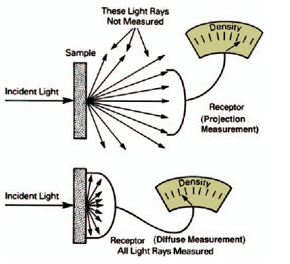
Figure 5-6 Two methods for measuring transmitted light.
It is important to realize that density measurements may come from an instrument that does not exactly simulate the particular photographic system being used. Trial-and-error is usually necessary to determine the appropriateness of the data. The relationship between the diffuse density and the projection density for a given sample may be determined and is called the Callier Coefficient or Q factor. See Equation 5-6.
Exposure meters and densitometers both measure light, but they express the measurements in different units.
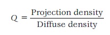 (Eq. 5-6)
The second problem associated with the actual conditions of density measurement is the color response of the densitometer. Photocells are typically used in densitometers to sense the light being transmitted. The color response characteristics of all photocells are not alike. Further, the color response of most photocells is unlike that of photographic printing papers. This would not be a significant problem if all the images being measured were perfectly neutral. However, we often measure negatives that are decidedly non-neutral as a result of using a fine-grain developer, a staining developer, or some after treatment of the negative. Indeed, when measuring the densities of color negatives, we never encounter neutral images.
Most commercial densitometers measure diffuse density, which is between projection density and doubly diffuse density.
At this point it is appropriate to ask—how will the densities be used? If the purpose is to predict the printing characteristics of a negative, the spectral response characteristics of the printing paper should be simulated. To determine the visual appearance of the image, the spectral response of the human eye should be simulated. In the first case, the result is called a printing density, in the second a visual density. These may be achieved by using certain filters in conjunction with the photocells. All commercially available densitometers are equipped to read visual density (sometimes referred to as black-and-white density). Only those specially equipped with the proper filters will read printing densities.
The color response of densitometers more closely matches the color response of the eye than that of black-and-white printing papers.
Characteristic Curves
Characteristic curves provide the relationship between the exposure (input from the subject) that the photographic film or paper received and the densities (the output image) that resulted. The equivalent in the digital environment is the opto-electronic conversion function (OECF) discussed earlier. The OECF provides the relationship between the exposure (input from the subject) that the sensor received and the digital count (the output image) that resulted.
In order to evaluate and understand the results of a sensitometric test, it is necessary to plot the densities occurring on the test strip in relation to the exposures that were received. The data contained in Table 5-2 illustrate the relationship between the input (exposure) data and output (density) data for a sensitometric test of a typical black-and-white negative film. It can be seen that each of the 11 densities produced is the result of a known exposure. The input data are given as both exposure and log exposure. When graphing the relationship, log exposure is used in preference to actual exposure to describe the input values because it tends to conveniently compress the input scale. The use of a logarithmic scale also makes it easier to determine exposure ratios, which are an important part of the evaluation process. Table 5-2 shows that exposures less than 1.0 lux-second are described by negative logarithms. Although the use of logarithms is addressed in Appendix C, it should be noted that negative logs are frequently encountered in sensi-tometry because the higher sensitivity of modern-day emulsions and digital sensors require only small amounts of exposure to yield image density or digital counts. Consequently, sensitometric exposures of less than 1.0 lux-second are common.
Notice in Table 5-2 that the differences in log exposure are 0.30 each, which is the result of using an 11-step tablet containing step-to-step density differences of 0.30. When plotting the data, actual log exposures or relative log exposures may be used as input data, depending upon what is known about the exposure conditions. The resulting graph will show log (or relative log) exposure on the horizontal axis as input and density on the vertical axis as output. Such a plot is referred to as a characteristic curve or D-log H curve. Older references call it the H&D curve after Hurter and Driffield, who first described the technique in the
Table 5-2 Relationship between exposure, log exposure, and the resulting density in a set of sensitometric exposures
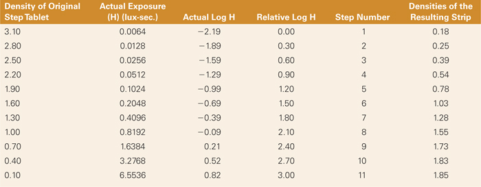
late 1800s, and later the D-log E curve. Figure 5-7 shows the curve resulting from a plot of the data in Table 5-2.
The curve in Figure 5-7 is typical of negative-working camera films. It can be conveniently divided into four major sections as follows:
1.Base plus fog.This is the area to the left of point A and is the combination of the density of the emulsion support (base) and the density arising from the development of some unexposed silver halide crystals (fog). Here the curve is horizontal and incapable of recording subject detail or tonal differences.
2.Joe. This is the section between points A and B and is characterized by low density and constantly increasing slope as exposure increases. Different subject tones will be reproduced as small density differences. It is in this area that shadow detail in the subject is normally placed.
3.Straight line. This portion, extending from point B to point C, is a middle-density region where the slope is nearly constant everywhere. It is also here that the slope of the curve is steepest—thus the subject tones are reproduced with the greatest separation (contrast). For many emulsions, however, the middle section of the curve is quite nonlinear, as will be seen later.
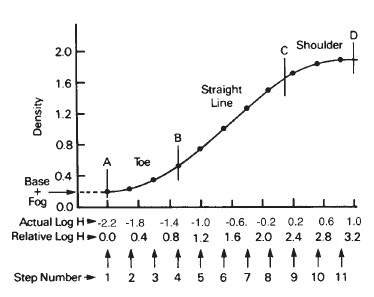
Figure 5-7 The characteristic curve resulting from the data in Table 4-2.
The pioneering work by Hurter and Driffield, reported in 1880, laid the foundation for sensitometry.
4.Shoulder. Located between points C and D, this is the portion where the density is high but the slope is decreasing with increases in exposure. Ultimately the slope approaches zero, where it is again impossible to record subject detail. Consequently, most of this section is usually avoided when exposing pictorial films.
A change in exposure of one stop, or a ratio of exposures of 1 to 2, corresponds to a change in log exposure of 0.3 on a characteristic curve.
The characteristic curve displays a “picture" of the film’s ability to respond to increasing amounts of exposure as a result of a specific set of development and image measurement conditions. It represents the single most commonly used method for illustrating the sensitometric properties of photographic materials and should be clearly understood.
Determining the Subject Luminance Range
The ability to determine the subject luminance range of a scene will allow the photographer to determine if a scene can be photographed without loss of detail in either the highlights or the shadows. Assume we are photographing the face of a model with highlight and shadow areas, illuminated so that the lighter side has eight times the luminance of the darker side, giving a subject-luminance ratio of 8:1. Since there are now two tones in the scene, there will be two image illuminances and, ultimately, two different exposures with one trip of the shutter. Figure 5-8(A) shows that these two input values will be separated by the log of 8, which is 0.90. If a second photograph is made of this subject, giving one stop more exposure, both log exposures will shift to the right a distance of 0.30 in logs but still will be separated by 0.90 because the subject luminances have not changed, as shown in Figure 5-8(B).
A one-stop change in camera exposure is the same as a 0.30 LogE change.
Therefore, the tones of the subject can be related to the log exposure axis of the characteristic curve. As shown above, the ratio of the subject
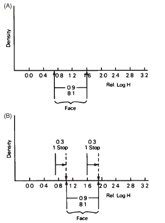
Figure 5-8 Changes in exposure for a simple two-tone scene as related to the log exposure axis.
luminances (highlights to shadows) plays a major part in determining the ratio of exposures (or range of log exposures) the film or sensor will receive. Also, by changing the camera settings or the level of light on the subject, the level of the exposures may be increased or decreased (shifted right or left) on the log exposure axis.
Exposure-Characteristic Curve Relationships
In reference to the simple two-tone scene described above, exposure and processing produced two different densities. The values of the two densities can be found by extending lines up from the two log exposure positions to the characteristic curve and then to the left until they intersect the density axis. This is illustrated in Figure 5-9A, which shows both log exposures falling on the straight-line section. The actual values of the densities are less important than the density difference because these relate to tonal separation or contrast. Therefore, density differences describe the amount of shadow, mid-tone, and highlight detail in the negative. In this example, the log exposures are separated by 0.90 (an exposure ratio of 8:1), while the resulting densities show a difference of only 0.60. This compression occurs because the slope of the straight-line section is less than 1.0 (45°). The actual slope may be computed by comparing the output density difference to the input log exposure difference. This leads to the generalized form for finding the slope (Eq. 5-7):
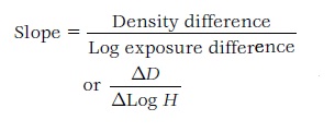 (Eq. 5-7)
For the situation shown in Figure 5-9(A) the AD is 0.60 and the Alog H is 0.90—and 0.60/0.90 is equal to 0.67, which is the slope of the straight-line region. This slope is related to the steepness of the curve and describes the rate at which density will increase as a result of increasing the exposure. A slope of 1.0 indicates that a change in log exposure will yield an equal change in density. With a slope of 0.50, the change in density is only half as great as the change in log exposure. The relationship can be restated as follows: Slope relates the negative contrast (density differences) to the subject contrast (log exposure difference). This relationship only applies to the straight-line section of the characteristic curve if indeed there is one.

Figure 5-9 Relationship between log exposure and density for two difference sections of the characteristic curve.
Where the section of the graph is a curve, as in the toe, there is no simple relationship between log exposure and density. Figure 5-9(B) shows the same two-toned scene placed entirely on the toe portion of the curve. In other words, the subject was given less exposure, as these log exposures are located to the left of the first. The resulting density difference is 0.20, which is considerably less than the first (0.60) because the slope in the toe is quite low. There will be far less tonal separation in this negative than in the first, that is, it has less contrast. If the slope were calculated as before, the resulting number would be related to an imaginary straight line drawn between the two density points and would not describe the actual slopes in the toe, which are everywhere different.
It should be clear that the contrast (density difference) of the negative is affected by changing the camera exposure. This will be the case either when there is no straight-line portion whatever or when the exposures are placed in a nonlinear area such as the toe and shoulder. If the subject tones are placed in the straight-line portion, they will be reproduced in the negative with the greatest possible separation (contrast). As the exposures become less and move into the toe region, the density differences of the shadows will rapidly decrease, and the shadow contrast will be reduced. If the exposures are increased and move into the shoulder region, the density differences of the highlights are quickly reduced, causing a loss of highlight contrast.
Total negative contrast, or TNC, is another name for negative density range.
In practice, the camera is likely to be aimed at scenes that range from about 20:1 to nearly 800:1, with 160:1 being average. Experience shows that excellent negatives are produced when the shadow exposures are placed in the toe of the curve, while the midtones and highlights fall in the midsection as shown inFigure 5-10. The shoulder section is almost always avoided because of the longer printing times required and the resulting loss of image quality. Most camera-speed pictorial films can accept these ranges and give excellent results.
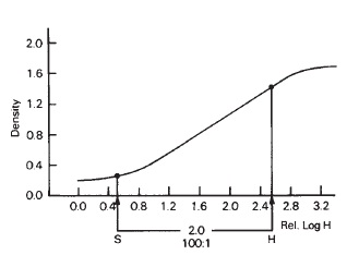
Figure 5-10 Proper placement of log exposures for an average-contrast scene.
Total negative contrast (the density difference between the thinnest and densest areas, also known as the density range) is largely determined by:
1.The subject contrast, which determines to a good first approximation the log H range on the horizontal axis of the D-log H curve.
2.The placement of this range of log exposures, determined by the camera settings.
3.The shape of the specific characteristic curve, which is mainly determined by the choice of emulsion and the development conditions.
The total negative contrast is a number similar in concept to the log of the subject luminance ratio. It describes the log range of output (that is, the density range) as a result of the previously mentioned conditions. For pictorial photographic negative emulsions, a total negative contrast of approximately 1.1 is considered normal (for diffusion enlargers) and is based on the printing characteristics of the negative. If the total negative contrast reaches 1.6, the negative is considered to have excessive contrast and probably is unprintable, even on a grade-one paper. When the total negative contrast is on the order of 0.4, it also will be nearly unprintable but because it is too flat for even a grade five printing paper.
Shadow detail, mid-tone contrast, and highlight detail are important, as noted earlier. A negative can have a large total negative contrast and still be totally lacking in shadow detail, as shown in Figure 5-11(A). Likewise, the total negative contrast may be great, but the highlights are blocked up, as in Figure 5-11 (B). Thus, we reach again the concept of slope as a measure of contrast in different parts of the film D-log H curve, and therefore in different parts of the negative (shadows, mid-tones, and highlights). A slope of 1.0 means the subject contrast is exactly duplicated in the negative. A lesser slope means the contrast is reduced, while a larger slope means it is increased. The correct contrast relationship is determined by the way the negative will be used and, in most cases, the way it will be printed, including the grade of paper that will be used. Interestingly, a normal-contrast negative actually has significantly less contrast than the original subject.
Log Exposure Range
In light of the relationship between subject luminances and camera exposures to the densities of the resulting negative, photographers should realize that excellent images can only be made if all the subject tones fall on the characteristic curve where there is sufficient slope. One of the most important measures of the sensitomet-ric properties of the film is the useful log exposure range. This is the range of log exposures over which the emulsion can produce adequate separation of densities and is based on the minimum slope required to achieve it. For example, as the camera exposure decreases, the subject tones move farther to the left into the toe and ultimately reach an area where the curve is completely flat (zero slope), resulting in a loss of detail in that portion—typically the shadows—of the negative. The smallest slope necessary to preserve acceptable shadow detail is located at a point on the toe that is the minimum useful point. Experiments using pictorial subjects indicate that the minimum useful point in the toe occurs where the slope is not less than 0.20, as illustrated in Figure 5-12(A).
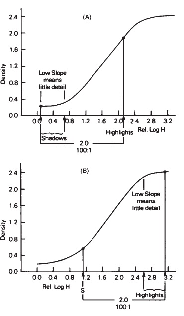
Figure 5-11 The relationship between slopes and density differences for underexposure and overexposure conditions with more than normal development.
Since the slope of a point cannot be found, the 0.20 refers to the slope of a line tangent to (just touching) the toe. For most camera-speed pictorial films this point of tangency usually falls at a density of not less than 0.10 above the base-plus-fog density and is referred to as the minimum useful density.
The location of the maximum useful point on the shoulder is known with less accuracy, partly because proper reproduction of the shadows is more important and partly because the highlight area of most scenes falls short of the shoulder portion.
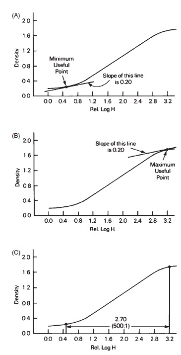
Figure 5-12 Determination of useful log exposure range. (A) Location of minimum useful point (shadows). (B) Location of maximum useful point (highlights). (C) Separation in logs along the horizontal axis (useful log exposure range).
However, experience indicates that the minimum useful slope on the shoulder is also approximately 0.20 and is found as shown in Figure 5-12(B). Since the shape of the upper portion of the curve highly depends upon the degree of development, no generalization can be made about the maximum useful density for the curve.
An average outdoor scene has a log exposure range of 2.20 and a luminance ratio of 160:1.
It is safer to overexpose negative film, black-and-white, and color, than to underexpose it.
Figure 5-12(C) illustrates the concept of useful log exposure range, which is the distance along the horizontal axis between the minimum and maximum useful points. In this example, the log range is 2.70, which means the useful exposure ratio is about 500:1 (antilog of 2.70 = 500). As long as the subject tones are placed between these points, the resulting negative will have acceptable detail in all areas. If the ratio of subject tones is so great that it exceeds the useful exposure ratio, either the shadows or the highlights will lack detail in the negative. Consequently, the useful log exposure range is a basic measure of the ability of a given film-developer combination to adequately record the subject tones.
Exposure Latitude
Associated with the useful log exposure range is the concept of exposure latitude, which relates to the margin for error in the camera exposure. For example, suppose we were using the film-developer combination resulting in the curve shown in Figure 5-12(C) to photograph a subject with a luminance ratio of 50:1. The subject will provide a log exposure range of 1.70 (log of 50 = 1.70). The useful log exposure range of the film-developer combination is 2.70, leaving a difference in logs of 1.00 (2.70 — 1.70 = 1.00). This means there is a 1.00 log interval left over that represents our margin for error. If the darkest shadow in the subject is to be placed at the minimum useful point as shown in Figure 5-13(A), the underexposure latitude is zero, while the overexposure latitude is 1.00 in logs, or a factor of 10, or 3 1/3 stops. When the lightest highlight is to be placed at the maximum useful point, the conditions are exactly reversed as illustrated in Figure 5-13(B). If the subject exposures are placed directly in the middle of the useful log exposure range as in Figure 5-13(C), the underexposure and overexposure latitude will be equal (1.00/2 = 0.50).
In practice, the shadows of the scene are usually placed at the minimum useful point because this allows for the highest effective film speed. The result is that exposure latitude in the camera is typically overexposure latitude only. Most camera-speed pictorial films have the capability of properly recording scenes with luminance ratios of up to 500:1. As the subject luminance ratio becomes greater, the exposure latitude becomes smaller, which creates a need for more accurate camera exposures. When the subject luminance ratios become excessive (greater than 500:1), special films and developers are required if excellent images are to be produced. The effect of camera flare light on image contrast will be considered later.
Effects of Development Time
Thus far we have considered only those properties that have been related to one curve and one development time. If a variety of development times are used with some less and some greater than the normal, a family of characteristic curves can be plotted as in Figure 5-14. Notice that all of the curves exhibit the same general shape. The following generalizations may be made:
1.Each curve shows a greater density in all areas as development time increases. Notice that base-plus-fog density is similarly affected.
2.The slope in the toe section is small and relatively unaffected by increases in development.

Figure 5-13 Exposure latitude: The relationship between subject log luminance range and the useful log exposure range. (A) Subject exposed for the darkest shadow allows overexposure. (B) Subject exposed for the lightest highlight allows underexposure latitude. (C) Subject placed in the middle of the useful log.
3.The slope of the midsection increases greatly as development time is increased.
4.The slope in the shoulder remains small for all development times, even though the density level changes dramatically.
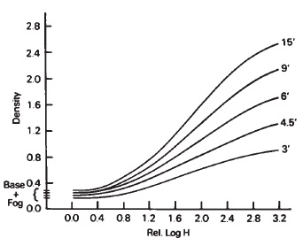
Figure 5-14 A family of curves for five different development times.
5.The useful log exposure range gradually becomes smaller as the development time increases, as a result of the higher slope of the straight line and a more prominent shoulder.
A common saying is to "Expose for the shadows and develop for the highlights."
Subject tones placed in the toe section of the curve will always be reproduced as small densities but, more significantly, with only slight separation of tone (contrast) regardless of the development time. When the subject tones are placed in the middle part of the curve, changes in development time will have a significant effect on the density differences produced. It is in the straight-line region where the photographer has the greatest control over contrast with development. Those subject tones placed in the shoulder section will result in high-density levels, but again with only little separation of tone for all development times.
Gamma = slope = AD/A Log H.
Since most pictorial photographic situations involve only the toe and midsection of the characteristic curve, it can be seen in practice that the darker tones (shadows) should govern camera exposure determination, while the lighter tones (highlights) should govern the degree of development. This idea is consistent with a common saying among photographers: Expose for the shadows and develop for the highlights. It should also be apparent that underexposure will shift the shadow tones farther to the left in the toe, where even lengthy development times will not produce a steep enough slope for the detail to be recorded. Further, the increase in development time will adversely affect the mid-tone and highlight reproduction by giving them unacceptably high contrast. This is typically the result when photographers attempt to push their film speed by underexposing and overdeveloping. This condition is illustrated in Figures 5-10 and 5-11 (A). Figure 5-10 shows the result of the proper placement of subject tones for a nearly average contrast scene with normal development. Figure 5-11 (A) shows the same scene but with the subject tones given less exposure, which places the shadow tones far into the toe region. The steeper slope of this curve is caused by an extended development time with the result being an obvious lack of shadow detail and excessive midtone and highlight contrast. The negative could well be unprintable on even the lowest contrast grade of paper.
Gamma
Of the several available measures of the contrast of photographic materials, gamma has the longest record of use. Gamma (y) is defined as the slope of the straight-line section of the D-log H curve as shown in Equation 5-8. The formula is as follows:
 (Eq. 5-8)

Figure 5-15 The determination of gamma for two different film samples.
where ΔD = the density difference between any two points on the straight-line portion of the curve, and ALog H = the log exposure difference between the two points chosen.
Examples of the determination of gamma are shown in Figure 5-15(A) and (B) for two different development times. Gamma is an excellent measure of development contrast because it is the slope of the straight-line portion that is most sensitive to development changes. It can also be used to predict the density differences that will result in the negative for exposures that fall on the straight-line section
If the gammas of all of the curves in Figure 5-14 are measured and plotted against the time of development, the curve shown in Figure 5-16 results. This is referred to as a time-gamma chart and illustrates the relationship between the slope of the straight line and the development conditions. For short development times, the gamma changes very rapidly, and as the time of development lengthens, the gamma increases more gradually. At some point in time, the maximum gamma of which this film-development combination is capable will be reached. This point is labeled gamma infinity and appears to be about 1.10 for these data. Since for this developer gamma increases greatly during short development times, extra care must be taken to minimize processing variability if consistent results are to be achieved. However, if longer times are used, the amount of development time latitude (margin for error in developing time) increases.
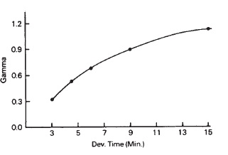
Figure 5-16 Development time vs. gamma chart for family of curves in Figure 5-14.
It is important to note here that gamma and negative contrast are different concepts. Gamma refers to the amount of development an emulsion receives, while negative contrast is concerned with density differences. Developing to a large gamma does not necessarily mean that a contrasty negative will result. The reason for this is that many factors in the photographic process affect the contrast of the negative, including the subject’s range of tones and the placement of the exposures on the D-log H curve.
Gamma is a measure of development contrast, which is only one of multiple factors that determine negative contrast.
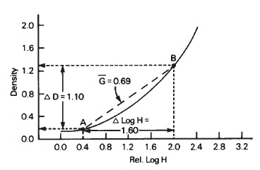
Figure 5-17 Determination of average gradient between two points on the curve.
Contrast index is the average slope of the most useful part of the film characteristic curve.
Average Gradient
In many cases, photographic materials do not provide a straight midsection, and in others there may be two straight-line sections with different slopes. Clearly, a single measure of gamma has little significance for these materials. Even for films exhibiting a single straight line, the useful portion of the curve usually includes part of the toe in addition to the straight line. In these situations where gamma cannot be used as a measure of slope, the concept of average gradient is substituted. An average gradient (G) is basically the slope of an artificial straight line connecting any two points on the curve, as illustrated in Figure 5-17. The D-log H curve shown here has no straight-line section, but the average gradient can be computed for the artificial line connecting points A and B by using the basic slope formula where slope = AD/Alog H. For this example, then: AD = 1.10, Alog H = 1.60,1 therefore:
The resulting number is a measure of the average contrast over the specified portion of the curve. Notice that this method can produce a variety of slopes by using different sections of the curve. Therefore, when interpreting average gradient data, be careful to note the section of the curve used.
Contrast Index
Another method for measuring the contrast of photographic emulsions is to determine the contrast index of the characteristic curve. Contrast index is an average gradient method with the added feature that the slope is always measured over the most useful portion of the curve. This approach evolved from an evaluation of the printing characteristics of a large number of excellent negatives made on a wide variety of emulsions. The result was a method for locating the most likely used minimum and maximum points on the curve and the determination of the average slope between them.
To determine the contrast index first, to locate a point on the toe that is 0.10 above base-plus-fog density. Using a compass, strike an arc with the center at this point and a radius of 2.0 in logs so that it intersects the upper portion of the curve. Then draw a straight line between these two points and determine its slope. The resulting number will be a close approximation of the contrast index.
In the manufacturer’s published data for a film, contrast index is used almost exclusively as a measure of development contrast. This is because contrast index is a measure of the slope over the area of the curve that will most likely be used when the negative is made. Therefore, unlike gamma, contrast index is an excellent measure of the relationship between the entire log exposure range of the subject and the entire density range of the negative, provided the subject has been exposed on the correct portion of the curve. This means that if the contrast index is 0.50, the total negative contrast (total density difference) will be just one-half the subject log exposure range. For example, an average outdoor scene has a luminance ratio of approximately 160:1 and will provide a log exposure range of nearly 2.20 (log of 160) to the film. A correctly exposed negative, processed to a contrast index of 0.50, will have a total negative contrast of 0.50 X 2.20 or 1.10, and will print easily on a normal grade of paper with a diffusion enlarger.
The important point here is that the required contrast index may be changed to suit the subject log luminance range. Thus if the scene is excessively contrasty, development to a low contrast index will generate a negative that will print on a normal grade of paper. On the other hand, if the scene is unusually flat, the film may be developed to a high contrast index to obtain a normal contrast negative.
ISO Film Speed
Sensitometry in a film system is the measurement of the emulsion sensitivity to light or, more commonly, the film speed. The concept of film speed and its relationship to the determination of the proper camera exposure should be clearly understood because, as we have seen, significant errors in the exposure of the film often cannot be rectified later.
Most pictorial negative films have film speed ratings computed by the manufacturer and published as ISO (ASA) values. This means that the speed has been determined in accordance with the procedures described by the American National Standards Institute (ANSI) and the ISO. Both organizations are nonprofit operations that exist for the purpose of providing standard procedures and practices to minimize variations in testing. Since there are many sources for variation in the determination of film speed, it is highly desirable to have an agreed-upon method that is accepted by a majority as the best technique. The ISO standard for film, just as for digital, provides guidelines for the type of exposing light (daylight), the exposure time (1 second to 1/1,000 second), the developer composition (a formula devised for testing purposes that is not commercially available), the type of agitation, and the amount of development (an average gradient of approximately 0.62) for preparing a film for a speed calculation. Once all these conditions have been met, the speed point is located at a density of 0.10 above base plus fog and the following formula is used:
 (Eq. 5-9)
where: Hm = the exposure in lux-seconds that gives a density of 0.10 above base plus fog, and 0.8 = a constant that introduces a safety factor of 1.2 into the resulting speed value. The film is actually 1.2 X faster than the published value, which guards against underexposure.
Film speeds are based on the amount of exposure that is required to produce a specified density.
ISO (ASA) speeds are rounded to the nearest third of a stop using the standard values listed in Table 5-3. Therefore, each ISO (ASA) speed value has a tolerance of ±1/6 stop. Consider the curve shown in Figure 5-18, which is the result of following the ISO (ASA) standard procedures. The determination of speed is as follows:
Table 5-3 ISO (ASA) and ISO (DIN) standard speed values
| ASA (Arithmetic) | DIN (Logarithmic) | ASA (Arithmetic) | DIN (Logarithmic) |
| 6 | 9° | 250 | 25° |
| 8 | 10° | 320 | 26° |
| 10 | 11° | 400 | 27° |
| 12 | 12° | 500 | 28° |
| 16 | 13° | 650 | 29° |
| 20 | 14° | 800 | 30° |
| 25 | 15° | 1000 | 31° |
| 32 | 16° | 1250 | 32° |
| 40 | 17° | 1600 | 33° |
| 50 | 18° | 2000 | 34° |
| 64 | 19° | 2500 | 35° |
| 80 | 20° | 3200 | 36° |
| 100 | 21 ° | 4000 | 37° |
| 125 | 22° | 5000 | 38° |
| 160 | 23° | 6400 | 39° |
| 200 | 24° |
ISO film speeds are rounded to the nearest one-third of a stop.

Figure 5-18 The determination of ISO (ASA) speed for a specific sample.
1.Locate point m at 0.10 above the base-plus-fog density, which in this case is at a gross density of 0.20.
2.Beginning at point m, move a distance of 1.30 in log units to the right along the log exposure axis.
3.From this position, move up a distance of 0.8 in density units, and if the curve crosses at this point (±0.05), the proper contrast has been achieved and the speed may be computed at point m. If not, the test must be rerun using a development time that yields the proper curve shape.
In this example, the curve shape is correct, and the log exposure at the speed point is -2.6. Taking the antilog of this value, the exposure is found to be 0.00251 lux-second. Substituting, we have:
Using the values in Table 5-3, the ISO (ASA) speed would be expressed as 320. The manufacturer’s published values for a given film type are determined by sampling many emulsion batches and averaging the test results.
Following the ISO standard results in film speeds that mean the same thing for all pictorial negative films regardless of the manufacturer. It also means that a given emulsion has only one ISO (ASA) speed, and this value cannot be changed as a result of using a special developer because the conditions of testing have been specified. Any change in these conditions means the standard has not been followed, and, therefore, by definition the ISO (ASA) speed cannot be found. In practice, most photographers will necessarily use conditions different from those outlined in the standard. For example, if tungsten light is used or a special-purpose developer tried, the circumstances of practice no longer match those of the test. This is an unavoidable pitfall of the ISO (ASA) published speeds—once the best method has been agreed upon and standardized, the speeds are only valid for those conditions. It is common for film manufacturers to publish both daylight and tungsten speeds for some non-pan-chromatic emulsions.
Analysis of Negative Curves
When surveying the wide variety of black-and-white negative working emulsions available, it becomes an imposing task to describe the properties of each. Fortunately, this diverse collection of emulsions can be organized on the basis of contrast (as seen in the curve shape) and film speed. Although there are other considerations for the grouping of films, such as format and image structure, it seems appropriate at this point to consider the sensitometric properties, as they have the greatest influence upon the intended use of the emulsion. Negative-working films can be categorized as normal-contrast films, continuous-tone copy films, or line-copy films.
Normal-contrast films are intended to be used with pictorial subjects with the final product being a reflection print. They will have a contrast index of approximately 0.60 when developed normally. The ISO of these films will typically range from 32 to 4000.
Separate daylight and tungsten film speeds are published for some films.
The characteristic curves ofnormal-contrast films can have long or short toe areas. A short toe film will not tolerate underexposure well, as shadow detail will be lost quickly, whereas long toe films are more forgiving in this area. The midsection area of these films is seldom straight so small changes in exposure can have a significant impact on mid-tone and highlight contrast.
Continuous-tone films are used to duplicate photographic prints and artwork and when creating a positive transparency from a negative or vice versa. These subjects are inherently low in contrast as we have already seen. To compensate for this and to attempt to avoid further loss of dynamic range, continuous-tone copy films have a slope of 1.0 or higher. The steep slope of these films means they have very little exposure latitude.
Finally, line-copy films are used to copy line drawings or printed text (sometimes referred to as line-copy of lithographic materials). When we view printed text, like you are looking at right now, we see a white page and black letters. In reality, the print is dark gray and the page in not pure white. To obtain a high-contrast image, line-copy films are extremely high in contrast having a slope of 5.0 or above. As a result, these types of films have almost no exposure latitude.
A contrast index of 0.42 is considered normal for printing with condenser enlargers while 0.56 is considered normal for diffusion enlargers.
Paper Sensitometry
For normal contrast tone reproduction, film curves have an average slope of less than 1.0 and printing paper curves have a slope of more than 1.0.
Printing papers differ from the digital world to the emulsion-based world. Emulsion-based photographic papers are available in many variations. They are made in multiple grades or contrasts or in a poly-contrast option that uses poly-contrast filters to determine the final grade of the image. In the digital world, there are inkjet prints and laser prints. All paper types can have a variety of finishes that range from high gloss to matte.
Digital print sensitometry is considered to be simpler than its emulation-based counterpart by most. The final output is controlled through the use of color management as opposed to the emulsion-based paper that is influenced by grade selection, development time, developer, agitation, and temperature. A digital image can be manipulated with image editing software to adjust scene contrast, brightness, color balance, even dodging and burning specific areas and proofed on a computer monitor prior to sending the final image to the printer. The same image manipulations can be achieved in a darkroom, but usually with much more effort and time.
The sensitometric analysis that is performed on inkjet and laser prints is minimal. The typical information published is ISO brightness, opacity, and gloss factor at 60°. However, some measurements can be done on both, such as total density ranges and resolution. Emulsion-based photographic papers can have an ISO paper speed calculated, but there is no equivalent value for an inkjet or laser print paper.
Photo-grade inkjet media can produce the same quality image as an emulsion-based photographic paper.
Inkjet Papers
There are two types of inkjet papers: photo-grade media and non-photograde media. We are only concerned with photo-grade media. Photo-grade media can further be broken down into three categories. Resin-coated photo-grade paper (RC photo-grade paper) is the first, and it has a water-impermeable resin layer beneath the imaging layer. Resin-coated photo-grade paper has a barrier layer beneath the imaging layer. Lastly, coated photograde paper has a water-permeable layer under the imaging layer. This paper can be cast-coated or micro-ceramic. All three are available in surfaces that range from high-gloss to dead matte. All of these papers have an image-receiving layer that can produce image quality that is of the same quality as emulsion-based paper in regard to resolution, graininess, sharpness, and tone and color reproduction.
ISO Brightness
Brightness is the percentage of light that a paper can reflect—the higher the percentage value, the brighter the paper. Color printed on a paper with a high brightness value will appear to stand out, which is a good quality for photographs. For text, like the page you are reading right now, a lower brightness value would be preferred to reduce eyestrain. Brightness is one of the values that is published for all printer papers.
There are brightmeters that are used by manufacturers to measure brightness. They are designed to ISO specifications. The standard calls for the measuring of the reflectance of blue light. The light has a specific spectral distribution with the peak wavelength at 457 nm. This wavelength was selected because it is the absorption of lignin, which is the glue that holds the fibers of paper together and can give paper a yellow tint. The brightness value provides a measure of the bleaching done to the paper to make it appear white.
Two methods can be used to measure brightness. These methods differ in the measurement geometries. The first is referred to as 45°/0° geometry.
The paper sample is illuminated at a 45° angle and the measurement is made from the perpendicular. The second method uses diffuse/0° geometry and an integrating sphere. In configuration, there are two lamps shining into the sphere, which bounces the light around so that the sample is illuminated with diffuse light. The detector is located perpendicular to the sample to make the measurement.
Optical brighteners in papers absorb ultraviolet radiation and emit the light back in the blue region of the visible spectrum. This extra energy in the blue region negates the yellow in the paper caused by the glues used to manufacture it. The amount of ultraviolet radiation in the light source will affect the brightness as will the amount of whitener in the paper. A brightness measure could also be done on an emulsion-based photographic paper. The reading would be done to an unexposed developed portion of the paper. This is not customarily done; rather a minimum density would be measured.
Gloss Readings
Gloss is an optical property that is caused by the interaction of light with the surface of an object, in this case the print paper. It is the ability that a surface has to reflect light in a specular direction. In photography, paper that is very smooth is referred to as glossy paper, and a paper that has a rougher surface is referred to as matte.
A gloss surface will produce a specular reflection at the same angle that it is illuminated from as illustrated in Figure 5-19(A). A matte surface will also produce a specular reflection, but not as strongly because light is reflected in many directions from the matte as illustrated in Figure 5-19(B). Where the illuminating light is placed

Figure 5-19 (A) A reflection from a gloss surface; (B) reflection from a matte surface.
and the position that reading is taken will affect the gloss value.
The specular reflection is measured using a glossmeter. A glossmeter uses unpolarized white light shone through a condenser lens onto the sample. The reflected beam is collected by a receptor lens and measured with a photo detector. The common angles of measurement for glossmeters are 20°, 60°, and 85°. The value published for inkjet and laser printer is the 60° value. This same value could be measured from an emulsion-based photographic paper on an area of unexposed developed paper.
Photographer typically will use inkjet printers for producing high-quality images.
Paper Opacity
Opacity of paper is measured differently from the opacity discussed earlier in this chapter. Paper opacity is a ratio of reflectance measurements. The paper’s thickness, type, and amount of filler used during manufacturing, the degree of bleaching the paper received, and the coating that is applied affect opacity.
The reflectance of paper is affected by what is behind it. If a white backing is used, some of the transmitted light will be reflected back through the paper. If the same paper is then placed on a non-reflective black background, its reflectance will be less because no light that is transmitted will be reflected back through the paper.
To determine paper opacity, the reflectance of a single sheet of paper with a non-reflective black background behind it is measured at a single wavelength, usually 457 nm. A second measurement is made of the paper held against a standard white background or several sheets of the same paper thick enough so that no light is transmitted through them. The opacity is the ratio of the two values expressed as a percentage. Again, here this measurement could be made for an emulsion-based photographic paper from an unexposed developed area of the paper.
A characteristic curve for a printing paper can be plotted using the reflection densities of a print of a step tablet.
Analysis of Photographic Paper Curves
The input range of photographic papers is controlled by the curve slope, which is related to paper contrast grade.
The procedures involved in the sen-sitometric testing of photographic-quality papers are similar to those used for negative materials. The details of the testing conditions are changed to simulate how papers are used. For example, tungsten light is used in the sensitometer because this is the source that most printers use. Also, exposure times are longer (usually between 0.10 and 10 seconds) to approximate those used in a darkroom because reciprocity law failure affects print emulsions as well as films. When a sensitometer is unavailable, a transmission step table may be either contact or projection printed with the actual printer to be used in production. Care must be taken to ensure uniformity of illumination on the easel and accuracy of the timer. If the step tablet is projection printed, optical flare will cause problems similar to those encountered when using a camera and reflection gray scale, as exposure relationships between steps will be distorted. When processing photographic papers, close attention must be given to the details of time, temperature, and agitation because development times are generally short and density is produced quickly.
The output range of photographic papers depends primarily on the surface sheen.
The common data published for inkjet and laser papers have already been discussed. However, some of the same measurements in the following discussion can also be done with these papers, such as density ranges and minimum and maximum densities. Exposure information and paper speeds do not apply though. To perform density studies, a step wedge can be created on an inkjet or laser printer by printing the image of a photographed step wedge for characterizing the camera’s sensor. This would provide an analysis of the entire system. If only the paper is of concern, a digital step wedge image can be created with image editing software and printed.
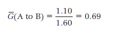
Reflection Density
In the evaluation of photographic papers, it is necessary to measure reflection densities. Reflection density is defined as the logarithm of the reciprocal of reflectance (R), where:
 (Eq. 5-10)
Thus, reflection density is defined as
The design of a densitometer that measures reflection density necessarily differs from that of a transmission instrument. Since prints are usually illuminated at an angle of approximately 45° and viewed on a plane nearly perpendicular to the image, ANSI has standardized this illumination and collection geometry, and all reflection densitometers are based upon it. If the instrument is zeroed on an unexposed, developed, and fixed-out piece of photographic paper, the base plus fog automatically will be subtracted from all future readings. When the instrument is calibrated on a reference white such as magnesium oxide, the readings will include the base-plus-fog density. Both approaches are commonly used.
Paper Characteristic Curves
Figure 5-20 contains a characteristic curve typical of a photographic paper emulsion. The major differences between this curve and that of a pictorial film are as follows:
1.The toe portion is usually longer and extends to a higher density.
2.The slope in the midsection is much steeper, and the straight-line portion is short if present at all.
3.The shoulder quickly reaches a maximum density, which is seldom more than 2.1.
Because of these conditions, the useful log exposure range of photographic paper is substantially less
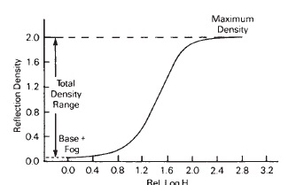
Figure 5-20 Typical characteristic curve for a black-and-white photographic paper.
than that of pictorial film. However, the purpose of photographic paper is to receive the transmitted tones of the negative as input, while the purpose of negative film is to receive the reflected tones of the original scene as input. When evaluating the contrast of photographic papers, two types of information are important—the total density (output) range and the useful log exposure (input) range.
Paper Contrast
The total density range of a paper is the range from paper base plus fog to the maximum obtainable density (sometimes called maximum black) at the top of the shoulder, as illustrated in Figure 5-20. The minimum density (base plus fog) is determined by the whiteness of the support and the fog picked up during processing. Reflection densities of 0.01 to 0.03 are typical minimum densities. The maximum obtainable density is in part governed by the emulsion type but primarily controlled by the print’s surface characteristics. A paper with a high-gloss surface can give a maximum density of about 2.10, whereas some papers identified as “glossy" may produce a density no higher than 1.90. Resin-coated papers seldom exceed 2.0. Matte surface papers show a maximum density of about 1.60.
A total density range could also be determined for an inkjet or laser photo-grade paper, although these values are not commonly provided in the manufacturer’s literature. The minimum densities are similar to emulsion-based papers. The maximum density achievable with current inks can get as high as a density of 3.0 with a high-gloss surface.
The limit on print density is associated with first-surface reflections,

Figure 5-21 First-surface reflection properties of glossy and matte surface papers.
as shown in Figure 5-21. In a typical print-viewing situation, the print is illuminated at 45° and viewed on the perpendicular. For the maximum black patch with the glossy surface, the first-surface reflection is very directional, with the angle of reflectance nearly equal to the angle of incidence. With the eye positioned as shown, the fraction of the light being reflected will not be detected. Since the incident light is either absorbed by the image or reflected at an angle where it is not readily seen, the patch appears black and consequently has a high density. When considering the maximum black patch with a matte surface, it can be seen that the first-surface reflection is quite diffuse and some light will be reflected back to the eye regardless of the viewing angle. The result is a lightening of the maximum black and a corresponding loss in maximum density. The effect on curve shape of different surfaces for the same grade of paper is shown in Figure 5-22, which demonstrates that the greatest change occurs in the shoulder. The practical consequence of this condition is that the output range of a photographic paper is controlled primarily by the surface characteristics.
Increasing the developing time of black-and-white papers beyond the minimum recommended time has little effect on the slope of the characteristic curve.
Figure 5-22 The effect of surface characteristics on the curve shape for the same grade of paper.
Unlike the negative film emulsions studied previously, the contrast of photographic papers is not readily controlled by development. Because development occurs rapidly as a result of using a high activity developer, the basic curve shape is essentially determined after a brief period. The curves in Figure 5-23 result from varying development time, with 1Vi minutes considered normal. Although it is apparent that the slope of the curves is changing, development times less than 1 minute tend to give a lowered maximum density with a mottled appearance and, therefore, unusable images. At a development time of 1 minute the curve shape is nearly fixed, with increases in development time merely shifting the curve to the left. Thus extended development times don’t change the contrast of photographic papers but do increase the speed up to about one stop. If the development time becomes too long, the fog density increases and makes the highlights appear unacceptably gray.
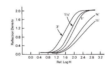
Figure 5-23 The effect of different development times on curve shape for the same grade paper.
The effects of changing development time on photographic papers may be summarized as follows:
1.Underdevelopment is to be avoided because of the lack of maximum black and the possibility of mottling.
2.Overdevelopment can be used to increase the speed by as much as one stop, but care must be taken to avoid an unacceptable increase in fog density, which ruins the white areas of the print.
3.Since the curve shape is determined early in development, changes in development conditions cannot compensate for an incorrectly chosen grade of paper.
Thus far in our analysis of photographic paper curves we have only considered the output (density) characteristics. To evaluate the input properties

Figure 5-24 The location of minimum and maximum useful points, and the resulting useful log exposure range.
requires a determination of the paper’s useful log exposure range. As with camera films the minimum and maximum useful points must be located on the curve. The location of these points is based upon the visual quality of the highlights and shadows produced in the print. Because the tones in the negative are reversed in the print, the highlights are reproduced in the toe area and the shadows in the shoulder of the paper’s characteristic curve. Therefore, the minimum useful point in the toe will be based upon proper highlight reproduction. Experiments show that non-specular highlights in a subject, such as reflections from white surfaces, should be reproduced with a density slightly greater than the base white of the paper. A density of 0.04 above base plus fog is sufficient to give a just-noticeable tonal difference above the base white of the paper, and it identifies the minimum useful point in the toe as shown in Figure 5-24. The base white of the paper is the tone that is reserved for reproducing light sources or the specular (glare) reflections from polished metal or other shiny surfaces. Since these are the brightest parts of the subject, it makes sense that they should be printed at the lightest tone possible.
When considering the reproduction of shadows and thus the maximum useful point, it is necessary to determine the desired amount of shadow detail. Again, many experiments indicate that black-and-white prints judged as excellent consistently exhibit good shadow detail. Those same experiments show that the maximum density of the print was not used to reproduce the shadow detail. Rather, a point farther down on the shoulder is used where there is sufficient slope for maintaining tonal separation. This point is typically located at a density equal to 90% of the maximum density and denotes the maximum useful point on the curve. However, portions of a scene that are very dark and contain no detail of interest are printed at the maximum density so that they may be reproduced as a solid black in the print. To summarize:
1.The minimum useful point in the toe is based on the reproduction of non-specular highlights and is located at a density of 0.04 above the paper’s base plus fog.
2.The maximum useful point in the shoulder is based on the reproduction of shadow detail and is located at a density equal to 90% of the maximum density.
3.The log exposure interval between the two points is defined as the useful log exposure range (sometimes just log exposure range) of the paper. For example, in Figure 5-24 the log exposure range was determined to be 1.10.
Although there are no exposures associated with inkjet or laser papers, the knowledge of shadow and highlight reproduction still applies. Non-specular highlights should be reproduced at 0.4 above paper white. Shadow detail is best placed at 90% of the maximum density the ink or toner can reproduce.
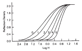
Figure 5-25 Characteristic curves for a family of papers of different contrast grades with the same surface.
Family of Paper Curves
The characteristic curves for a family of papers of different contrast grades are illustrated in Figure 5-25. The major difference between the curves is in the range of log exposures over which they extend. A grade 0 emulsion (sometimes referred to as a “soft” paper) responds over a long range of log exposures, while a grade 5 (sometimes referred to as a “hard” paper) covers a much shorter log range. All of the grades are capable of generating the same output range of densities because they all have the same minimum and maximum densities, assuming the paper surfaces are the same. The contrast grade numbers 0, 1, 2, 3, 4, and 5 represent a system for classifying the contrast of a paper based upon the log exposure range. Some manufacturers use the ANSI standard terms for describing emulsion contrasts. Table 5-4 contains the contrast grade numbers and ANSI standard terms that relate to the log exposure range. Notice that each grade of paper can have a variety of log exposure ranges. For example, a grade 2 paper
Table 5-4 Relationship between paper grade, paper log exposure range, and density range of negatives for diffusion and condenser enlargers
| Contrast Grade Number of Paper | ANSI Descriptive Term |
Log Exposure Range of Paper | Density Range of Negative Usually Suitable for Each Log Exposure Range or Grade Number (Diffusion Enlarger) | Density Range of Negative Usually Suitable for Each Log Exposure Range or Grade Number (Condenser Enlarger) |
| 0 | Very Soft | 1.40 to 1.70 | 1.41 and higher | 1.06 and higher |
| 1 | Soft | 1.15 to 1.40 | 1.15 to 1.40 | 0.86 to 1.05 |
| 2 | Medium | 0.95 to 1.14 | 0.95 to 1.14 | 0.71 to 0.85 |
| 3 | Hard | 0.80 to 0.94 | 0.80 to 0.94 | 0.60 to 0.70 |
| 4 | Very Hard | 0.65 to 0.79 | 0.65 to 0.79 | 0.49 to 0.59 |
| 5 | Extra Hard | 0.50 to 0.64 | 0.64 and lower | 0.48 and lower |
can have a log exposure range of 0.95 to 1.15, which no doubt explains at least some of the differences between papers of the same grade and surface from different manufacturers.
The American National Standard governing the sensitometric properties of black-and-white reflection print materials specifies the use of the Standard Paper Range Number (R) in lieu of the useful log exposure range. The value of R is determined by multiplying the useful log exposure range (rounded to the nearest 0.10) by 100. For example, if the useful log exposure range for a certain grade of paper is 1.07, it would be rounded to 1.10 and multiplied by 100, giving R = 110. The resulting R-value has no standard relationship to the grade numbers assigned by the manufacturers to their products and, therefore, does not reduce the differences between the same grade of paper from different manufacturers.
It should be evident by now that the density range of the negative relates to the log exposure range of the paper it is to be printed on. In fact, the negative’s density range actually determines the range of log exposures the paper will receive, and thus the paper grade required. For example,
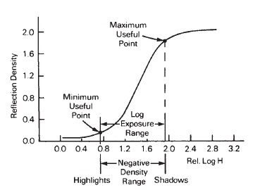
Figure 5-26 The relationship between the density range of the negative and the useful log exposure range of the paper for a correctly exposed print.
a contrasty negative is characterized by a large density range, and so it requires a soft grade of paper that can respond over an equally large range of log exposures.
Prints made on different brands of contrast grade 2 printing papers will not necessarily have the same print contrast.
This situation is illustrated in Figure 5-26, where the density range of the negative is the same as the log exposure range of the paper, and the print has been correctly exposed. The non-specular highlight in the negative will produce a density of approximately 0.04 above the base white of the paper, and the detailed shadow area of the negative will generate a density near 90% of the maximum black.
The best print quality will generally occur when the density range of the negative equals the log exposure range of the paper.
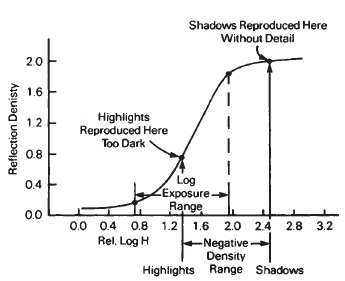
Figure 5-27 Correct match of negative density range and paper log exposure range, with print overexposed by two stops.

Figure 5-28 Negative printed on a paper grade that is too hard, printed for the shadows.
If the same negative and paper grade were used again, with a two-stop increase in print exposure, the condition illustrated in Figure 5-27 occurs. The result is a print without tonal separation in the shadows, as the shadow densities in the negative are located too far into the shoulder of the paper. Also, the highlights will be too dark because the highlight densities in the negative will print too high on the toe of the paper curve. If the same negative is printed on a grade of paper that is too hard, the condition in Figure 5-28 results. Here the print exposure has been adjusted to give adequate shadow detail, as the shadow densities of the negative are printing at the maximum useful point. However, the highlight densities extend far to the left of the minimum useful point with a complete blocking up of the print highlights. If the print exposure is increased to give better highlight reproduction, the shadows will print too far into the shoulder and begin to block up. Consequently, the odds of achieving a good print with this combination are slim. At this point, we can summarize by saying that for pictorial images, the best print quality will generally occur when the density range of the negative equals the log exposure range of the paper, and the print is correctly exposed.
Condenser and Diffusion Enlargers
The two basic types of enlargers are diffusion and condenser. The diffusion enlarger employs a large integrating sphere or ground glass to illuminate the negative with scattered light, and is classified as a diffuse system. The condenser enlarger uses a set of lenses (condensers) above the negative so that the light from the bulb will be more concentrated when it strikes the negative, and is thus a specular system. When determining a negative’s density range for the purpose of selecting the proper grade of paper, the similarity between the optical designs of the densitometer and the enlarger should be considered.
Since nearly all commercially available densitometers measure diffuse density, the resulting values usually can be directly applied to diffusion enlargers. However, as discussed earlier in this chapter, black-and-white negatives have greater density and contrast in a specular system. Consequently, the densities obtained from a diffuse-reading densitometer must be adjusted upward to convert them to specular densities. The exact value of this conversion factor (also referred to as a Q-factor) will depend primarily on the specularity of the enlarger and is best determined by testing the specific equipment. Many tests of condenser enlargers indicate that this factor is approximately 1.3. This means, for example, that a negative with a diffuse density range of 1.10 will actually have a density range of 1.43 (1.10 X 1.3) in a condenser enlarger. To compensate for this discrepancy, Table 5-4 lists the diffuse density ranges for negatives when printing in either diffusion or condenser enlargers. Notice that the diffuse density range of a negative to be printed on a grade 2 paper in a diffusion enlarger can be between 0.95 and 1.14, while the diffuse density range of a negative to be printed on a grade 2 paper in a condenser enlarger is between 0.71 and 0.85.
The curves in Figure 5-29 show the difference in print contrast between a diffusion enlarger and a condenser enlarger equipped first with an opal bulb and then with a clear bulb, using a negative made on a coarse-grained film.
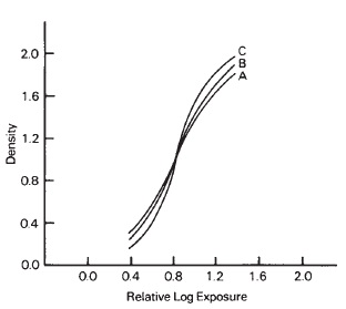
Figure 5-29 Tone reproduction curves for three prints made from the same coarsegrained negative on the same enlarging paper. (A) Diffusion enlarger. (B) Condenser enlarger with opal bulb. (C) Condenser enlarger with clear bulb.
The Effects of Enlarger Flare and Scattered Light
Flare light reduces contrast in the enlarger as well as in the camera. With cameras, shadow contrast and detail are reduced by flare, but with enlargers the highlights are most affected (except with reversal processes).
Flare light in an enlarger originates with the light that bounces around inside the enlarger body and lens before reaching the printing paper as a uniform level of light. The amount of enlarger flare light will vary with the efficiency of the lens coating and the enlarger light-baffling system, and with the proportion of shadow-to-high-light areas in the negative. It will also depend upon whether the opening in the negative carrier is masked down to the area of the negative that is actually being printed. Because enlarger flare reduces the contrast primarily in the highlight areas, it is more damaging to the image quality when it is excessive than camera flare, which reduces contrast mostly in the shadow areas.
To minimize a loss of contrast due to flare light when using an enlarger, the negative should be masked down to the area being printed.
Testing Enlargers for Flare Light
The existence of flare light in an enlarger and its effect on the output density range of the resulting print can be demonstrated easily. A projection print from a step tablet can be made with and without masking off the area around the step tablet. A side-by-side comparison of the prints will reveal differences between the two images. Measuring the density of each step with a reflection densitometer enables the construction of characteristic curves demonstrating the differences graphically, as shown in Figure 5-30.
Enlarger flare light, or intentional flashing, can improve the quality of prints made from contrasty negatives.
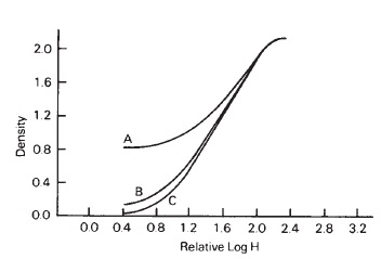
Figure 5-30 Characteristic curves showing the effects of masking off the area around a step tablet in an enlarger negative carrier. (A) No masking. (B) Masked down to a quarter-inch of the step tablet. (C) Masked down to the edge of the step tablet.
Curve A represents a high flare situation in which the area around the step tablet was not masked off. The excess area was masked down to within a quarter of an inch of the step tablet for curve B, and completely masked for curve C. It is evident that the enlarger flare most affects the print’s lighter tones, and that the flare density increases dramatically with the size of the unmasked area around the step tablet.
In some prints, the decreased image contrast produced by enlarger flare light results in improved image quality. In these prints, the contrast would have been too high without the flare light. Thus the availability of controlled, variable flare light can be useful.
Paper Speeds
The speed of a photographic paper is inversely related to the minimum exposure necessary to achieve an excellent print. As was shown to be the case in the earlier discussion of pictorial film speeds, experimental evidence indicates that print exposure should be based upon shadow detail reproduction. Since the shadows fall on the shoulder of the paper curve, the maximum useful point, located at 90%
Table 5-5 Speeds for a family of paper grades
| Contrast Grade Number of Paper | Shadow Speed | ANSI Paper Speed |
| 0 | 5000 | 1600 |
| 1 | 4000 | 1000 |
| 2 | 2500 | 500 |
| 3 | 2000 | 300 |
| 4 | 1600 | 200 |
| 5 | 1280 | 160 |
of the maximum density, is used as the speed point. The speed is referred to as a shadow speed, with the following formula being used:
where H = the exposure in lux-sec-onds needed to generate a density that is 90% of D max, and 10,000 = a large constant that will convert the speed values to a convenient size.
The shadow speeds of the curves for the family of paper grades illustrated in Figure 5-25 are shown in Table 5-5, which indicates that the shadow speed decreases as the contrast of the paper (paper grade) increases. This means that a grade-4 paper is slower than a grade-2, and appropriate compensation must be made in the exposure time when changing paper grades. The actual speeds of various brands of the same grades of paper will be different, but the general relationship is that the higher the paper grade, the slower the speed.
An alternative method for determining the paper speed is based upon the exposure necessary to produce a mid-tone with a density of 0.60 above base plus fog. This is the current ANSI-standard procedure for deriving the paper speed and is predicated on the assumption that proper mid-tone reproduction is most important. The resulting speed value is called the ANSI Paper Speed (sometimes ASAP) and is based on the following formula:
 (Eq. 5-13)
where H = the exposure in lux-seconds needed to generate a density of 0.60 above base plus fog, and 1,000 = a large constant that will convert the speed value to a convenient size.
Table 5-5 shows a comparison of Shadow Speeds and ANSI Paper Speeds for six grades of paper. If print exposure times are based on the speed numbers when changing paper grades, Shadow Speeds will produce matched shadow densities and ANSI Paper Speeds will produce matched mid-tone densities. Some brands of photographic paper show curves similar to those illustrated in Figure 5-31. Since all the curves cross at a density of 0.60 above base plus fog, they will all show the same ANSI Paper Speed. The shadow speed obviously will be different since the position of the shoulder is changing. When printing to a mid-tone with these emulsions,
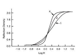
Figure 5-31 Family of paper contrast grades showing the same ANSI paper speed but different shadow speeds.
no change in print exposure would be required as a function of changing paper grades. However, when printing for the shadows, significant changes in print exposure would be needed when changing grades. Paper speed numbers can be used to calculate the new printing exposure time when changing from one paper to another. Conversion tables or dials are also available from some paper manufacturers.
Traditionally, low-contrast grades of printing paper have had higher speeds than high-contrast grades.
Analysis of Positive Film Curves
An alternative to printing on photographic paper is to use a relatively high-contrast film, which will yield a positive transparent image that can be viewed by either back illumination or projection. The films used for this purpose are called film positive emulsions or release print films. They typically have slow speed, very fine grain, and inherently high contrast with gammas varying between 1.8 and 2.8, depending upon the developer formulation and development time. The characteristic curve for such an emulsion is shown in Figure 5-32, where it can be seen that the slope is quite steep.
In principle, the production of film positives from negatives is similar to

Figure 5-32 The characteristic curve of a film positive emulsion.
that of reflection prints except that the contrast of the emulsion being printed upon can be controlled readily by development. This eliminates the need for various contrast grades. Experience indicates that the minimum useful point on the film positive curve for good highlight reproduction is approximately 0.30 above the density of base plus fog. If the highlights are reproduced with a greater density than this, they appear too dark, and if the density is any less, they look “washed out.” Although these films are capable of achieving densities over 3.0, the shadows are best reproduced at densities of 2.7 and less depending upon the contrast of the negative. The larger density range available with film positives is far greater than that of photographic paper allowing subjects with high luminance ratios to be faithfully reproduced. The relationship between the density range of the negative and the film positive curve is illustrated in Figure 5-33 for a correctly exposed and processed image.
Negatives can be printed onto print film materials to obtain positive images on a transparent base that can be viewed by projection or with transmitted light from an illuminator.

Figure 5-33 The relationship between the density range of the negative and the useful log exposure range of the film positive emulsion for a correctly exposed image.
Notice that the slopes in both the highlight and shadow regions of the curve are greater than those of a photographic paper. The resulting film positive will have greater tonal separation in those areas than a reflection print made from the same negative.
There is no standard method for determining the speed of positive films, but speed points based upon either highlight or shadow reproduction are commonly used to calculate speed values. The highlight method involves determining the exposure necessary to produce 0.3 above base-plus-fog density using the following formula:
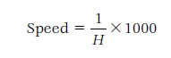 (Eq. 5-14)
The mid-tone method employs the same formula, except that the exposure necessary to generate a density of 1.0 above base plus fog is used. Shadow speeds are seldom used for these films because the steep slope in the shadow region of the curve assures that good shadow detail will be maintained. Therefore, print exposures are generally based upon either highlight detail or mid-tone density. Regardless of which speed method is used, the speed of film positive emulsions is highly dependent upon the degree of development. Figure 5-34 shows a family of curves for different development times of a film positive emulsion. The curve shifts to the left, indicating an increase in speed, as development time lengthens. Thus close attention must be given to the details of development if consistent results are to be obtained.
By printing on film positive emulsions, the photographer can overcome the single greatest limitation of the negative-positive system—the low maximum density produced by photographic papers. The wider density
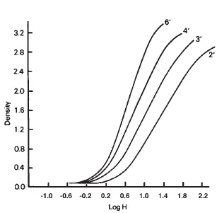
Figure 5-34 Characteristic curves for a variety of development times of a film positive emulsion.
range of the film positive results in images with greater physical and visual contrast. Not only will the tonal range appear greater, but also the shadows and highlights will have more detail and brilliance. Ideally, film positives should be viewed on a transparency lluminator in a darkened room with he surround masked off to obtain the greatest visual contrast. If the image s placed in a projector and viewed on a screen under typical conditions, the mage contrast is drastically reduced as a result of both optical flare and ambient room light reaching the screen. Even under these conditions, the con-rast of projected images still exceeds that of reflection print images.
Analysis of Reversal Film Curves
The generation of a positive, transparent image may also be accomplished hrough a procedure called reversal processing. In this method, a film hat was exposed in the camera is first developed to a negative, without fixing. In the next step, a bleach bath dissolves the negative silver image

Figure 5-35 Characteristic curve of a reversally processed film.
leaving unexposed silver halide in amounts opposite to those of the negative. This unexposed silver halide is exposed (fogged) by flashing to light (or is chemically fogged) and then developed to give the desired positive image. The second development is followed by fixation, washing, and drying. The result is a black-and-white transparency produced on the original film exposed in the camera.
The basic steps of reversal processing are to develop a negative image, bleach the negative image, fog the remaining silver halides, and develop the positive image.
The characteristic curves for reversal materials are plotted in the same manner as those of negative working emulsions except that the direction of the curve is reversed. This is necessary because with reversal materials the density decreases as the exposure becomes larger. Consequently, the shadows and darker tones are reproduced as high densities while the highlights and lighter tones yield small densities. The D-log H curve for a typical reversally processed film is shown in Figure 5-35. The curve exhibits a steep middle section, which is necessary to give sufficient contrast to the image, since it will be viewed directly. This results in a shortened useful log exposure range, meaning that the exposure latitude is small and scenes with excessive contrast cannot be properly reproduced. In fact, most reversally
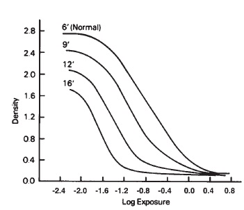
Figure 5-36 The characteristic curves resulting from different first development times for reversally processed film.
processed emulsions do not exceed a 1.90 useful log exposure range. Although many negative-working films may be reversally processed, emulsion manufacturers usually design or designate specific films to be processed using the reversal method.
The influence of processing changes on the curve shape is more difficult to ascertain with reversal processing because there are more major steps involved than with negative processing. The effect of varying the time of first development while all other steps are held constant is illustrated in Figure 5-36. The first development time has a significant effect upon all of the sensitometric parameters of the film. As the first development time is lengthened, the maximum density of the positive image becomes lower due to an increase in the fog density at the negative stage. The minimum density also decreases slightly because of the increase in the shoulder density at the negative stage. Increases in the slope of the curve are most noticeable in the toe region, indicating a small gain in contrast.
The effect on speed of altering the first development time is shown

Figure 5-37 First development time vs. film speed for reversally processed film.
in Figure 5-37. The speed point was located at a density of 1.0 above base plus fog, and the speed was calculated using the following formula:
The graph indicates that the speed of reversally processed films can be increased by up to 10 times by lengthening the time in the first developer. However, the speed increase is coupled with a decrease in the maximum obtainable density, which results in poor shadow reproduction. When the maximum density falls below 2.0 for transparencies, shadow-detail reproduction is usually unacceptable. The increased contrast in the midtones may also contribute to an inferior result.
Introduction to Photographic Effects
Most of the time, the response characteristics of photographic materials and processes are quite predictable, based on the principles discussed thus far. However, there are conditions where the resulting photographic image does not have the characteristics that were anticipated. Although the making of photographs is a relatively simple task, the response properties of photographic materials are quite complicated. An understanding of conditions that can lead to unexpected results will be most beneficial in mastering the photographic process. Some of these photographic effects are considered in the sections that follow.
Reciprocity Effects
Photographic effects can produce unexpected responses to exposure of photographic materials.
In 1862, two scientists, Robert Wilhelm Bunsen and Henry Enfield Roscoe, proposed a general law for photochemical reactions stating that the end result of a primary photochemical reaction simply depends upon the total energy used, regardless of the rate at which the energy is supplied. Photography involves a photochemical reaction in which light is used to expose film or paper to form a usable latent image, and chemistry is used to develop a visible silver or dye image. The end product (density), however, does not depend simply upon the total energy (exposure), but also on how that exposure is distributed in terms of illuminance and time. For example, two pieces of film can receive equal exposures that may result in different densities because the exposure times and illuminances are quite different. Exposure (H) is a product of illuminance (E) and time (t). An illuminance of 2 lux for 1/100 second produces the same exposure (0.02 lux seconds) as an illuminance of 0.002 lux for 10 seconds. Because the response may be different for these two exposures, the reciprocity law of Bunsen and Roscoe is said to have failed.
Early literature described this situation as reciprocity law failure (RLF). Current literature simply refers to it as reciprocity failure or reciprocity effect to distinguish it from Bunsen and Roscoe’s reciprocity law, which holds true for primary photochemical reactions. The law is considered valid for X-ray and gamma ray exposures with silver halide emulsions, and for light exposures with certain non-silver processes such as diazo and selenium electrostatic processes. Reciprocity failure in photography simply means that the response (density) of a photographic material cannot be predicted solely from the total exposure a film has received (except over a small range of exposure times). For pictorial films, the range over which reciprocity failure is negligible is from about 1/10 second to about 1/1,000 second. Beyond these time limits reciprocal combinations of exposure time and illuminance that give the same total exposure will not give the same density response. As an example, if a meter indicates camera exposure settings of f/5.6 and 1/30 second, but because greater depth of field is needed the lens is stopped down to f/45 and the film is exposed for 2 seconds, the resulting densities will not be the same even though the combinations of camera settings were equivalent. The 2 second exposure will result in a thinner negative. Density will be less for exposure times longer than 1/10 second or shorter than 1/1,000 second. In other words, the film will be underexposed even though the subject was metered correctly, the right camera settings were used, and development was correct. This is an example of reciprocity failure or the reciprocity effect.
Low-illuminance reciprocity failure typically results in a decrease in negative density and an increase in contrast.
In addition to the loss in density already noted, reciprocity failure can change image contrast. The extent of
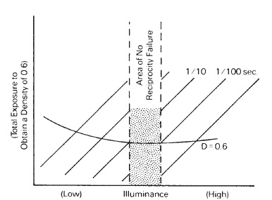
Figure 5-38 Reciprocity curve. A straight horizontal line would represent no reciprocity failure.
the changes in density and contrast depends upon the combination of illuminance and exposure time and the characteristics of the emulsion. The reciprocity curve in Figure 5-38 shows the relationship between the total exposure (on the vertical axis) required to obtain a given density of 0.6 and the various combinations of illuminance (horizontal axis) and time (45 lines). If there were no reciprocity failure, the curve would be a straight horizontal line, and the same exposure, regardless of the reciprocal combinations of illuminance and time used, would give the same density. This is true over a limited range of illuminances and times as indicated by the bottom part of the curve, which is almost flat. (Although reciprocity curves will generally differ from one product to the next, they will have the same shape except for certain special emulsions.)
Low-Illuminance Film Reciprocity
Reciprocity failure is often encountered in low-light-level photography, and it is commonly the reason for thin, underexposed negatives. The sensitometric effect of low-illuminance reciprocity failure for a pictorial film can be seen

Figure 5-39 Low-illuminance (long exposure time) reciprocity failure.
in Figure 5-39. All three films were given the same exposure, employing reciprocal values of illuminance and time to allow the use of three different exposure times. The same conditions of development were used for each. If there were no reciprocity failure, the three curves would have the same shape and be superimposed. The fact that the 1-second and 10-second curves are displaced rightward indicates a progressive loss of film speed as the exposure time increases. In other words, when using exposure times of 1 second and longer for this emulsion, additional exposure is required to obtain the expected image density.
Adjustments need to be made in development as well as exposure for long exposure times at low light levels. The reason for this can be seen in Figure 5-39. In addition to the displacement of the curves, the curves differ in slope.
As the exposure times reach 1 second and longer, there is a significant increase in slope and thus image contrast. Whereas an exposure time of 1/100 second with normal development produced a contrast index of 0.63, an exposure time of 10 seconds with the same normal development produced a negative with a contrast index of 0.82—about a 30% increase in contrast. This is caused by the fact that low-intensity reciprocity failure affects the lower density areas more than the higher density areas. Thus, in order to obtain the expected image contrast in the negative, a reduction in development is necessary. Because altering the degree of development also affects density, the reciprocity failure exposure factor will be larger than it would be if the degree of development is not adjusted for the anticipated increase in contrast with long exposure times.
Low-illuminance reciprocity failure requires an increase in exposure along with a decrease in development to adjust for contrast. If only the exposure correction is made, the negative may have to be printed on a lower grade of paper than usual to adjust for the increase in contrast index of the negative.
High-Illuminance Film Reciprocity
Exposure of films for times shorter than 1/1,000 second, as with some electronic flash units, results in decreased density. The decrease is largest in the highlight areas, with negative type films producing a lower-contrast image. An exposure increase and an increase in development are both needed to compensate for this.
The characteristic curves in Figure 5-40 illustrate the effect of high-illuminance reciprocity failure. All three films received the same total exposures, using reciprocal values of illuminance and time to obtain shorter exposure times. Development conditions were kept constant. Notice that the 1/10,000- and 1/100,000-second curves are also displaced rightward, indicating a loss of film speed. It is important to notice that under these

Figure 5-40 High-illuminance (short exposure time) reciprocity failure.
conditions the curve shape changes in a manner opposite to that with low illuminance. Specifically, the slope of the curve decreases at exposure times of 1/10,000 second and less, indicating a loss of contrast. Observe, however, that contrast increases with increasing exposure time, for both low-illuminance and high-illuminance reciprocity failure. If only an exposure adjustment is made, the negative would have to be printed on a higher contrast
High-illuminance reciprocity failure typically results in a decrease in negative density and contrast.
Black-and-White Paper Reciprocity
Reciprocity effects are exhibited by all photographic emulsions and can be seen easily by printing on any photographic paper and using a series of increasing exposure times, as shown in Figure 5-41. A photographic step tablet was first printed at a relatively short exposure time of 10 seconds at f/5.6, and then for each subsequent print the exposure time was increased as the illuminance was proportionally decreased by stopping the lens down and adding neutral density filters. The density decreased progressively even though each test strip received the same series of photographic exposures—as the illuminance
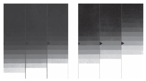
Figure 5-41 The three prints of a film step tablet on two different types of photographic paper all received the same photographic exposure but with decreasing illuminances and increasing exposure times from left to right. The decreasing densities with increasing exposure times are the result of reciprocity effects, with the paper on the right showing a more dramatic change.
decreased, the exposure time increased, and the development remained the same.
Noticeable reciprocity failure with printing papers is seldom encountered when using normal negatives. It is a problem, however, when printing a severely overexposed and/or overdeveloped negative to a large magnification. With the aperture wide open, the usual way to increase exposure is by lengthening print exposure time. Because of reciprocity failure, increasing print exposure times does not give the expected increase in image density.
Reciprocity failure with some color materials can cause a change in color balance, as well as a loss in density.
Reciprocity failure also presents a problem when a high-density area in the negative has to be manipulated by burning-in or where high magnifications are required such as in printing photomurals or in printing small areas of a negative to a large print size.
In addition to a loss in speed with printing-paper reciprocity failure, one can also expect a loss in contrast. This is illustrated in Figure 5-4. The 240-second (4-minute) curve has been adjusted for the speed loss so that the loss in contrast is more apparent.

Figure 5-42 Excessively long printing times result in a decrease in paper contrast as well as speed. (The loss in paper speed has been adjusted to emphasize the loss in contrast.)
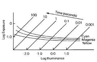
Figure 5-43 Reciprocity failure for a reversal color film. The reciprocity characteristics are made to match over a limited range of exposure times. Beyond those times the three different emulsions exhibit different degrees of reciprocity failure.
Whereas one can expect reciprocity failure to cause an increase in contrast for films exposed for relatively long times (low illuminances), a decrease in contrast for print papers can be expected.
Color Film Reciprocity
Figure 5-43 illustrates reciprocity failure curves for a color reversal film. The curves represent constant density lines for the cyan, magenta, and yellow dye layers of the film. Multilayer color films require the balancing of at least three different emulsions so that their reciprocity failure characteristics, over an extended range of exposure times, are similar. For the color film represented in Figure 5-43, the reciprocity failure characteristics are similar over a range of exposure times between approximately 1/10 and 1/1,000 second. (This assumes that processing is in accordance with the manufacturer’s recommendations.) When exposure times longer than 1/10 second are used, adjustments to the exposure given each of the three layers must be made. This is usually done by adding the proper color filter and increasing the exposure.
Film manufacturers have had considerable success in modifying reciprocity effects with alterations of the film and paper emulsions in recent years so that most contemporary films and papers suffer much smaller changes in image density, contrast, and color balance than films and papers produced previously.
Sabattier Effect
Photographic film or paper that is partially exposed to image-forming light and partially developed (but not fixed) can, if reexposed with uniform illumination, developed, and fixed, result in a partial reversal of tones. The reversal is most noticeable in the areas receiving the least exposure: the shadow areas for film and the highlight areas for paper. In addition to a partial reversal, the edge or contour of a shape is often strongly enhanced. This dark line effect, referred to as a Mackie line, and partial reversal of tones can be seen in Figure 5-44. To obtain the Sabattier effect, no special equipment or solutions of any kind are required:
1.Give the film or paper a somewhat less than normal image exposure.
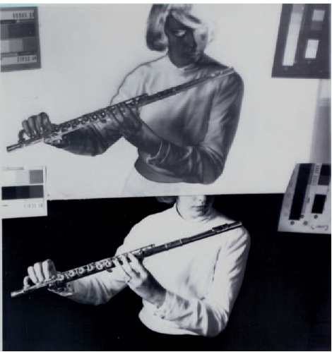
Figure 5-44 The Sabattier effect (top). Note the partial reversal of tones and the black line along some of the contour.
2.Develop for about half the normal development time.
3.Rinse in water (do not use a stop-bath or fixing solution).
4.Reexpose by fogging to light for a brief time.
5.Return the film or paper to the developer and develop for the other half of the normal time.
6.Rinse, fix, wash, and dry as you normally would.
Man Ray accidentally rediscovered the Sabattier effect and incorrectly labeled it solarization.
Note that for single sheets of film or paper, the rinse step can be eliminated. The second exposure can be made while the film or paper is in the developer. Allow the solution to settle for about 10 seconds, however, before making the second exposure.
Some experimentation may be required to get the desired results. The
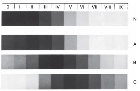
Figure 5-45 Gray scales showing the Sabattier effect. Gray-scale prints made from Kodak Super XX Pan Film processed for various combinations of first and second development times. (Films all received the same first and second exposures.)
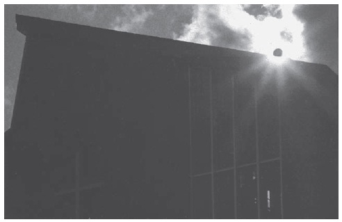
Figure 5-46 An example of solarization caused by extreme overexposure of the sun. (Photograph by Leslie Stroebel).
ratios of first to second exposures and first to second developing times are important variables. Figure 5-45 shows that decreasing the first development time and increasing the second development time while keeping the fogging reexposure constant increases the amount of tone reversal.
Some modern films are difficult to solarize, especially if processed in a developer containing a silver-halide solvent.
Development Times
| Gray Scale | 1st Dev. | 2nd Dev. | Total (minutes) |
| N | 6 | 0 | 6 |
| A | 4 | 2 | 6 |
| B | 3 | 3 | 6 |
| C | 2 | 4 | 6 |
The Sabattier effect can appear if the fogging exposure is accidentally given during first development, as with unsafe “safelights." Applications of this effect have mainly been associated with interesting pictorial effects, but the line effect has been used, for example, to enhance the sharpness of spectrographic images. When the Sabattier effect is used with color negative or reversal materials, changes in hues, lightness, and saturation can be produced by varying the spectral energy distributions of the two exposures.2
Solarization
Increasing exposure increases density until a maximum density is reached. Extreme overexposure can result in a loss of density and reversal of the heavily exposed areas. Figure 5-46 shows a severely overexposed negative that resulted in a complete reversal of the sun. The degree of solarization depends on the particular film or paper and the developer used.
2 Eastman Kodak Co., Darkroom Expressions, 1984, p. 64.
REVIEW QUESTIONS
1.In tone reproduction studies, the term input data refers to information about the …
- subject
- image
- type of meter
- exposure
- film development
2.A subject has a highlight luminance of 200 c/sq.ft and a shadow luminance of 0.50 c/sq.ft. The luminance ratio of the scene is …
- 20:1
- 90:1
- 150:1
- 200:1
- 400:1
3.A subject luminance ratio of 200:1 corresponds to a log luminance range of …
- 1.3
- 1.7
- 1.9
- 2.3
- 3.0
4.Assume that a gray scale has been photographed, and the print made from the negative matches the original gray scale exactly. The tone reproduction curve for this situation would be …
- a straight line
- a C-shaped curve
- an S-shaped curve
5.Using current international symbols, photographic exposure is defined as …
- E = I + T
- E = I XT
- H = I XT
- H = E + T
- H = E XT
6.Photographing a gray scale with a camera is not a completely satisfactory alternative to exposing film in a sensitometer because …
- camera shutters tend to be inaccurate
- camera flare affects image illuminances
- light falls off toward the corners of the film
- all of the above
- none of the above. The camera is a satisfactory substitute for a sensitometer
7.The part of sensitometers that represents the subject is the …
- light source
- shutter
- step tablet
- filter
- adjustable diaphragm
8.The most important reason for agitating film properly during development is to …
- shorten the time of development
- produce uniform development
- keep the film wet
- increase the effective film speed
9.If 80 units of light are incident on an area of a negative and 20 units are transmitted, the transmittance is …
- 0.20
- 0.25
- 0.80
- 2.50
- 4.0
10.Density is defined as the …
- antilog of the opacity
- log of the transmittance
- log of 1/opacity
- antilog of the transmittance
- log of the opacity
11.The density that corresponds to an opacity of 8 is …
- 0.4
- 0.6
- 0.8
- 0.9
- 1.0
12.Most commercial densitometers are designed to measure …
- specular density
- diffuse density
- doubly diffuse density
13.The maximum slope of film characteristic curves occurs in the …
- toe region (only)
- shoulder region (only)
- straight line region (only)
- straight line and shoulder regions
- base-plus-fog region (only)
14.“Total negative contrast" is a synonym for …
- log exposure range
- luminance ratio
- curve slope
- density range
- Dmax plus Dmin
15.The useful log exposure range is the distance along the horizontal axis between the …
- two ends of the straight line
- two ends of the characteristic curve
- minimum and maximum useful points
16.Gamma is defined as …
- (A Log H)/(AD)
- (AD)/(A Log H)
- (AD) X (A Log H)
- (AD) + (A Log H)
17.Gamma is considered to be a measure of …
- subject contrast
- negative contrast
- printing contrast
- development contrast
- exposure contrast
18.In the relationship SPEED = 1/H, an appropriate unit for H is …
- footcandle
- second
- /-number
- lux-second
- meter-second
19.The lowest point on film curves where good shadow detail is retained is considered to be where the …
- log exposure is 0.1 above base plus fog
- slope is 0.1 above base plus fog
- density is 0.01 above base plus fog
- none of the above
20.The ISO (ASA) film speed for a film that requires .0064 lux-seconds’ exposure to produce the specified density is …
- 100
- 125
- 160
- 200
- 400
21.For proper reproduction of the darkest detailed subject shadows in reflection prints, they should be located on the paper curve at a density of …
- 0.04 above base plus fog
- 0.10 above base plus fog
- 0.60 above base plus fog
- 90% of the maximum density
- the maximum density
22.The main difference between a number 1 grade paper and a number 4 grade paper is in the …
- range of log exposures they can accept
- minimum density obtainable
- maximum density obtainable
- location of the speed point on the curve
23.For printing with diffusion enlargers, the negative density range should …
- be 0.6
- be 0.85
- match the density range of the paper
- match the log exposure range of the paper
- match the contrast index of the paper
24.Enlarger flare light affects print contrast …
- more in the highlights than in the shadows
- more in the shadows than in the highlights
- uniformly in all areas
25.The exposure time range that produces minimum reciprocity failure with pictorial films is …
- 1 sec. to 60 sec
- 1/10 sec. to 1 sec
- 1/1000 sec. to 1/10 sec
- 1/100,000 sec. to 1/1000 sec
26.To obtain the correct density and contrast with films exposed for long exposure times at low illuminance levels, it is necessary to …
- increase the exposure and increase the development
- increase the exposure and decrease the development
- decrease the exposure and increase the development
- decrease the exposure and decrease the development
- increase the exposure only
27.Mackie lines are associated with …
- the Herschel effect
- reciprocity effects
- solarization
- the Sabattier effect
- the Mackintosh effect
28.Edge effects produce …
- an increase in image sharpness
- a decrease in image sharpness
29.The by-products of development act in a manner similar to the developer ingredient identified as the …
- developing agent
- activator
- preservative
- restrainer
- solvent
30.The danger of film damage caused by static electricity is greater when the humidity is …
- high
- low
1 Ilford and Fuji use
2 Eastman Kodak Co., Darkroom Expressions,1984, p. 64.