10. Mashing Up Data with Power Pivot
In This Chapter
Understanding the Benefits and Drawbacks of Power Pivot and the Data Model
Joining Multiple Tables Using the Data Model in Regular Excel 2016
Using the Power Pivot Add-in from Excel 2016 Pro Plus
Understanding Differences Between Power Pivot and Regular Pivot Tables
Power Pivot debuted in Excel 2010 as a free add-in with six jaw-dropping features. It was an amazing product, created outside the Excel team. You’ve already seen the Data Model in Chapter 7, “Analyzing Disparate Data Sources with Pivot Tables.” The Data Model is really the Power Pivot engine, and it was first built into Excel 2013.
The Data Model gives you some of the Power Pivot features, but many more features require the Power Pivot add-in, which ships with Office 365 Pro Plus or the E3 level of Office volume licensing.
Note
If you have Office 2016 Standard, you can still use the Power Pivot engine as the Data Model, but you are locked out of the Power Pivot window and some other features. You have to upgrade to a higher version of Office 2016 to unlock these features.
Understanding the Benefits and Drawbacks of Power Pivot and the Data Model
Let’s start with the three most important benefits of Power Pivot and analyze what is in each version of Excel. These features are joining two related tables, analyzing more than 1 million records, and creating calculations using DAX.
Merging Data from Multiple Tables Without Using VLOOKUP
Everyone using Excel 2016 can merge data from multiple tables without using VLOOKUP. If you have the Standard edition, you won’t see the Power Pivot branding; rather, you’ll just be using the Data Model.
![]() To learn how to build a multitable analysis, see “Joining Multiple Tables Using the Data Model in Regular Excel 2016,” p. 226.
To learn how to build a multitable analysis, see “Joining Multiple Tables Using the Data Model in Regular Excel 2016,” p. 226.
Tip
If you have the Power Pivot add-in, building relationships is easier using a graphic view.
Importing 100 Million Rows into a Workbook
The Power Pivot grid holds unlimited rows. I’ve personally seen 100 million rows. Your only limit is the 2GB maximum file size for a workbook and available memory. Thanks to the VertiPaq compression algorithm, a 50MB text file frequently fits into 4MB when it is in the Power Pivot grid. For a 10-column data set, that means you can get about 950 million rows of data in one workbook. Loading more than 1,048,576 records is available to all versions of Excel 2016.
With Office Standard, you can import huge numbers of records and produce pivot tables; however, you aren’t allowed to browse the records. You need the Power Pivot add-in to browse. This is an intense psychological hurdle. I want to be able to see my data before reporting on it. It would be like putting a Maserati engine in a jalopy, but then welding the hood shut so I can’t actually look at the engine. Yes, I can still drive the car really fast, but I simply have this intense need to be able to browse my data. It makes me feel better. Maybe you feel the same.
Creating Better Calculations Using the DAX Formula Language
The DAX language, discussed later in this chapter, is not available in Standard editions of Excel 2016. You need the Power Pivot add-in in order to add new calculations to the Power Pivot grid and to add new calculated columns to a pivot table.
As you’ll learn shortly, the DAX language provides a lot of flexibility. Although it’s the hardest feature of Power Pivot to learn, it offers the biggest paybacks.
Other Benefits of the Power Pivot Data Model in All Editions of Excel
You get a number of other side-effect benefits of running your data through the Data Model:
![]() Count Distinct becomes a calculation option. This type of calculation was previously hard to do. Excel tricksters would add a column to the original data that divided 1 by the
Count Distinct becomes a calculation option. This type of calculation was previously hard to do. Excel tricksters would add a column to the original data that divided 1 by the COUNTIF of a field. If a customer showed up five times, the calculation would evaluate to 1/5, or 0.2. They would then add up the five records with 0.2 and to get one unique customer. If you’ve ever gone through this painful process, you will be thrilled to know that, thanks to the Data Model, Count Distinct is two clicks away. Ditto for those of you who wanted a distinct count but could never get the workaround to work.
![]() You can include filtered items in grand totals. Create a pivot table showing the top 10 customers. The grand total has always been just the 10 customers you see. Now you can make that total include all of the small customers who were filtered out of the report. This feature has always been in the Subtotals drop-down on the left side of the Design tab in the ribbon, but it was perpetually grayed out. Run your data through the Data Model, and it becomes available.
You can include filtered items in grand totals. Create a pivot table showing the top 10 customers. The grand total has always been just the 10 customers you see. Now you can make that total include all of the small customers who were filtered out of the report. This feature has always been in the Subtotals drop-down on the left side of the Design tab in the ribbon, but it was perpetually grayed out. Run your data through the Data Model, and it becomes available.
![]() Named sets were introduced in Excel 2010, but only for people with OLAP data. Named sets let you create pivot tables, for example, with last year’s actuals and next year’s budget. By taking your data through the Data Model, you cause named sets to become available.
Named sets were introduced in Excel 2010, but only for people with OLAP data. Named sets let you create pivot tables, for example, with last year’s actuals and next year’s budget. By taking your data through the Data Model, you cause named sets to become available.
![]() If you ever use the
If you ever use the GETPIVOTDATA function to extract values from pivot tables, you can save a step and convert your pivot table to cube formulas. Cut and paste these into any format desired.
Benefits of the Full Power Pivot Add-in with Excel Pro Plus
If you have Excel Pro Plus and the full Power Pivot add-in, you also have access to these features:
![]() You can access the Power Pivot grid, where you can actually browse through the 100 million rows. You can sort, filter, and add calculations in the grid.
You can access the Power Pivot grid, where you can actually browse through the 100 million rows. You can sort, filter, and add calculations in the grid.
![]() In a graphical design view, you can build relationships by dragging between fields.
In a graphical design view, you can build relationships by dragging between fields.
![]() You have the ability to change the properties of fields in the model. You can choose which fields should appear in the PivotTable Fields list and which should not.
You have the ability to change the properties of fields in the model. You can choose which fields should appear in the PivotTable Fields list and which should not.
![]() You can specify that FieldA (for example, month name) should be sorted by FieldB (for example, month number).
You can specify that FieldA (for example, month name) should be sorted by FieldB (for example, month number).
![]() You can define a default number format to use when the field appears in a pivot table. How many times have you wished for this in a regular pivot table?
You can define a default number format to use when the field appears in a pivot table. How many times have you wished for this in a regular pivot table?
![]() You can define a field as representing a product, a geographic area, or a link to an image.
You can define a field as representing a product, a geographic area, or a link to an image.
![]() You get access to a weak implementation of key performance indicators. This would be simpler to use icon sets in your resultant pivot table.
You get access to a weak implementation of key performance indicators. This would be simpler to use icon sets in your resultant pivot table.
![]() You get access to Power View dashboards. This is discussed in Chapter 11, “Dashboarding with Power View and 3D Map.”
You get access to Power View dashboards. This is discussed in Chapter 11, “Dashboarding with Power View and 3D Map.”
Understanding the Limitations of the Data Model
When you use the Data Model, you transform your regular Excel data into an OLAP model. There are annoying limitations and some benefits available to pivot tables built on OLAP models. The Excel team tried to mitigate some of the limitations for Excel 2016, but many are still present. Here are some of the limitations:
![]() Fewer calculation options—Although you now have access to Distinct Count, you lose access to other calculation options such as Product.
Fewer calculation options—Although you now have access to Distinct Count, you lose access to other calculation options such as Product.
![]() Less grouping—While Excel 2016 introduced the Auto Group feature for dates, you cannot use the Group feature of pivot tables to create territories or to group numeric values into bins.
Less grouping—While Excel 2016 introduced the Auto Group feature for dates, you cannot use the Group feature of pivot tables to create territories or to group numeric values into bins.
![]() Strange drill-down—Usually, you can double-click a cell in a pivot table and see the rows that make up that cell. This does work with the Data Model, but only for the first 1,000 rows.
Strange drill-down—Usually, you can double-click a cell in a pivot table and see the rows that make up that cell. This does work with the Data Model, but only for the first 1,000 rows.
![]() No calculated fields or calculated items—The Data Model does not support calculated fields or calculated items. If you have Power Pivot, the DAX measures run circles around those old calculations. However, if you don’t have Power Pivot, you are going to be frustrated using the Data Model.
No calculated fields or calculated items—The Data Model does not support calculated fields or calculated items. If you have Power Pivot, the DAX measures run circles around those old calculations. However, if you don’t have Power Pivot, you are going to be frustrated using the Data Model.
Joining Multiple Tables Using the Data Model in Regular Excel 2016
Microsoft faced a marketing dilemma. It had built the best features of Power Pivot right into Excel 2013, but it then tried to get customers to spend extra money for Office Pro Plus to get Power Pivot, Power View, and Inquire.
Note
Although the name Power Pivot sounds really awesome and powerful, Microsoft doesn’t include the product in the Standard edition so they had to come up with another name to describe the Power Pivot engine in Standard Excel 2016. When you see the capitalized words Data Model in Excel 2016, that is Microsoft’s way of saying you are using Power Pivot without calling it Power Pivot.
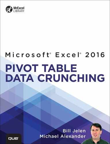
Figure 10.1 shows the Create PivotTable dialog. The Add This Data to the Data Model check box really means that you will be using the non-branded version of the Power Pivot engine.
Preparing Data for Use in the Data Model
When you are planning on using the Data Model to join multiple tables, you should always convert your Excel ranges to tables before you begin. You theoretically do not have to convert the ranges to tables, but joining the tables is far easier if you convert the ranges to tables and name the tables.
Caution
If you don’t convert the ranges to tables first, Excel secretly does it in the background and gives your tables meaningless names such as Range.
Figure 10.2 shows two ranges in Excel. Columns A:H contain a transactional data set. Columns J:K contain a customer lookup table to add an industry sector for each customer. Say that you would like to create a pivot table showing revenue by sector.

Excel gurus are thinking, “Why don’t you do a VLOOKUP to join the tables?” In this case, the tables are small and a VLOOKUP would calculate quickly. However, imagine that you have a million records in the transactional table and 10 columns in the lookup table. The VLOOKUP solution quickly becomes unwieldy. The Power Pivot engine available in the Data Model can join the tables without the overhead of VLOOKUP.
Convert the first data set to a table by following these steps:
1. Select any one cell in the first data set.
2. Press Ctrl+T or select Home, Format as Table and then select a format.
3. The Create Table dialog appears. Provided that you have no blank rows, the address will be correct. And if you have a heading above each column and three or more columns, the dialog will preselect My Table Has Headers. Make sure to check this box if it is not already checked. Click OK to convert the range to a table. You will immediately notice the AutoFilter drop-downs in each heading and that a formatting style has been applied to the first range. The formattingis not the important part. The important part is that Excel is now treating this data set like a database table. A Table Name field in the left part of the ribbon shows a table name such as Table1 (see Figure 10.3).

4. Click in the Table Name field and give the table a meaningful name. Database experts would call this the Fact table, but feel free to use Sales, Data, InvoiceRegister, or anything that describes the data. Sales is the table name for this example.
Now convert the second range to a table:
1. Select cell J1.
2. Press Ctrl+T. Ensure that My Table Has Headers is checked. Click OK.
3. Type a table name such as Sectors in the Table Name field in the ribbon.
You now have two tables defined in this workbook, and you are ready to begin building the pivot table.
Adding the First Table to the Data Model
Choose one cell in the first data set and select Insert, PivotTable from the ribbon. You can’t use the Recommended Pivot Tables or Analysis Lens options to build a Data Model pivot table.
The table name appears in the Create PivotTable dialog. Choose the check box Add This Data to the Data Model, as shown previously in Figure 10.1.
Tip
Remember that “Data Model” is the nonbranded, boring name for Power Pivot.
Click OK. Creating a Data Model pivot table takes several extra seconds as Excel converts and loads your data into the model.
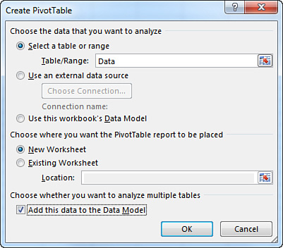
Eventually, you get a new blank workbook with a pivot table icon in A3:C20, just like with a regular pivot table. The PivotTable Fields list appears, but it is a slightly different version. In Figure 10.4, note the addition of the choice of two tabs: Active and All.
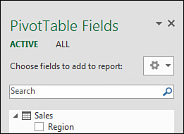
Figure 10.4 The choices for Active or All indicate that you have a pivot table that’s using the Power Pivot engine.
Expand the Sales table and choose Revenue. You see a small pivot table with the total revenue amount.
Adding the Second Table and Defining a Relationship
In the PivotTable Fields list, choose the All tab, and you see a list of all the defined tables in the workbook. At this moment, although the PivotTable Fields list is showing two tables, only the Sales field is actually loaded into the Data Model. Click the plus sign next to the Sector table.
Drag the Sector field from the top of the PivotTable Fields list to the Columns area in the bottom of the PivotTable Fields list. You should notice three things:
![]() The bottom of the PivotTable Fields list now shows fields from two different tables.
The bottom of the PivotTable Fields list now shows fields from two different tables.
![]() The pivot table shows sectors, but the numbers are identical and clearly incorrect in the right column.
The pivot table shows sectors, but the numbers are identical and clearly incorrect in the right column.
![]() A yellow warning appears at the top of the PivotTable Fields list, indicating that relationships between tables may be needed and offering a Create button (see Figure 10.5).
A yellow warning appears at the top of the PivotTable Fields list, indicating that relationships between tables may be needed and offering a Create button (see Figure 10.5).
Note
In Excel 2016, you can use Relationships on the Data tab to explicitly define a relationship to avoid this awkward state of having wrong numbers in the pivot table.
Click the Auto-Detect button in the warning at the top of the Pivot Table Fields list, and Excel detects the relationship. Then the pivot table updates with correct numbers, as shown in Figure 10.6.
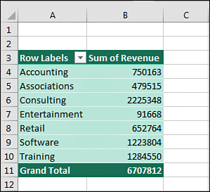
Figure 10.6 Without doing a VLOOKUP, you’ve successfully joined data from two tables in this report.
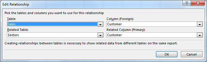
If the Auto-Detect relationship fails, use Data, Relationships, Edit Relationship. Choose Sales as the first table and Customer as the column. Choose Sectors as the second table and Customer as the related column (see Figure 10.7).
Tell Me Again—Why Is This Better Than Doing a VLOOKUP?
If you don’t have the Power Pivot add-in, you may not be convinced that all of the hassle in the preceding section is worthwhile. You now have the ability to do some cool tricks that you could never do in a regular pivot-cache pivot table. The following case study provides some examples.
Case Study: Showing Top Customer but Total Revenue
The Top 10 filter in regular pivot tables lets you show the top N customers, but you cannot get a true total of all records. Now that your data is in the Data Model, you can do this easily.
Starting with the pivot table in Figure 10.8, which shows Sector and Revenue, perform these steps:
1. Choose Customer from the Sales table in the PivotTable Fields list. Customer becomes the inner row field.
2. Open the Row Labels drop-down in cell A3. Open the Select Field drop-down and choose Customer.
3. Choose Value Filters and then Top 10.
4. In the Top 10 dialog, select Top 1 Items by Sum of Revenue. The pivot table now shows one customer per sector. As you can see in Figure 10.8, the grand total is only $3.96 million instead of the $6.7 million shown previously in Figure 10.6.
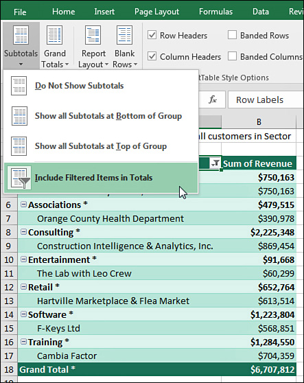
5. On the Design tab, open the Subtotals drop-down. Choose Include Filtered Items in Totals (see Figure 10.9). Each total is now marked with an asterisk, and the totals include all customers, not just the customers shown.
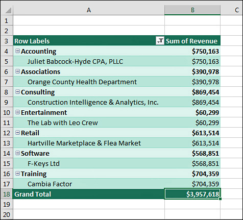
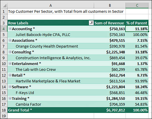
The report in Figure 10.9 is the type of report managers would like to see. It doesn’t show hundreds of customers but would let the managers talk intelligently about who is the leading customer in each sector.
In fact, a manager just called and asked for the change shown in Figure 10.10. Therefore, add Revenue to the report a second time. Choose the second Revenue heading. Choose Field Settings. Change the calculation to Percent of Parent Row Total. You now have a report showing that Cambia Factor is 54.83% of the Training sector and that the Training sector is 19.15% of the total.
Creating a New Pivot Table from an Existing Data Model
As you go from example to example in this book, it is easy to delete the pivot table sheet and start over with a fresh pivot table. It is slightly more complicated to start over after you already have data in the Data Model. But you can do it by following these simple steps:
1. While in a blank cell in the grid, choose Insert, PivotTable.
2. In the Create Pivot Table dialog, choose Use This Workbook’s Data Model.
Getting a Distinct Count
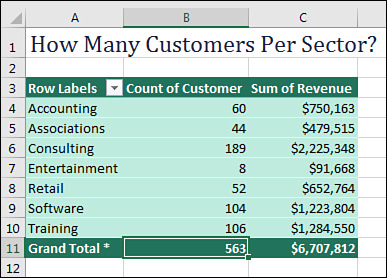
Excel pivot tables can count text values. The pivot table in Figure 10.11 is typical: Sector in the Rows area, Customer and Revenue in the Values area. You get a report showing that there are 563 customers. This is, of course, incorrect. There were 563 records that had nonblank customer names, but there were not 563 different customers. This is an ugly limitation of pivot tables that we have lived with.
If your pivot table is based on the Data Model, you can get a distinct count by following these steps:
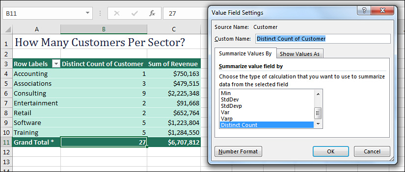
1. Go to the Customer field at the bottom of the PivotTable Fields list. Open the drop-down and choose Value Field Settings. You now see the Value Field Settings dialog, where you could normally choose Sum, Average, Count, and so on.
2. Scroll to the bottom of the list in the Value Field Settings dialog. Along the way, you might or might not notice that Product and Index are missing from the list. Any sorrow over their loss will quickly be erased when you find a new item at the bottom called Distinct Count. Choose this and click OK.
3. The pivot table now shows that there are actually 27 unique customers in the database, 9 of which are in the consulting sector (see Figure 10.12).
If I had a dollar for every time I needed a Distinct Count command in the past 10 years, I would easily have enough to afford the upgrade to Office Pro Plus. Speaking of that, the following section contrasts how to build a model if you are using the Power Pivot add-in.
Using the Power Pivot Add-in Excel 2016 Pro Plus
If your version of Excel 2016 includes the full Power Pivot add-in, you receive several benefits:
![]() You have more ways to get data into Power Pivot—more data sources, plus linked tables, copy and paste, and feeds.
You have more ways to get data into Power Pivot—more data sources, plus linked tables, copy and paste, and feeds.
![]() You can view, sort, and filter data in the Power Pivot grid.
You can view, sort, and filter data in the Power Pivot grid.
![]() You can import many millions of rows into a single worksheet in the Power Pivot grid.
You can import many millions of rows into a single worksheet in the Power Pivot grid.
![]() You can use DAX formula calculations both in the grid and as new calculated fields called measures. DAX, which stands for Data Analysis Expressions and is discussed later in this chapter, is composed of 135 functions that let you to do two types of calculations. There are 81 typical Excel functions that you can use to add a calculated column to a table in the PowerPoint window. Then you can use 54 functions to create a new measure in the pivot table. These 54 functions add incredible power to pivot tables.
You can use DAX formula calculations both in the grid and as new calculated fields called measures. DAX, which stands for Data Analysis Expressions and is discussed later in this chapter, is composed of 135 functions that let you to do two types of calculations. There are 81 typical Excel functions that you can use to add a calculated column to a table in the PowerPoint window. Then you can use 54 functions to create a new measure in the pivot table. These 54 functions add incredible power to pivot tables.
![]() You have more ways to create relationships, including a Diagram view to show relationships.
You have more ways to create relationships, including a Diagram view to show relationships.
![]() You can hide or rename columns.
You can hide or rename columns.
![]() You can set the numeric formatting for a column before you create a pivot table.
You can set the numeric formatting for a column before you create a pivot table.
![]() You can assign categories such as Geography, Image URL, and Web URL to fields.
You can assign categories such as Geography, Image URL, and Web URL to fields.
![]() You can define key performance indicators or hierarchies.
You can define key performance indicators or hierarchies.
Note
If you plan to deal with millions of records, you should opt for the 64-bit versions of Office and Power Pivot. With those versions, you are still constrained by available memory, but because Power Pivot can compress data, you can fit 10 times that amount of data in a Power Pivot file. The 64-bit version of Office can make use of memory sizes beyond the 4GB limit in 32-bit Windows.
Enabling Power Pivot
If you have Office 365 Pro Plus, Office 2016 Pro Plus, Office 2016 Enterprise, or a stand-alone boxed version of Excel 2016, you probably have Power Pivot. With one of these versions, enable Power Pivot by following these steps:
1. Open Excel 2016. Do you see a Power Pivot tab in the ribbon? If so, you can skip the remaining steps.
2. Select File, Options and choose Add-ins from the left column. At the bottom, choose Manage: COM Add-ins. Click Go.
3. Look for Microsoft Office Power Pivot for Excel 2016 in the list of available COM add-ins. Check the box next to this option and click OK.
4. If the Power Pivot tab does not appear in the ribbon, close Excel 2016 and then restart it.
The next sections walk you through your first Power Pivot data mash-up. You’ll create a report that merges a 1.8 million–row CSV file with a store identifying data in Excel.
Importing a Text File Using Power Query
Your main table in this example is a 1.8 million–record CSV file called 10-BigData.txt. It is important that you have column headings in row 1 of the CSV file. The file includes a StoreID field, but of course there are not 1.8 million store names, regions, and so on.
Create a workbook that has a StoreName lookup table. You will load the 1.8 million rows into this workbook.
Note
After Microsoft introduced the highly successful Power Query tool for Excel 2010 and Excel 2013, someone in marketing decided that the word Power in Power Query is too intimidating and started calling this feature Get and Transform. I am simply refusing to acknowledge the de-branding of this awesome feature. Throughout this chapter, I continue to refer to it as Power Query.
To import the 1.8 million–row file into Power Pivot, follow these steps:
1. Choose Data, New Query, From File, From CSV.
2. Browse to find your file. You will have to change Files of Type from CSV to All Files since your extension is .txt.
3. If you need to do any transformations using Power Query, make those changes.
4. On the Home tab of Power Query, open the Close and Load drop-down. Choose Close and Load To.
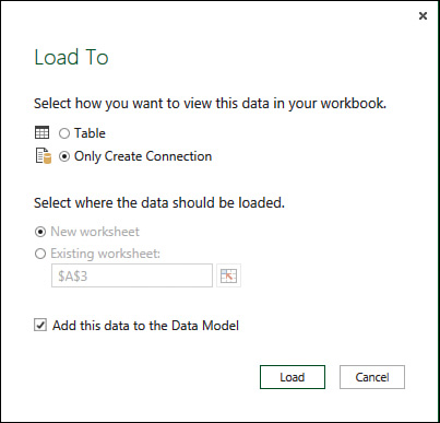
5. In the Load To pane, shown in Figure 10.13, choose Only Create Connection and check Add This Data to the Data Model. Click OK.
If you want to browse the 1.8 million rows of data, select Power Pivot, Manage. You are presented with a grid where you can scroll, sort, and filter the 1.8 million rows.
Note
Although this feels like Excel, it is not Excel. You cannot edit an individual cell. If you add a calculation in what amounts to cell E1, that calculation is automatically copied to all rows. If you format the revenue in one cell, all the cells in that column get formatted. You can change column widths by dragging the border between the column names just as in Excel.
The bottom line is that you have 1.8 million records you can sort, filter, and—later—pivot. This is going to be cool. Note that the entire 1.8 million rows from the text file are now stored in the Excel workbook. You can copy that one .xlsx file, move it to a new computer, and all of the rows will be there. You wouldn’t believe this is happening when you look at the files in Windows Explorer. The original text file is 58MB, but the Excel file is only 4MB (because of the vertical compression).
Adding Excel Data by Linking
Although you can copy Excel data and paste in Power Pivot, it is not recommended. You should link the Excel data to Power Pivot. That way, if you change the data in Excel, a simple Refresh will get the changes into Power Pivot. You need to add the StoreInfo table to the Data Model. Here’s how you do it:
1. If you start with an Excel worksheet, make sure you have single-row headings at the top, with no blank rows or blank columns.
2. Select one cell in the worksheet and press Ctrl+T. Excel asks you to confirm the extent of your table and whether your data has headers.
3. Go to the Table Tools Design tab. On the left side of the ribbon, you see that this table is called Table1. Type a new name, such as StoreInfo.
4. On the Power Pivot tab, in the Tables group, find the icon that says Add to Data Model. When you hover over it, the tooltip says that this icon will create a linked table. Click this icon to have a copy of the table appear in the Power Pivot grid.
Defining Relationships
Normally, in regular Excel you would be creating VLOOKUPs to match the two tables. Matching the tables is far easier in Power Pivot. Follow these steps:
1. In the Power Pivot window, go to the Home tab and choose Diagram View. Power Pivot shows your two tables, side by side.
2. Click the StoreID field in the main table and drag to the Store field in the lookup table. Excel draws arrows indicating the relationship (see Figure 10.14).
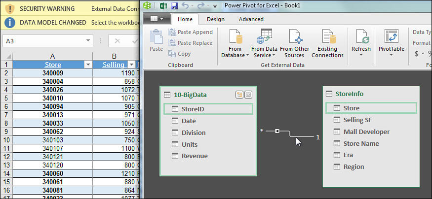
3. To return to the grid, click the Data View icon in the Home tab of the Power Pivot window.
Adding Calculated Columns Using DAX
You can add formulas in the Power Pivot grid. One common metric for retail stores is Sales per Square Foot. To enable this calculation, follow these steps:
1. Click the first worksheet tab at the bottom of the Power Pivot window. This is your 1.8 million–row data set.
2. Click in the first cell of the blank column to the right of Revenue, which has the heading Add Column.
3. Type an equal sign. Click on the Revenue column. The formula =[Revenue] appears in the formula bar.
4. Type a slash to denote division.
5. Start to type RELATED. Once it becomes the first item in AutoComplete, press Tab. (Note that RELATED is similar to VLOOKUP but far easier.)
6. AutoComplete now offers all the fields in the StoreInfo table. Double-click StoreInfo[Selling SF]. Type the final closing parenthesis. Press Enter. Excel fills the column with the calculation.
7. Right-click the column and select Rename Column. Type a name such as SalesPerSF.
At this point, you might be thinking of adding many more columns, but let’s move on to using the pivot table.
Building a Pivot Table
Open the PivotTable drop-down on the Home tab of the Power Pivot ribbon. You have choices for a single pivot table, a single chart, a chart and a table, two charts, Power View, and so on. Follow these steps:
1. Select PivotTable. You now see the Power Pivot tab back in the Excel window.
2. Select to put the pivot table on a new worksheet and click OK. You are now back in Excel. The PivotTable Fields list shows both tables, although you have to use the triangle symbol next to each table to see the fields in the table.
3. Expand the 10-BigData table in the Power Pivot Fields list and select Revenue. Expand the StoreInfo table and select Region. Excel builds a pivot table that shows sales by region (see Figure 10.15). You now have a pivot table from 1.8 million rows of data with a virtual link to a lookup table.
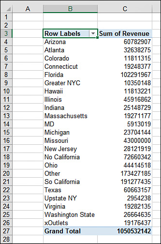
At this point, you might want to go to the PivotTable Tools tabs to further format the pivot table. You could apply a currency format and rename the Sum of Revenue field. You could also choose a format with banded rows and apply other formatting.
Understanding Differences Between Power Pivot and Regular Pivot Tables
If you have spent your whole Excel life building pivot tables out of regular Excel data, you are going to find some annoyances with Power Pivot pivot tables. Many of these issues are not because of Power Pivot. They are because any Power Pivot pivot table automatically is an OLAP pivot table. This means that it behaves like an OLAP pivot table.
Note the following differences between Power Pivot and regular pivot tables:
![]() Days of the week do not automatically sort into the proper sequencein Power Pivot. You have to choose More Sort Options, Ascending, More Options. Uncheck the AutoSort box. Open the First Key Sort Order drop-down and choose Sunday, Monday, Tuesday. Later in this chapter, you’ll see how to solve this with a Calendar table.
Days of the week do not automatically sort into the proper sequencein Power Pivot. You have to choose More Sort Options, Ascending, More Options. Uncheck the AutoSort box. Open the First Key Sort Order drop-down and choose Sunday, Monday, Tuesday. Later in this chapter, you’ll see how to solve this with a Calendar table.
![]() There is a trick in regular Excel pivot tables that you can do instead of dragging field names where you want them. Say that you go to a cell that contains the word Friday and type Monday there. When you press Enter, the Monday data moves to that new column. This does not work in Power Pivot pivot tables!
There is a trick in regular Excel pivot tables that you can do instead of dragging field names where you want them. Say that you go to a cell that contains the word Friday and type Monday there. When you press Enter, the Monday data moves to that new column. This does not work in Power Pivot pivot tables!
![]() When you enter a formula in the Excel interface, you can point to a cell to include that cell in the formula. You can do this by using the mouse or the arrow keys. Apparently, the Power Pivot team is made up of mouse people because they support building a formula using the mouse in the Power Pivot grid. Old-time Lotus 1-2-3 customers who build their formulas using arrow keys will be disappointed to find that the arrow-key method doesn’t work.
When you enter a formula in the Excel interface, you can point to a cell to include that cell in the formula. You can do this by using the mouse or the arrow keys. Apparently, the Power Pivot team is made up of mouse people because they support building a formula using the mouse in the Power Pivot grid. Old-time Lotus 1-2-3 customers who build their formulas using arrow keys will be disappointed to find that the arrow-key method doesn’t work.
![]() The Refresh button on the Analyze tab forces Excel to update the data in the pivot table. Think before you do this in Excel 2016. In the current example, this forces Excel to go out and import the 1.8 million–row data set again.
The Refresh button on the Analyze tab forces Excel to update the data in the pivot table. Think before you do this in Excel 2016. In the current example, this forces Excel to go out and import the 1.8 million–row data set again.
Using DAX Calculations
Data Analysis Expressions is a relatively new formula language. In this chapter you’ve already seen an example of using a DAX function to add a calculated column to a table in the Power Pivot grid. The 81 DAX functions are mostly copied straight from Excel for doing these types of calculations. Most of the functions are identical to their Excel counterparts, with a few exceptions listed in the next section.
You can also use DAX to create new calculated fields in a pivot table. These functions do not calculate a single cell value. They are all aggregate functions that calculate a value for the filtered rows behind any cell in the pivot table. DAX offers 54 functions to enable these calculations. The real power is in these functions.
Using DAX Calculations for Calculated Columns
You’ve already seen one example of a calculated column. The DAX functions for calculated columns are remarkably similar to the same functions in Excel, and mostly don’t require a lot of explanation. However, there are a few oddities where Excel functions were renamed in DAX:
![]() The rarely documented
The rarely documented DATEDIF function in Excel has been renamed YEARFRAC and was rewritten to actually work.
![]() The
The TEXT function in Excel was renamed FORMAT.
![]() The
The SUMIFS function was replaced and enhanced by CALCULATE.
![]() The
The VLOOKUP function was simplified with the RELATED function.
![]() DAX introduced the
DAX introduced the BLANK function. Because some of the aggregation functions can base a calculation on either ALLNONBLANKROW or FIRSTNONBLANK, you can use the BLANK function in an IF function to exclude certain rows from measure calculations.
![]() The
The CHOOSE function was renamed SWITCH. Also, whereas CHOOSE must work with values from 1 to 255, the SWITCH function can be programmed to work with other values.
Using DAX to Create a Calculated Field in a Pivot Table
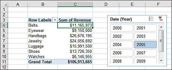
DAX calculated fields can run circles around traditional calculated fields. They are calculated only once per cell in the resultant pivot table. In Figure 10.16, the pivot table has numeric values in C4:C11. If you define a new DAX calculated field, it is calculated only for the 8 numeric cells in the pivot table. This is a lot faster than calculating 1.8 million cells and then summarizing. Before building your first calculated field, you need to understand filters, discussed next.
Filtering with DAX Calculated Fields
As you start to use DAX calculated fields, you have to realize that calculated fields automatically respect all filters applied to any particular cell in the pivot table. DAX filters first and then calculates. To understand this, consider cell C4 in Figure 10.16.
Think about how many filters are applied to cell C4. Would you say one? I think that the answer is two.
Everyone would agree that slicers are filtering the cell. Cell C4 is filtered to show only records that fall in the year 2005, based on the first slicer. That is one filter.
In addition, the Belts row header in B4 is really filtering C4 to include only records in the Belts division. That is the second filter.
Note
With DAX calculated fields, remember that to figure out the value for a particular cell in the pivot table, the calculation engine first filters and then calculates the result by using the DAX formula.
Defining a DAX Calculated Field
To define a new calculated field, go to the Excel ribbon, click the Power Pivot tab, and choose Measures, New Measure.
Microsoft used the term measures in Excel 2010 and then switched to calculated fields in Excel 2013. As this book goes to press, Microsoft has returned to calling them measures, but do not be surprised if it returns to using calculated fields in some future monthly release of Office 365.
You should specify your main table in the Table Name box. Give it a name like StoreCount. Type your formula in the formula box and use the fx icon to insert function names. For field names, start by typing a few characters of the table name and then use the AutoComplete list to select the field.
When you are done, click the Check Formula button to check the syntax. Note that the tooltip for the function still covers up the result of the Check Formula command. Click in the Description field to hide the tooltip so you can see the result of the Check Formula command. You should see “No errors in formula,” as shown in Figure 10.17.
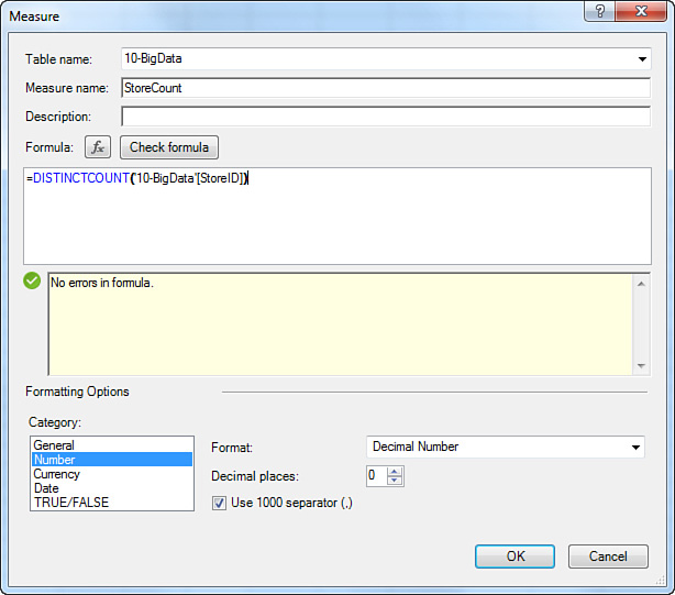
Click OK to add the new calculated field to the PivotTable Fields list.
After you define a calculated field, you can use that field in future calculations. The SalesPerStore field in Figure 10.18 is calculated as =[Sum of Revenue]/ [StoreCount].
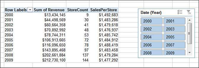
Figure 10.18 SalesPerStore is calculated from a field in the data divided by a different DAX calculated field.
You do not have to display Sum of Revenue or StoreCount in the pivot table. You could simplify the pivot table to show only SalesPerStore.
Using Time Intelligence
Typically, Excel stores dates as a serial number. When you enter 2/17/2018 in a cell, Excel only knows that this date is 43,148 days after December 31, 1899. Power Pivot adds time intelligence. When you have a date such as 2/17/2018 in Power Pivot, there are time intelligence functions that know that year-to-date means 1/1/2018 through 2/17/2018. The time intelligence functions know that month-to-date from the prior year is 2/1/2017 through 2/17/2017.
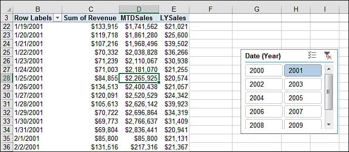
Remember that each value cell in a pivot table is a result of filters imposed by the slicers and by the row and column fields. Cell D28 in Figure 10.19 is being filtered to 2001 by the slicer and further filtered to January 25, 2001, by the row field in B28. But that cell needs to break free of the filter in order to add all of the sales from January 1, 2001, through January 25, 2001. The CALCULATE function helps you solve this problem.
In many ways, the DAX CALCULATE function is like a super-human version of the Excel SUMIFS function. =CALCULATE(Field,Filter,Filter,Filter,Filter) is the syntax. But any Filter argument could actually unapply a filter that’s being imposed by a slicer or a row field.
DATESMTD([Date]) returns all of the dates used to calculate the month-to-date total for the cell. For January 25, 2001, the DATESMTD function will return January 1 through 25, 2001. When you use DATESMTD as the filter in the CALCULATE function, it breaks the chains of the 1/25/2001 filter and reapplies a new filter of January 1–25, 2001. The DAX formula for MTDSales is
=CALCULATE([Sum of Revenue],DATESMTD('10-BigData'[Date]))
The measure in column E requires two filter arguments. First, you need to tell DAX to ignore the Years filter. Use ALL([Years]) to do this. Then, you need to point to one year ago. Use DATEADD([Date],-1,YEAR) to move backward one year from January 25, 2002, to January 25, 2001. Therefore, this is the formula for LYSales:
CALCULATE([Sum of Revenue],
All('10-BigData'[Date (Year)]),
DATEADD('10-BigData'[Date],-1,YEAR))
Other time intelligence functions include DATESQTD and DATESYTD.
Note
To learn more about DAX, read DAX Formulas for Power Pivot, Second Edition, by Rob Collie and Avi Singh.
Next Steps
While Power Pivot lets you build pivot tables from complex models, the new Power View add-in for Excel 2016 Pro Plus customers lets you combine multiple Power Pivot charts in an animated, interactive dashboard within Excel. The 3D Map feature lets you animate your data on a globe. Chapter 11 introduces Power View and 3D Map.