9. Working with and Analyzing OLAP Data
In This Chapter
Understanding the Structure of an OLAP Cube
Understanding the Limitations of OLAP Pivot Tables
Breaking Out of the Pivot Table Mold with Cube Functions
Adding Calculations to OLAP Pivot Tables
Introduction to OLAP
Online analytical processing (OLAP) is a category of data warehousing that enables you to mine and analyze vast amounts of data with ease and efficiency. Unlike other types of databases, OLAP databases are designed specifically for reporting and data mining. In fact, there are several key differences between standard transactional databases, such as Access and SQL Server, and OLAP databases.
Records within a transactional database are routinely added, deleted, and updated. OLAP databases, on the other hand, contain only snapshots of data. The data in an OLAP database is typically archived data, stored solely for reporting purposes. Although new data may be appended on a regular basis, existing data is rarely edited or deleted.
Another difference between transactional databases and OLAP databases is structure. Transactional databases typically contain many tables; each table usually contains multiple relationships with other tables. Indeed, some transactional databases contain so many tables that it can be difficult to determine how each table relates to another.
In an OLAP database, however, all the relationships between the various data points have been predefined and stored in OLAP cubes. These cubes already contain the relationships and hierarchies you need to easily navigate the data within. Consequently, you can build reports without needing to know how the data tables relate to one another.
The biggest difference between OLAP and transactional databases is the way the data is stored. The data in an OLAP cube is rarely stored in raw form. OLAP cubes typically store data in views that are already organized and aggregated. That is, grouping, sorting, and aggregations are predefined and ready to use. This makes querying and browsing for data far more efficient than in a transactional database, where you have to group, aggregate, and sort records on the fly.
Note
An OLAP database is typically set up and maintained by the database administrator in your IT department. If your organization does not utilize OLAP databases, you might want to speak with your database administrator about the possibility of using some OLAP reporting solutions.
Connecting to an OLAP Cube
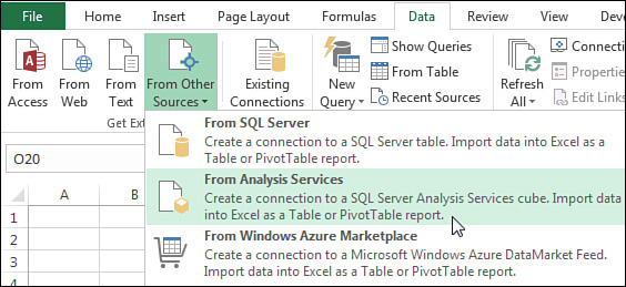
Before you can browse OLAP data, you must establish a connection to an OLAP cube. Start on the Data tab and select From Other Sources to see the drop-down menu shown in Figure 9.1. Then select the From Analysis Services option.
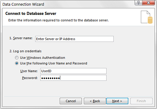
Selecting this option activates the Data Connection Wizard, shown in Figure 9.2. The idea here is that you configure your connection settings so Excel can establish a link to the server. Here are the steps to follow:
Note
The examples in this chapter have been created using the Analysis Services Tutorial cube that comes with SQL Server Analysis Services 2012. The actions you take to connect to and work with your OLAP database are the same as demonstrated here because the concepts are applicable to any OLAP cube you are using.
1. Provide Excel with authentication information. Enter the name of your server as well as your username and password, as demonstrated in Figure 9.2. Then click Next.
Note
If you are typically authenticated via Windows Authentication, you simply select the Use Windows Authentication option.
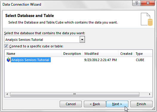
2. Select the database with which you are working from the drop-down box. As Figure 9.3 illustrates, the Analysis Services Tutorial database is selected for this scenario. Selecting this database causes all the available OLAP cubes to be exposed in the list of objects below the drop-down menu. Choose the cube you want to analyze and then click Next.
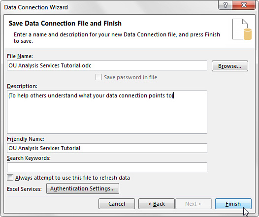
3. On the next screen, shown in Figure 9.4, enter some descriptive information about the connection you’ve just created.
Note
All the fields in the screen shown in Figure 9.4 are optional. That is, you can bypass this screen without editing anything, and your connection will work fine.
4. Click the Finish button to finalize your connection settings. You immediately see the Import Data dialog, as shown in Figure 9.5.
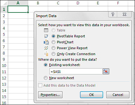
5. In the Import Data dialog, select PivotTable Report and then click the OK button to start building your pivot table.
Understanding the Structure of an OLAP Cube
When a pivot table is created, you might notice that the PivotTable Fields list looks somewhat different from that of a standard pivot table. The reason is that the PivotTable Fields list for an OLAP pivot table is arranged to represent the structure of the OLAP cube you are connected to.
To effectively browse an OLAP cube, you need to understand the component parts of OLAP cubes and the way they interact with one another. Figure 9.6 illustrates the basic structure of a typical OLAP cube.
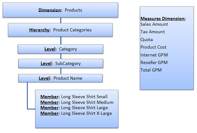
As you can see, the main components of an OLAP cube are dimensions, hierarchies, levels, members, and measures:
![]() Dimensions—Major classifications of data that contain the data items that are analyzed. Some common examples of dimensions are the Products dimension, Customer dimension, and Employee dimension. The structure shown in Figure 9.6 is the Products dimension.
Dimensions—Major classifications of data that contain the data items that are analyzed. Some common examples of dimensions are the Products dimension, Customer dimension, and Employee dimension. The structure shown in Figure 9.6 is the Products dimension.
![]() Hierarchies—Predefined aggregations of levels within a particular dimension. A hierarchy enables you to pivot and analyze multiple levels at one time without having any knowledge of the relationships between the levels. In the example in Figure 9.6, the Products dimension has three levels that are aggregated into one hierarchy called Product Categories.
Hierarchies—Predefined aggregations of levels within a particular dimension. A hierarchy enables you to pivot and analyze multiple levels at one time without having any knowledge of the relationships between the levels. In the example in Figure 9.6, the Products dimension has three levels that are aggregated into one hierarchy called Product Categories.
![]() Levels—Categories of data that are aggregated within a hierarchy. You can think of levels as data fields that can be queried and analyzed individually. In Figure 9.6, note that there are three levels: Category, Subcategory, and Product Name.
Levels—Categories of data that are aggregated within a hierarchy. You can think of levels as data fields that can be queried and analyzed individually. In Figure 9.6, note that there are three levels: Category, Subcategory, and Product Name.
![]() Members—The individual data items within a dimension. Members are typically accessed via the OLAP structure of dimension, hierarchy, level, and member. In the example shown in Figure 9.6, the members you see belong to the Product Name level. The other levels have their own members and are not shown here.
Members—The individual data items within a dimension. Members are typically accessed via the OLAP structure of dimension, hierarchy, level, and member. In the example shown in Figure 9.6, the members you see belong to the Product Name level. The other levels have their own members and are not shown here.
![]() Measures—The data values within the OLAP cube. Measures are stored within their own dimension, appropriately called the Measures dimension. The idea is that you can use any combination of dimension, hierarchy, level, and member to query the measures. This is called slicing the measures.
Measures—The data values within the OLAP cube. Measures are stored within their own dimension, appropriately called the Measures dimension. The idea is that you can use any combination of dimension, hierarchy, level, and member to query the measures. This is called slicing the measures.
Now that you understand how the data in an OLAP cube is structured, take a look at the PivotTable Fields list in Figure 9.7, and the arrangement of the available fields should begin to make sense.
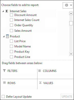
As you can see, the measures are listed first under the Sigma icon. These are the only items you can drop in the Values area of the pivot table. Next, you see dimensions represented next to the table icon. In this example, you see the Product dimension. Under the Product dimension, you see the Product Categories hierarchy that can be drilled into. Drilling into the Product Categories hierarchy enables you to see the individual levels.
The cool thing is that you are able to browse the entire cube structure by simply navigating through your PivotTable Fields list! From here, you can build your OLAP pivot table report just as you would build a standard pivot table.
Understanding the Limitations of OLAP Pivot Tables
When working with OLAP pivot tables, you must remember that the source data is maintained and controlled in the Analysis Services OLAP environment. This means that every aspect of the cube’s behavior—from the dimensions and measures included in the cube to the ability to drill into the details of a dimension—is controlled via Analysis Services. This reality translates into some limitations on the actions you can take with your OLAP pivot tables.
When your pivot table report is based on an OLAP data source, keep in mind the following:
![]() You cannot place any field other than measures into the Values area of the pivot table.
You cannot place any field other than measures into the Values area of the pivot table.
![]() You cannot change the function used to summarize a data field.
You cannot change the function used to summarize a data field.
![]() The Show Report Filter Pages command is disabled.
The Show Report Filter Pages command is disabled.
![]() The Show Items with No Data option is disabled.
The Show Items with No Data option is disabled.
![]() The Subtotal Hidden Page Items setting is disabled.
The Subtotal Hidden Page Items setting is disabled.
![]() The Background Query option is not available.
The Background Query option is not available.
![]() Double-clicking in the Values field returns only the first 1,000 records of the pivot cache.
Double-clicking in the Values field returns only the first 1,000 records of the pivot cache.
![]() The Optimize Memory check box in the PivotTable Options dialog is disabled.
The Optimize Memory check box in the PivotTable Options dialog is disabled.
Creating an Offline Cube
With a standard pivot table, the source data is typically stored on your local drive. This way, you can work with and analyze your data while you’re disconnected from the network. However, this is not the case with OLAP pivot tables. With an OLAP pivot table, the pivot cache is never brought to your local drive. This means that while you are disconnected from the network, your pivot table is out of commission. You can’t even move a field while disconnected.
If you need to analyze your OLAP data while disconnected from your network, you need to create an offline cube. An offline cube is essentially a file that acts as a pivot cache, locally storing OLAP data so that you can browse that data while disconnected from the network.
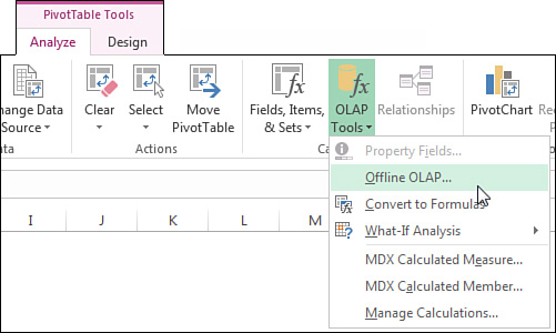
To create an offline cube, start with an OLAP-based pivot table. Place your cursor anywhere inside the pivot table and click the OLAP Tools drop-down menu button on the PivotTable Tools Analyze tab. Then select Offline OLAP, as shown in Figure 9.8.
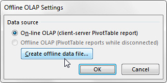
Selecting this option activates the Offline OLAP Settings dialog (see Figure 9.9), where you click the Create Offline Data File button. The Create Cube File wizard, shown in Figure 9.10, appears. Click Next to start the process.
As you can see in Figure 9.10, you first select the dimensions and levels you want included in your offline cube. Your selections tell Excel which data you want to import from the OLAP database. The idea is to select only the dimensions that you need available to you while you’re disconnected from the server. The more dimensions you select, the more disk space your offline cube file takes up.

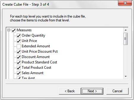
Clicking Next moves you to the next dialog, shown in Figure 9.11. Here, you are given the opportunity to filter out any members or data items you do not want included. For instance, the Extended Amount measure is not needed, so the check has been removed from its selection box. Deselecting this box ensures that this measure will not be imported and therefore will not take up unnecessary disk space.
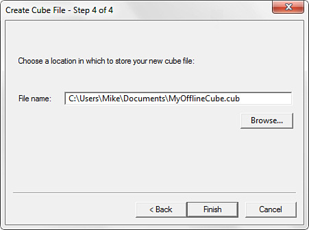
The final step is to specify a name and location for your cube file. In Figure 9.12, the cube file is named MyOfflineCube.cub, and it will be placed in a directory called Documents.
Note
The filename extension for all offline cubes is .cub.
After a few moments of crunching, Excel outputs your offline cube file to your chosen directory. To test it, simply double-click the file to automatically generate an Excel workbook that is linked to the offline cube via a pivot table.
After your offline cube file has been created, you can distribute it to others and use it while disconnected from the network.
Tip
When you’re connected to the network, you can open your offline cube file and refresh the pivot table within. This automatically refreshes the data in the cube file. The idea is that you can use the data within the cube file while you are disconnected from the network and can refresh the cube file while a data connection is available. Any attempt to refresh an offline cube while disconnected causes an error.
Breaking Out of the Pivot Table Mold with Cube Functions
Cube functions are Excel functions that can be used to access OLAP data outside a pivot table object. In pre-2010 versions of Excel, you could find cube functions only if you installed the Analysis Services add-in. In Excel 2010, cube functions were brought into the native Excel environment. To fully understand the benefit of cube functions, take a moment to walk through an example.
Exploring Cube Functions
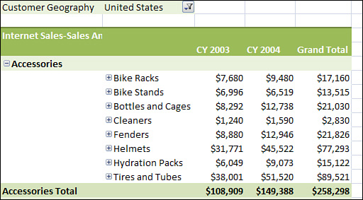
One of the easiest ways to start exploring cube functions is to allow Excel to convert your OLAP-based pivot table into cube formulas. Converting a pivot table to cube formulas is a delightfully easy way to create a few cube formulas without doing any of the work yourself. The idea is to tell Excel to replace all cells in the pivot table with a formula that connects to the OLAP database. Figure 9.13 shows a pivot table connected to an OLAP database.
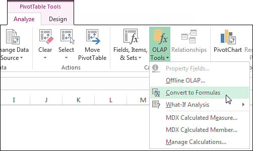
With just a few clicks, you can convert any OLAP pivot table into a series of cube formulas. Place the cursor anywhere inside the pivot table and click the OLAP Tools drop-down menu button on the PivotTable Tools Analyze tab. Select Convert to Formulas, as shown in Figure 9.14.
If your pivot table contains a report filter field, the dialog shown in Figure 9.15 appears. This dialog gives you the option of converting your filter drop-down selectors to cube formulas. If you select this option, the drop-down selectors are removed, leaving a static formula. If you need to have your filter drop-down selectors intact so that you can continue to interactively change the selections in the filter field, leave the Convert Report Filters option unchecked.

Note
If you are working with a pivot table in Compatibility mode, Excel automatically converts the filter fields to formulas.
After a second or two, the cells that used to house a pivot table are now homes for cube formulas. Note that, as shown in Figure 9.16, any styles you have applied are removed.
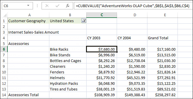
So why is this capability useful? Well, now that the values you see are no longer part of a pivot table object, you can insert rows and columns, you can add your own calculations, you can combine the data with other external data, and you can modify the report in all sorts of ways by simply moving the formulas around.
Adding Calculations to OLAP Pivot Tables
In Excel 2010 and earlier, OLAP pivot tables were limited in that you could not build your own calculations within OLAP pivot tables. This means you could not add the extra layer of analysis provided by the calculated fields and calculated items functionality in standard pivot tables.
Note
Calculated fields and calculated items are covered in Chapter 5, “Performing Calculations in Pivot Tables.” If you haven’t read it already, you might find it helpful to read that chapter first in order to build the foundation for this section.
Excel 2013 changed that with the introduction of the new OLAP tools—calculated measures and calculated members. With these two tools, you are no longer limited to just using the measures and members provided through the OLAP cube by the database administrator. You can add your own analysis by building your own calculations.
In this section, you’ll explore how to build your own calculated measures and calculated members.
Creating Calculated Measures
A calculated measure is essentially the OLAP version of a calculated field. When you create a calculated measure, you basically create a new data field based on some mathematical operation that uses the existing OLAP fields.
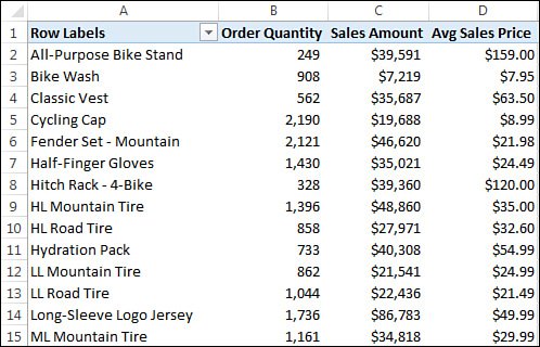
In the example shown in Figure 9.17, an OLAP pivot table contains products along with their respective quantities and revenues. Say that you want to add a new measure that calculates average sales price per unit.
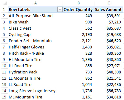
Figure 9.17 You want to add a calculation to this OLAP pivot table to show average sales price per unit.
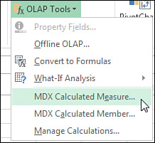
Place your cursor anywhere in the pivot table and select the PivotTable Tools Analyze tab. Then select MDX Calculated Measure, as shown in Figure 9.18. This activates the New Calculated Measure dialog, shown in Figure 9.19.

In the New Calculated Measure dialog, take the following actions:
1. Give your calculated measure a name by entering it in the Name input box.
2. Choose a measure group where Excel should place your calculated measure. If you don’t choose one, Excel automatically places your measure in the first available measure group.
3. Enter the MDX syntax for your calculation in the MDX input box. To save a little time, you can use the list on the left to choose the existing measures you need for your calculation. Simply double-click the measures needed, and Excel pops them into the MDX input box. In this example, the calculation for the average sales price is IIF([Measures].[Order Quantity] = 0,NULL,[Measures].[Sales Amount]/[Measures].[Order Quantity]).
4. Click OK.
Tip
In the New Calculated Measure dialog, shown in Figure 9.19, notice the Test MDX button. You can click this to ensure that the MDX you entered is well formed. Excel lets you know via a message box if your syntax contains any errors.
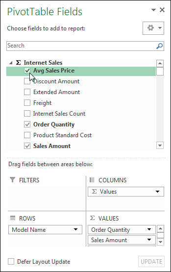
After you have built your calculated measure, you can go to the PivotTable Fields list and select your newly created calculation (see Figure 9.20).
As you can see in Figure 9.21, your calculated measure adds a meaningful layer of analysis to the pivot table.
Note
It’s important to note that when you create a calculated measure, it exists in your workbook only. In other words, you are not building your calculation directly in the OLAP cube on the server. This means no one else connected to the OLAP cube will be able to see your calculations unless you share or distribute your workbook.
Creating Calculated Members
A calculated member is essentially the OLAP version of a calculated item. When you create a calculated member, you basically create a new data item based on some mathematical operation that uses the existing OLAP members.
In the example shown in Figure 9.22, an OLAP pivot table contains sales information for each quarter in the year. Let’s say you want to aggregate quarters 1 and 2 into a new data item called First Half of Year. You also want to aggregate quarters 3 and 4 into a new data item called Second Half of Year.
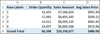
Figure 9.22 You want to add new calculated members to aggregate the four quarters into First Half of Year and Second Half of Year.
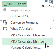
Place your cursor anywhere in the pivot table and select the PivotTable Tools Analyze tab. Then select MDX Calculated Member, as shown in Figure 9.23. The New Calculated Member dialog opens (see Figure 9.24).
In the New Calculated Member dialog, take the following actions:
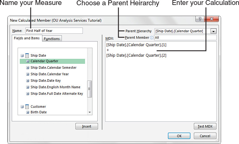
1. Give your calculated member a name by entering it in the Name input box.
2. Choose the parent hierarchy for which you are creating new members. Be sure to leave Parent Member set to All. This ensures that Excel takes into account all members in the parent hierarchy when evaluating your calculation.
3. Enter the MDX syntax for your calculation in the MDX input box. To save a little time, you can use the list on the left to choose the existing members you need for your calculation. Simply double-click the member needed, and Excel pops them into the MDX input box. In the example in Figure 9.24, you are adding quarter 1 and quarter 2: [Ship Date]·[Calendar Quarter]·[1] + [Ship Date]·[Calendar Quarter]·[2].
4. Click OK.
As soon as you click OK, Excel shows your newly created calculated member in the pivot table. As you can see in Figure 9.25, your calculated member is included with the other original members of the pivot field.
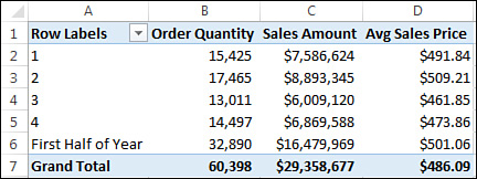
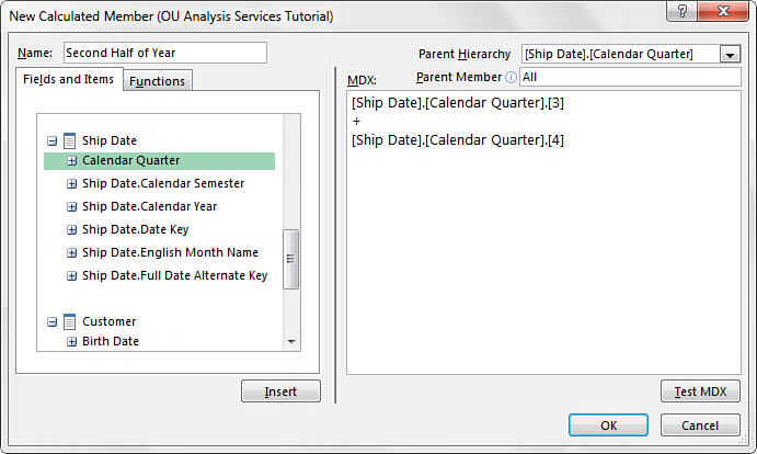
Figure 9.26 shows how you repeat the process to calculate the Second Half of Year member.
Notice in Figure 9.27 that Excel makes no attempt to remove any of the original members. In this case, you see that quarters 1 through 4 are still in the pivot table. This might be fine for your situation, but in most scenarios, you will likely hide these members to avoid confusion.
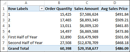
Figure 9.27 Excel shows your final calculated members along with the original members. It is a best practice to remove the original members to avoid confusion.
Note
Remember that your calculated member exists in your workbook only. No one else connected to the OLAP cube is able to see your calculations unless you share or distribute your workbook.
Caution
If the parent hierarchy or parent member is changed in the OLAP cube, your calculated member ceases to function. You must re-create the calculated member.
Managing OLAP Calculations
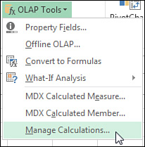
Excel provides an interface for managing the calculated measures and calculated members in an OLAP pivot table. Simply place your cursor anywhere in the pivot table and select the PivotTable Tools Analyze tab. Then select Manage Calculations, as shown in Figure 9.28.
The Manage Calculations dialog, shown in Figure 9.29, appears, offering three commands:
![]() New—Create a new calculated measure or calculated member.
New—Create a new calculated measure or calculated member.
![]() Edit—Edit the selected calculation.
Edit—Edit the selected calculation.
![]() Delete—Permanently delete the selected calculation.
Delete—Permanently delete the selected calculation.
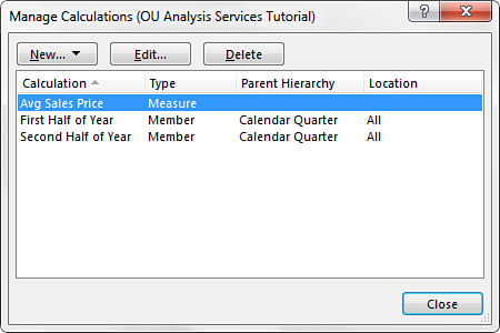
Figure 9.29 The Manage Calculations dialog enables you to create a new calculation, edit an existing calculation, or delete an existing calculation.
Performing What-If Analysis with OLAP Data
Another piece of functionality that Microsoft introduced in Excel 2013 is the ability to perform what-if analysis with the data in OLAP pivot tables. With this functionality, you have the ability to actually edit the values in a pivot table and recalculate your measures and members based on your changes. You even have the ability to publish your changes back to the OLAP cube.
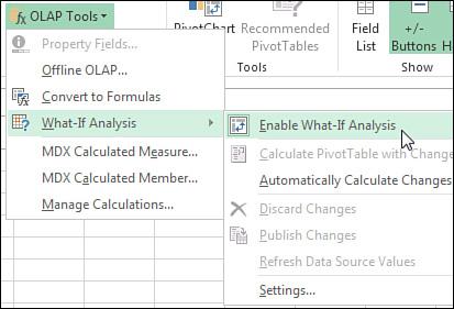
To make use of the what-if analysis functionality, create an OLAP pivot table and then go to the PivotTable Tools Analyze tab. Once there, select What-If Analysis, Enable What-If Analysis, as shown in Figure 9.30.
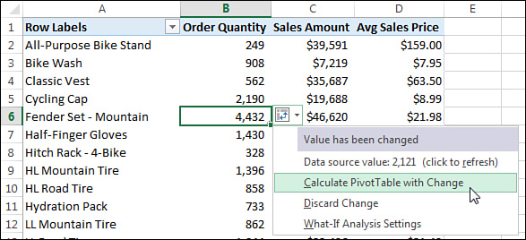
At this point, you can edit the values in your pivot table. After you have made changes, you can right-click any of the changed values and choose Calculate PivotTable with Change (see Figure 9.31). This forces Excel to reevaluate all the calculations in the pivot table based on your edits—including your calculated members and measures.
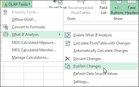
The edits you make to your pivot table while using what-if analysis are, by default, local edits only. If you are committed to your changes and would like to actually make the changes on the OLAP server, you can tell Excel to publish your changes. To do this, in the PivotTable Tools Analyze tab, select What-If Analysis, Publish Changes (see Figure 9.32). This triggers a “write-back” to the OLAP server, meaning the edited values are sent to the source OLAP cube.
Note
You need adequate server permissions to publish changes to the OLAP server. Your database administrator can guide you through the process of getting write access to your OLAP database.
Next Steps
In Chapter 10, “Mashing Up Data with Power Pivot,” you’ll find out how to use PowerPivot to create powerful reporting models that are able to process and analyze millions of rows of data in a single pivot table.