
7. Analyzing Disparate Data Sources with Pivot Tables
In This Chapter
Building a Pivot Table Using External Data Sources
Leveraging Power Query to Extract and Transform Data
Up to this point, you have been working with one local table located in the worksheet within which you are operating. Indeed, it would be wonderful if every data set you came across were neatly packed in one easy-to-use Excel table. Unfortunately, the business of data analysis does not always work out that way.
The reality is that some of the data you encounter will come from disparate data sources—sets of data that are from separate systems, stored in different locations, or saved in a variety of formats. In an Excel environment, disparate data sources generally fall into one of two categories:
![]() External data—External data is exactly what it sounds like—data that is not located in the Excel workbook in which you are operating. Some examples of external data sources are text files, Access tables, SQL Server tables, and other Excel workbooks.
External data—External data is exactly what it sounds like—data that is not located in the Excel workbook in which you are operating. Some examples of external data sources are text files, Access tables, SQL Server tables, and other Excel workbooks.
![]() Multiple ranges—Multiple ranges are separate data sets located in the same workbook but separated either by blank cells or by different worksheets. For example, if your workbook has three tables on three different worksheets, each of your data sets covers a range of cells. You are therefore working with multiple ranges.
Multiple ranges—Multiple ranges are separate data sets located in the same workbook but separated either by blank cells or by different worksheets. For example, if your workbook has three tables on three different worksheets, each of your data sets covers a range of cells. You are therefore working with multiple ranges.
A pivot table can be an effective tool when you need to summarize data that is not neatly packed into one table. With a pivot table, you can quickly bring together either data found in an external source or data found in multiple tables within your workbook. In this chapter, you’ll discover various techniques for working with external data sources and data sets located in multiple ranges within a workbook.
Using the Internal Data Model
Excel 2013 introduced a new in-memory analytics engine called the Data Model. Every workbook has one internal Data Model that enables you to work with and analyze disparate data sources like never before.
The idea behind the Data Model is simple. Let’s say you have two tables: a Customers table and an Orders table. The Orders table contains basic information about invoices (customer number, invoice date, and revenue). The Customers table contains information such as customer number, customer name, and state. If you want to analyze revenue by state, you have to join the two tables and aggregate the Revenue field in the Orders table by the State field in the Customers table.
In the past, in order to do this, you would have had to go through a series of gyrations involving using VLOOKUP, SUMIF, or other functions. With the new Data Model, however, you can simply tell Excel how the two tables are related (they both have customer number) and then pull them into the internal Data Model. The Excel Data Model then builds an analytical cube based on that customer number relationship and exposes the data through a pivot table. With the pivot table, you can create the aggregation by state with a few mouse clicks.
![]() The internal Data Model is secretly using the Power Pivot data engine. If you have Excel Pro Plus or higher, you can take the Data Model further. See Chapter 10, “Mashing Up Data with PowerPivot.”
The internal Data Model is secretly using the Power Pivot data engine. If you have Excel Pro Plus or higher, you can take the Data Model further. See Chapter 10, “Mashing Up Data with PowerPivot.”
Building Out Your First Data Model
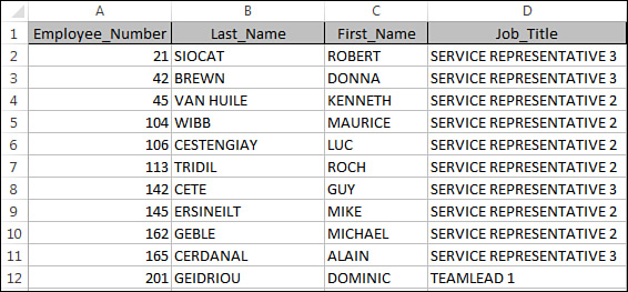
Imagine that you have the Transactions table shown in Figure 7.1. On another worksheet, you have the Employees table shown in Figure 7.2.

You need to create an analysis that shows sales by job title. This would normally be difficult, given the fact that sales and job title are in two separate tables. But with the new Data Model, you can follow these simple steps:
1. Click inside the Transactions data table and start a new pivot table (by using Insert, Pivot Table on the ribbon).
2. In the Create PivotTable dialog, be sure to place a check next to the Add This Data to the Data Model option (see Figure 7.3).

Figure 7.3 Create a new pivot table from the Transactions table. Make sure you select Add This Data to the Data Model.
3. Click inside the Employees data table and start a new pivot table. Again, be sure to place a check next to the Add This Data to the Data Model option, as demonstrated in Figure 7.4.
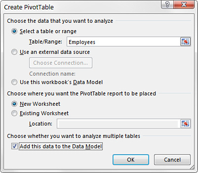
Figure 7.4 Create a new pivot table from the Employees table. Make sure to select Add This Data to the Data Model.
Note
Notice that in Figures 7.3 and 7.4, the Create PivotTable dialogs are referencing named ranges. That is to say, each table was given a specific name. When you’re adding data to the Data Model, it’s a best practice to name your data tables. This way, you can easily recognize your tables in the Data Model. If you don’t name your tables, the Data Model shows them as Range1, Range2, and so on.
To give a data table a name, simply highlight all the data in the table, select the Formulas tab on the ribbon, and then click the Define Name command. In the dialog, enter a name for the table. Repeat for all other tables.
4. Once both tables have been added to the Data Model, activate the PivotTable Fields list and choose ALL, as shown in Figure 7.5, to see both ranges in the fields list.

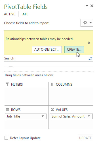
5. Build out your pivot table as normal. In this case, Job_Title goes to the Rows area and Sales_Amount goes to the Values area. As you can see in Figure 7.6, Excel immediately recognizes that you are using two tables from your Data Model and prompts you to create a relationship between them. You can let Excel auto-detect the relationships between your tables, or you can click the Create button. It’s best to create relationships yourself to avoid any possibility of Excel getting it wrong, so click the Create button.
6. Excel activates the Create Relationship dialog shown in Figure 7.7. Here, you select the tables and fields that define the relationship. In Figure 7.7, you can see that the Transactions table has a Sales_Rep field. It is related to the Employees table via the Employee_Number field.

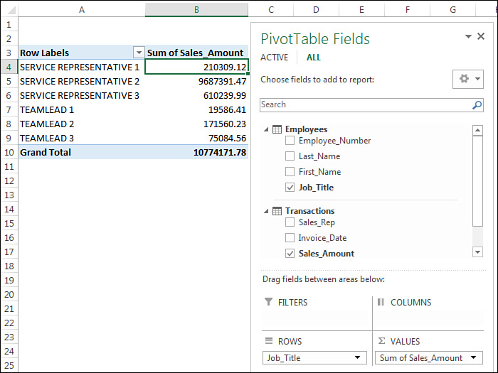
After you create the relationship, you have a single pivot table that effectively uses data from both tables to create the analysis you need. Figure 7.8 illustrates that using the Excel Data Model, you have achieved the goal of showing sales by job title.
Managing Relationships in the Data Model
After you assign tables to the internal Data Model, you might need to adjust the relationships between the tables. To make changes to the relationships in a Data Model, activate the Manage Relationships dialog.
Click the Data tab in the ribbon and select the Relationships command. The dialog shown in Figure 7.9 appears.

Figure 7.9 The Manage Relationships dialog enables you to make changes to the relationships in the Data Model.
The Manage Relationships dialog offers the following buttons:
![]() New—Create a new relationship between two tables in the Data Model.
New—Create a new relationship between two tables in the Data Model.
![]() Edit—Alter the selected relationship.
Edit—Alter the selected relationship.
![]() Activate—Enforce the selected relationship; that is, tell Excel to consider the relationship when aggregating and analyzing the data in the Data Model.
Activate—Enforce the selected relationship; that is, tell Excel to consider the relationship when aggregating and analyzing the data in the Data Model.
![]() Deactivate—Turn off the selected relationship; that is, tell Excel to ignore the relationship when aggregating and analyzing the data in the Data Model.
Deactivate—Turn off the selected relationship; that is, tell Excel to ignore the relationship when aggregating and analyzing the data in the Data Model.
![]() Delete—Remove the selected relationship.
Delete—Remove the selected relationship.
Adding a New Table to the Data Model
You can add a new table to the Data Model in one of two ways. The easiest way is to simply create a pivot table from the new table and then choose the Add This Data to the Data Model option. Excel adds your table to the Data Model and produces a pivot table. After your table has been added, you can open the Manage Relationships dialog and create the needed relationship.
The second and more flexible method is to manually define a table and add it to the Data Model. Here’s how:
1. Place your cursor inside a data table and select Insert Table. The Create Table dialog, shown in Figure 7.10, appears.
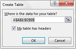
2. In the Create Table dialog, specify the range for your data. Excel turns that range into a defined table that the internal Data Model can recognize.
3. On the Table Tools Design tab, change the Table Name field (in the Properties group) to something appropriate that’s easy to remember (see Figure 7.11).

4. Go to the Data tab in the ribbon and select Connections to open the Workbook Connections dialog, shown in Figure 7.12. Click the drop-down next to Add and choose the Add to the Data Model option.

5. In the Existing Connections dialog that appears (see Figure 7.13), select the Tables tab. Then find and select your newly created table. Click the Open button to add the table to the Data Model.
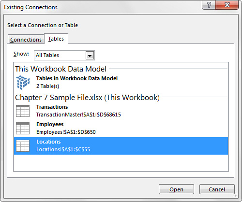
At this point, all pivot tables built on the Data Model are updated to reflect the new table. Be sure to open the Manage Relationships dialog and create the needed relationship.
Caution
Be aware that every table you add to the Data Model is essentially stored with the workbook, effectively increasing the size of your Excel file. Read more about the size limitations of the Excel Data Model later in the chapter.
Removing a Table from the Data Model
You might find that you want to remove a table or data source altogether from the Data Model. To do so, click the Data tab in the ribbon and then click Connections. The Workbook Connections dialog, shown in Figure 7.14, opens.

Click the table you want to remove from the Data Model (Employees, in this case), and then click the Remove button.
Creating a New Pivot Table Using the Data Model
There might be instances when you want to create a pivot table from scratch using the existing internal Data Model as the source data. Here are the steps to do so:
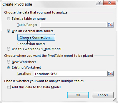
1. Activate the Create PivotTable dialog by clicking Insert, PivotTable. Click the Use an External Data Source option (see Figure 7.15). Then click the Choose Connection button.
2. In the Existing Connections dialog that appears (see Figure 7.16), select the Tables tab. Then select Tables in Workbook Data Model and click the Open button.
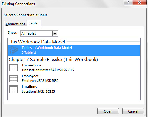
Figure 7.16 Use the Existing Connections dialog to select the internal Data Model as the data source for the pivot table.
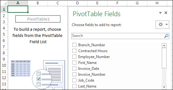
3. When Excel takes you back to the Create PivotTable dialog, click the OK button to create the pivot table. If all goes well, the PivotTable Fields list now shows all the tables that are included in the internal Data Model (see Figure 7.17).

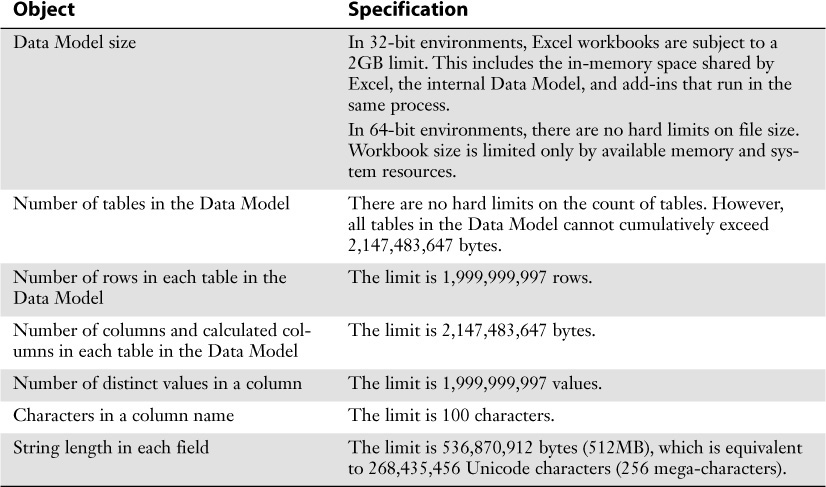
Limitations of the Internal Data Model
As with everything else in Excel, the internal Data Model does have limitations. Table 7.1 highlights the maximum and configurable limits for the Excel Data Model.
Building a Pivot Table Using External Data Sources
Excel is certainly good at processing and analyzing data. In fact, pivot tables themselves are a testament to the analytical power of Excel. However, despite all its strengths, Excel makes for a poor relational data management platform, primarily for three reasons:
![]() A data set’s size has a significant effect on performance, making for less efficient data crunching. The reason for this is the fundamental way Excel handles memory. When you open an Excel file, the entire file is loaded into RAM to ensure quick data processing and access. The drawback to this behavior is that Excel requires a great deal of RAM to process even the smallest change in a spreadsheet (and typically gives you a “Calculating” indicator in the status bar). So although Excel 2016 offers more than 1 million rows and more than 16,000 columns, creating and managing large data sets causes Excel to slow down considerably, making data analysis a painful endeavor.
A data set’s size has a significant effect on performance, making for less efficient data crunching. The reason for this is the fundamental way Excel handles memory. When you open an Excel file, the entire file is loaded into RAM to ensure quick data processing and access. The drawback to this behavior is that Excel requires a great deal of RAM to process even the smallest change in a spreadsheet (and typically gives you a “Calculating” indicator in the status bar). So although Excel 2016 offers more than 1 million rows and more than 16,000 columns, creating and managing large data sets causes Excel to slow down considerably, making data analysis a painful endeavor.
![]() The lack of a relational data structure forces the use of flat tables that promote redundant data. This also increases the chance for errors.
The lack of a relational data structure forces the use of flat tables that promote redundant data. This also increases the chance for errors.
![]() There is no way to index data fields in Excel to optimize performance when you’re attempting to retrieve large amounts of data.
There is no way to index data fields in Excel to optimize performance when you’re attempting to retrieve large amounts of data.
In smart organizations, the task of data management is not performed by Excel; rather, it is primarily performed by relational database systems such as Microsoft Access and SQL Server. These databases are used to store millions of records that can be rapidly searched and retrieved. The effect of this separation in tasks is that you have a data management layer (your database) and a presentation layer (Excel). The trick is to find the best way to get information from your data management layer to your presentation layer for use by your pivot table.
Managing your data is the general idea behind building a pivot table using an external data source. Building pivot tables from external systems enables you to leverage environments that are better suited to data management. This means you can let Excel do what it does best: analyze and create a presentation layer for your data. The following sections walk you through several techniques for building pivot tables using external data.
Building a Pivot Table with Microsoft Access Data
Often Access is used to manage a series of tables that interact with each other, such as a Customers table, an Orders table, and an Invoices table. Managing data in Access provides the benefit of a relational database where you can ensure data integrity, prevent redundancy, and easily generate data sets via queries.
Most Excel users use an Access query to create a subset of data and then import that data into Excel. From there, the data can be analyzed with pivot tables. The problem with this method is that it forces the Excel workbook to hold two copies of the imported data sets: one on the spreadsheet and one in the pivot cache. Holding two copies obviously causes the workbook to be twice as big as it needs to be, and it introduces the possibility of performance issues.
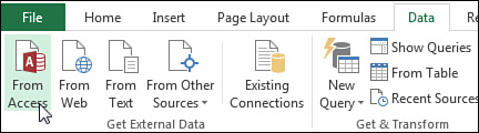
Excel 2016 offers a surprisingly easy way to use your Access data without creating two copies of it. To see how easy it is, open Excel and start a new workbook. Then click the Data tab and look for the group called Get External Data. Then click the From Access selection, as shown in Figure 7.18.
Clicking the From Access button activates a dialog asking you to select the database you want to work with. Select your database.
Tip
The sample database used in this chapter is available for download from www.mrexcel.com/pivotbookdata2016.html.
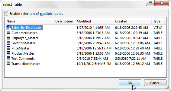
After your database has been selected, the dialog shown in Figure 7.19 appears. This dialog lists all the tables and queries available. In this example, select the query called Sales_By_Employee and click the OK button.
Note
In Figure 7.19, notice that the Select Table dialog contains a column called Type. There are two types of Access objects you can work with: views and tables. View indicates that the data set listed is an Access query, and Table indicates that the data set is an Access table.
In this example, notice that Sales_By_Employee is actually an Access query. This means that you import the results of the query. This is true interaction at work: Access does all the back-end data management and aggregation, and Excel handles the analysis and presentation!
Next, you see the Import Data dialog, where you select the format in which you want to import the data. As you can see in Figure 7.20, you have the option of importing the data as a table, as a pivot table, or as a pivot table with an accompanying pivot chart. You also have the option to tell Excel where to place the data.
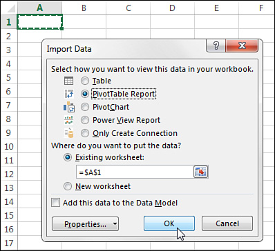
Select the radio button next to PivotTable Report, and click the OK button.
At this point, you should see the PivotTable Fields list shown in Figure 7.21. From here, you can use this pivot table just as you normally would.
The wonderful thing about this technique is that you can refresh the data simply by refreshing the pivot table. When you refresh, Excel takes a new snapshot of the data source and updates the pivot cache.
Caution
If you create a pivot table that uses an Access database as its source, you can refresh that pivot table only if the table or view is available. That is to say, deleting, moving, or renaming the database used to create the pivot table destroys the link to the external data set, thus destroying your ability to refresh the data. Deleting or renaming the source table or query has the same effect.
Following that reasoning, any clients using your linked pivot table cannot refresh the pivot table unless the source is available to them. If you need your clients to be able to refresh, you might want to make the data source available via a shared network directory.
Building a Pivot Table with SQL Server Data
In the spirit of collaboration, Excel 2016 vastly improves your ability to connect to transactional databases such as SQL Server. With the connection functionality found in Excel, creating a pivot table from SQL Server data is as easy as ever.
Start on the Data tab and select From Other Sources to see the drop-down menu shown in Figure 7.22. Then select From SQL Server.

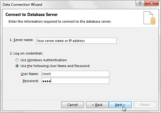
Selecting this option activates the Data Connection Wizard, as shown in Figure 7.23. The idea here is to configure your connection settings so Excel can establish a link to the server.
Note
There is no sample file for this example. The essence of this demonstration is the interaction between Excel and a SQL server data source. The actions you take to connect to your particular database are the same as demonstrated here.
You need to provide Excel with some authentication information. As you can see in Figure 7.23, you enter the name of your server as well as your username and password.
Note
If you are typically authenticated via Windows Authentication, you simply select the Use Windows Authentication option.
Next, you select the database with which you are working from a drop-down menu containing all available databases on the specified server. As you can see in Figure 7.24, a database called AdventureWorks2012 has been selected in the drop-down box. Selecting this database causes all the tables and views in it to be exposed in the list of objects below the drop-down menu. All that is left to do in this dialog is to choose the table or view you want to analyze and then click the Next button.

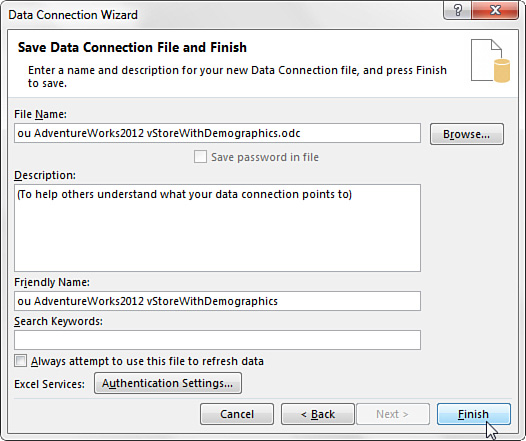
The next screen in the wizard, shown in Figure 7.25, enables you to enter some descriptive information about the connection you’ve just created.
Note
All the fields in the dialog shown in Figure 7.25 are optional edits only. That is, if you bypass this screen without editing anything, your connection works fine.
Here are the fields you’ll use most often:
![]() File Name—In the File Name input box, you can change the filename of the .odc (Office Data Connection) file generated to store the configuration information for the link you just created.
File Name—In the File Name input box, you can change the filename of the .odc (Office Data Connection) file generated to store the configuration information for the link you just created.
![]() Save Password in File—Under the File Name input box, you have the option of saving the password for your external data in the file itself (via the Save Password in File check box). Placing a check in this check box actually enters your password in the file. Keep in mind that this password is not encrypted, so anyone interested enough could potentially get the password for your data source simply by viewing your file with a text editor.
Save Password in File—Under the File Name input box, you have the option of saving the password for your external data in the file itself (via the Save Password in File check box). Placing a check in this check box actually enters your password in the file. Keep in mind that this password is not encrypted, so anyone interested enough could potentially get the password for your data source simply by viewing your file with a text editor.
![]() Description—In the Description field, you can enter a plain description of what this particular data connection does.
Description—In the Description field, you can enter a plain description of what this particular data connection does.
![]() Friendly Name—The Friendly Name field enables you to specify your own name for the external source. You typically enter a name that is descriptive and easy to read.
Friendly Name—The Friendly Name field enables you to specify your own name for the external source. You typically enter a name that is descriptive and easy to read.
When you are satisfied with your descriptive edits, click the Finish button to finalize your connection settings. You immediately see the Import Data dialog, shown in Figure 7.26. In it you select a pivot table and then click the OK button to start building your pivot table.

Leveraging Power Query to Extract and Transform Data
Every day, millions of Excel users manually pull data from some source location, manipulate that data, and integrate it into their pivot table reporting.
This process of extracting, manipulating, and integrating data is called ETL. ETL refers to the three separate functions typically required to integrate disparate data sources: extraction, transformation, and loading. The extraction function involves reading data from a specified source and extracting a desired subset of data. The transformation function involves cleaning, shaping, and aggregating data to convert it to the desired structure. The loading function involves actually importing or using the resulting data.
In an attempt to empower Excel analysts to develop robust and reusable ETL processes, Microsoft created Power Query. Power Query enhances the ETL experience by offering an intuitive mechanism to extract data from a wide variety of sources, perform complex transformations on that data, and then load the data into a workbook or the internal Data Model.
In the following sections, you’ll see how Power Query works and discover some of the innovative ways you can use it to help save time and automate the steps for importing clean data into your pivot table reporting models.
Power Query Basics
Although Power Query is relatively intuitive, it’s worth taking to the time to walk through a basic scenario to understand its high-level features. To start this basic look at Power Query, you need to import Microsoft Corporation stock prices from the past 30 days by using Yahoo Finance. For this scenario, you need to perform a web query to pull the data needed from Yahoo Finance. As shown in the following example, the Get & Transform group of the Data tab contains all the commands you need to start this query.
To start your query, follow these steps:
1. Select the New Query command on the Data tab and then select From Other Sources, From Web, as shown in Figure 7.27.

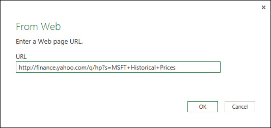
2. In the dialog box that appears (see Figure 7.28), enter in the URL for the data you need—in this case, http://finance.yahoo.com/q/hp?s=MSFT.
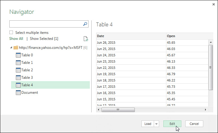
3. After a bit of gyrating, the Navigator pane shown in Figure 7.29 appears. Here, you select the data source you want extracted. You can click on each table to see a preview of the data. In this case, Table 4 holds the historical stock data you need, so click on Table 4 and then click the Edit button.
Note
You may have noticed that the Navigator pane shown in Figure 7.29 offers a Load button (next to the Edit button). The Load button allows you to skip any editing and import your targeted data as-is. If you are sure you will not need to transform or shape your data in any way, you can opt to click the Load button to import the data directly into the Data Model or a spreadsheet in your workbook.
Excel has another From Web command button on the Data tab under the Get External Data group. This unfortunate duplicate command is actually the legacy web scraping capability found in all Excel versions going back to Excel 2000.
The Power Query version of the From Web command (found under New Query, From Other Sources, From Web) goes beyond simple web scraping. Power Query is able to pull data from advanced web pages and is able to manipulate the data. Make sure you are using the correct feature when pulling data from the Web.
When you click the Edit button, Power Query activates a new Query Editor window, which contains its own Ribbon and a preview pane that shows a preview of the data (see Figure 7.30). Here, you can apply certain actions to shape, clean, and transform the data before importing.

The idea is to work with each column shown in the Query Editor, applying the necessary actions that will give you the data and structure you need. You’ll dive deeper into column actions later in this chapter. For now, you need to continue toward the goal of getting the last 30 days of stock prices for Microsoft Corporation.
4. Right-click the Date field to see the available column actions, as shown in Figure 7.31. Select Change Type and then Date to ensure that the Date field is formatted as a proper date.

5. Remove all the columns you do not need by right-clicking each one and clicking Remove. (Besides the Date field, the only other columns you need are the High, Low, and Close fields.) Alternatively, you can hold down the Ctrl key on your keyboard, select the columns you want to keep, right-click any of the selected columns, and then choose Remove Other Columns (see Figure 7.32).

Figure 7.32 Select the columns you do not want to keep and then select Remove Other Columns to get rid of them.
6. Ensure that the High, Low, and Close fields are formatted as proper numbers. To do this, hold down the Ctrl key on your keyboard, select the three columns, right-click, and then select Change Type, Decimal Number. After you do this, you may notice that some of the rows show the word Error. These are rows that contained text values that could not be converted.
7. Remove the Error rows by selecting Remove Errors from the Table Actions list (next to the Date field), as shown in Figure 7.33.
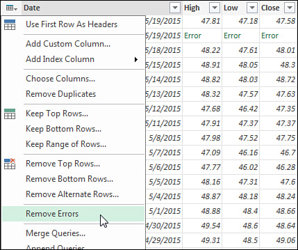
Figure 7.33 You can click the Table Actions icon to select actions (such as Remove Errors) that you want applied to the entire data table.
8. Once all the errors are removed, add a Week Of field that displays the week each date in the table belongs to. To do this, right-click the Date field and select the Duplicate Column option. A new column is added to the preview. Right-click the newly added column, select the Rename option, and then rename the column Week Of.
9. Select the Transform tab on the Power Query ribbon and then choose Date, Week, Start of the Week, as shown in Figure 7.34. Excel transforms the date to display the start of the week for a given date.
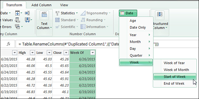
Figure 7.34 The Power Query ribbon can be used to apply transformation actions such as displaying the start of the week for a given date.
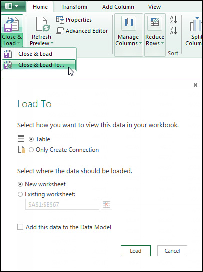
10. When you’ve finished configuring your Power Query feed, save and output the results. To do this, click the Close & Load drop-down found on the Home tab of the Power Query ribbon to reveal the two options shown in Figure 7.35. The Close & Load option saves your query and outputs the results to a new worksheet in your workbook as an Excel table. The Close & Load To option activates the Load To dialog box, where you can choose to output the results to a specific worksheet or to the internal Data Model. Alternatively, you can choose to save the query as a query connection only, which means you will be able to use the query in various in-memory processes without needing to actually output the results anywhere. Choose to output your results as a table on a new worksheet.
At this point, you will have a table similar to the one shown in Figure 7.36, which can be used to produce the pivot table you need.

Figure 7.36 Your final query pulled from the Internet—transformed, put into an Excel table, and ready to use in a pivot table.
Take a moment to appreciate what Power Query allowed you to do just now. With a few clicks, you searched the Internet, found some base data, shaped the data to keep only the columns you needed, and even manipulated that data to add an extra Week Of dimension to the base data. This is what Power Query is about: enabling you to easily extract, filter, and reshape data without the need for any programmatic coding skills.
Understanding Query Steps
Power Query uses its own formula language (known as the “M” language) to codify your queries. As with macro recording, each action you take when working with Power Query results in a line of code being written into a query step. Query steps are embedded M code that allow your actions to be repeated each time you refresh your Power Query data.
You can see the query steps for your queries by activating the Query Settings pane. Simply click the Query Settings command on the View tab of the Query Editor ribbon. You can also place a check in the Formula Bar option to enhance your analysis of each step with a formula bar that displays the syntax for the given step.
The Query Settings pane appears to the right of the preview pane, as shown in Figure 7.37. The formula bar is located directly above the preview pane.

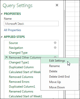
Figure 7.37 Query steps can be viewed and managed in the Applied Steps section of the Query Settings pane.
Each query step represents an action you took to get to a data table. You can click on any step to see the underlying M code in the Power Query formula bar. For example, clicking the step called Removed Errors reveals the code for that step in the formula bar.
Note
When you click on a query step, the data shown in the preview pane is a preview of what the data looked like up to and including the step you clicked. For example, in Figure 7.37, clicking the step before the Removed Other Columns step lets you see what the data looked like before you removed the non essential columns.
You can right-click on any step to see a menu of options for managing your query steps. Figure 7.38 illustrates the following options:
![]() Edit Settings—Edit the arguments or parameters that defines the selected step.
Edit Settings—Edit the arguments or parameters that defines the selected step.
![]() Rename—Give the selected step a meaningful name.
Rename—Give the selected step a meaningful name.
![]() Delete—Remove the selected step. Be aware that removing a step can cause errors if subsequent steps depend on the deleted step.
Delete—Remove the selected step. Be aware that removing a step can cause errors if subsequent steps depend on the deleted step.
![]() Delete Until End—Remove the selected step and all following steps.
Delete Until End—Remove the selected step and all following steps.
![]() Move Up—Move the selected step up in the order of steps.
Move Up—Move the selected step up in the order of steps.
![]() Move Down—Move the selected step down in the order of steps.
Move Down—Move the selected step down in the order of steps.
Refreshing Power Query Data
It’s important to note that Power Query data is not in any way connected to the source data used to extract it. A Power Query data table is merely a snapshot. In other words, as the source data changes, Power Query will not automatically keep up with the changes; you need to intentionally refresh your query.
If you chose to load your Power Query results to an Excel table in the existing workbook, you can manually refresh by right-clicking on the table and selecting the Refresh option.
If you chose to load your Power Query data to the internal Data Model, you need to open the Power Pivot window, select your Power Query data, and then click the Refresh command on the Home tab of the Power Query window.
To get a bit more automated with the refreshing of your queries, you can configure your data sources to automatically refresh your Power Query data. To do so, follow these steps:
1. Go to the Data tab in the Excel ribbon and select the Connections command. The Workbook Connections dialog box appears.
2. Select the Power Query data connection you want to refresh, and then click the Properties button.
3. With the Properties dialog box open, select the Usage tab.
4. Set the options to refresh the chosen data connection:
![]() Refresh Every X Minutes—Placing a check next to this option tells Excel to automatically refresh the chosen data every a specified number of minutes. Excel will refresh all tables associated with that connection.
Refresh Every X Minutes—Placing a check next to this option tells Excel to automatically refresh the chosen data every a specified number of minutes. Excel will refresh all tables associated with that connection.
![]() Refresh Data When Opening the File—Placing a check next to this option tells Excel to automatically refresh the chosen data connection upon opening the workbook. Excel will refresh all tables associated with that connection as soon as the workbook is opened.
Refresh Data When Opening the File—Placing a check next to this option tells Excel to automatically refresh the chosen data connection upon opening the workbook. Excel will refresh all tables associated with that connection as soon as the workbook is opened.
These refresh options are useful when you want to ensure that your customers are working with the latest data. Of course, setting these options does not preclude the ability manually refresh the data using the Refresh command on the Home tab.
Managing Existing Queries
As you add various queries to a workbook, you will need a way to manage them. Excel accommodates this need by offering the Workbook Queries pane, which enables you to edit, duplicate, refresh, and generally manage all the existing queries in the workbook. Activate the Workbook Queries pane by selecting the Show Queries command on the Data tab of the Excel ribbon.
You need to find the query you want to work with and then right-click it to take any one of these actions (see Figure 7.39):
![]() Edit—Open the Query Editor, where you can modify the query steps.
Edit—Open the Query Editor, where you can modify the query steps.
![]() Delete—Delete the selected query.
Delete—Delete the selected query.
![]() Refresh—Refresh the data in the selected query.
Refresh—Refresh the data in the selected query.
![]() Load To—Activate the Load To dialog box, where you can redefine where the selected query’s results are used.
Load To—Activate the Load To dialog box, where you can redefine where the selected query’s results are used.
![]() Duplicate—Create a copy of the query.
Duplicate—Create a copy of the query.
![]() Reference—Create a new query that references the output of the original query.
Reference—Create a new query that references the output of the original query.
![]() Merge—Merge the selected query with another query in the workbook by matching specified columns.
Merge—Merge the selected query with another query in the workbook by matching specified columns.
![]() Append—Append the results of another query in the workbook to the selected query.
Append—Append the results of another query in the workbook to the selected query.
![]() Send to Data Catalog—Publish and share the selected query via a Power BI server that your IT department sets up and manages.
Send to Data Catalog—Publish and share the selected query via a Power BI server that your IT department sets up and manages.
![]() Move to Group—Move the selected query into a logical group you create for better organization.
Move to Group—Move the selected query into a logical group you create for better organization.
![]() Move Up—Move the selected query up in the Workbook Queries pane.
Move Up—Move the selected query up in the Workbook Queries pane.
![]() Move Down—Move the selected query down in the Workbook Queries pane.
Move Down—Move the selected query down in the Workbook Queries pane.
![]() Show the Peek—Show a preview of the query results for the selected query.
Show the Peek—Show a preview of the query results for the selected query.
![]() Properties—Rename the query and add a friendly description.
Properties—Rename the query and add a friendly description.
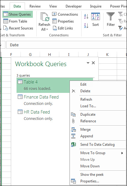
Figure 7.39 Right-click any query in the Workbook Queries pane to see the available management options.
The Workbook Queries pane is especially useful when your workbook contains several queries. Think of it as a kind of table of contents that allows you to easily find and interact with the queries in your workbook.
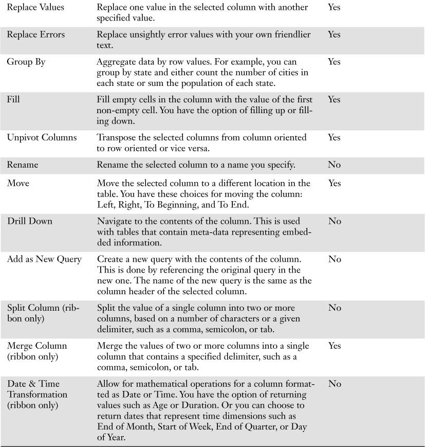
Understanding Column-Level Actions
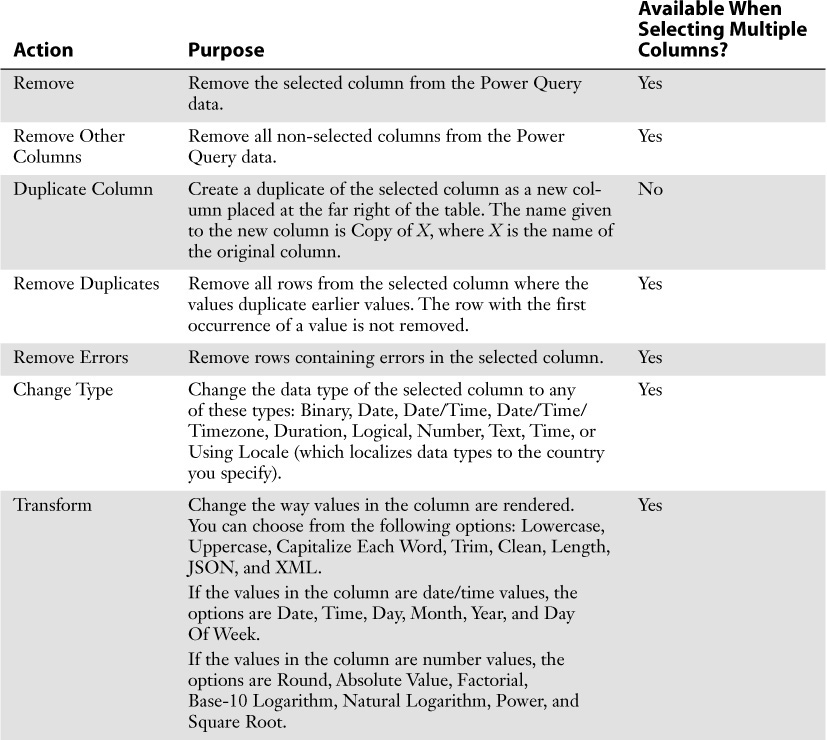
Right-clicking a column in the Query Editor activates a context menu that shows a full list of the actions you can take. You can also apply certain actions to multiple columns at one time by selecting two or more columns before right-clicking. Figure 7.40 shows the available column-level actions, and Table 7.2 explains them, as well as a few other actions that are available only in the Query Editor ribbon.
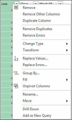
Figure 7.40 Right-click any column to see the column-level actions you can use to transform the data.
Note
Note that all of the column-level actions available in Power Query are also available in the Query Editor ribbon. So you can either opt for the convenience of right-clicking to quickly select an action or choose to utilize the more visual ribbon menu. There are a few useful column-level actions found only in the ribbon (see Table 7.2).
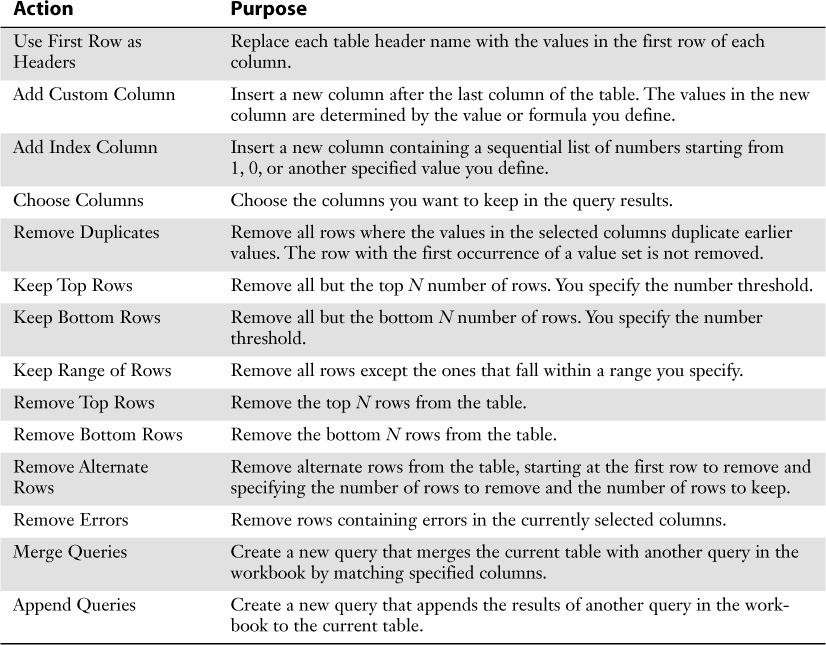
Understanding Table Actions
While you’re in the Query Editor, Power Query allows you to apply certain actions to an entire data table. You can see the available table-level actions by clicking the Table Actions icon shown in Figure 7.41.
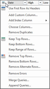
Figure 7.41 Click the Table Actions icon in the upper-left corner of the Query Editor Preview pane to see the table-level actions you can use to transform the data.
Table 7.3 lists the table-level actions and describes the primary purpose of each one.
Note
Note that all of the table-level actions available in Power Query are also available in the Query Editor ribbon. So you can either opt for the convenience of right-clicking to quickly select an action or choose to utilize the more visual ribbon menu.
Power Query Connection Types
Microsoft has invested a great deal of time and resources in ensuring that Power Query has the ability to connect to a wide array of data sources. Whether you need to pull data from an external website, a text file, a database system, Facebook, or a web service, Power Query can accommodate most, if not all, your source data needs.
You can see all the available connection types by clicking on the New Query drop-down on the Data tab. As Figure 7.42 shows, Power Query offers the ability to pull from a wide array of data sources:
![]() From File—Pull data from a specified Excel file, text file, CSV file, XML file, or folder.
From File—Pull data from a specified Excel file, text file, CSV file, XML file, or folder.
![]() From Database—Pull data from a relational Microsoft Access, SQL Server, or SQL Server Analysis Services database.
From Database—Pull data from a relational Microsoft Access, SQL Server, or SQL Server Analysis Services database.
![]() From Other Sources—Pull data from a wide array of Internet, cloud, and other ODBC data sources.
From Other Sources—Pull data from a wide array of Internet, cloud, and other ODBC data sources.
![]() From Table—Query data from a defined Excel Table within the current workbook.
From Table—Query data from a defined Excel Table within the current workbook.

Figure 7.42 Power Query has the ability to connect to a wide array of text, database, and Internet data sources.
Clicking any of the connection types shown in Figure 7.42 activates a set of dialog boxes for the selected connection. These dialog boxes ask for the basic parameters Power Query needs to connect to the data source—parameters such as file path, URL, server name, and credentials.
Each connection type requires its own unique set of parameters, so each of their dialog boxes are different. Luckily, Power Query rarely needs more than a handful of parameters to connect to any one data source, so the dialog boxes are relatively intuitive and hassle free.
Power Query saves the data source parameters for each data source connection you have used. You can view, edit, or delete any of the data source connections by selecting Data Source Settings at the bottom of the New Query drop-down (see Figure 7.43). Click any of the connections in the Data Source Settings pane to edit or delete the selected connection.
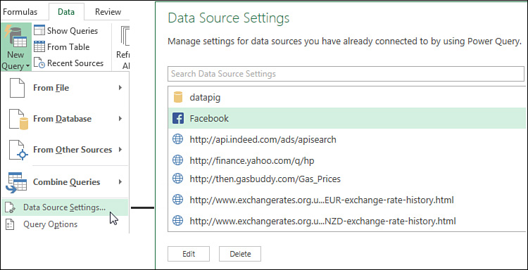
Figure 7.43 The Data Source Settings pane allows you to edit and delete previously used data connections.
Caution
Deleting a connection does not delete any of its associated data that you may have already loaded in your workbook or internal Data Model. However, when you try to refresh the data, Power Query won’t have any of the connection parameters (because you deleted them), so it will ask you for the connection parameters again.
Case Study: Transposing a Data Set with Power Query
In Chapter 2, “Creating a Basic Pivot Table,” you learned that the perfect layout for the source data in a pivot table is Tabular layout. Tabular layout is a particular table structure where there are no blank rows or columns, every column has a heading, every field has a value in every row, and columns do not contain repeating groups of data.
Unfortunately, you often encounter data sets like the one shown in Figure 7.44. The problem here is that the month headings are spread across the top of the table, doing double duty as column labels and actual data values. In a pivot table, this format would force you to manage and maintain 12 fields, each representing a different month.
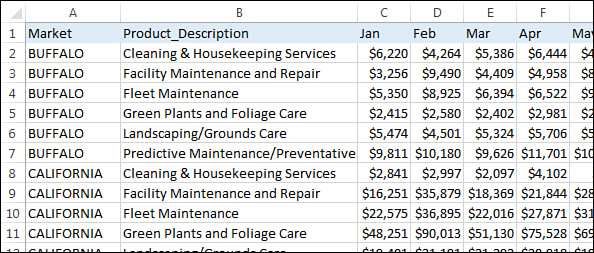
Figure 7.44 You need to convert this matrix-style table to a Tabular data set so it can be used in a pivot table.
You can leverage Power Query to easily transform this matrix-style data set to one that is appropriate for use with a pivot table. Follow these steps:
1. Place your cursor inside your data table and select Insert, Table. In the resulting Create Table dialog box, specify the range for your data. Excel turns that range into a defined table that Power Query can recognize.
2. On the Data tab, select From Table to use your newly created table as the source for the query. The Query Editor appears.
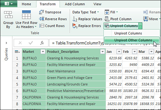
3. In the Query Editor, hold down the Ctrl key as you select the Market and Product_Description fields (which are the fields you do not want to transpose).
4. Go to the Transform tab on the Query Editor ribbon, select the Unpivot Columns drop-down, and then select Unpivot Other Columns (see Figure 7.45). All of the month names now fall under a column called Attributes.
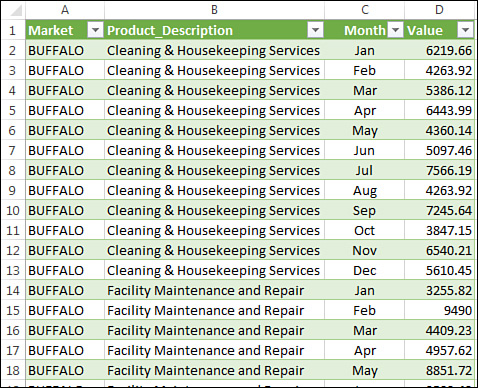
5. Rename the Attributes column Month.
6. Click the Home tab on the Query Editor ribbon and select the Close & Load command to send the results to a new worksheet in the current workbook.
Amazingly, that is it! If all went well, you should now have a table similar to the one shown in Figure 7.46.
In just a few clicks, you were able to transpose your data set in preparation for use in a pivot table. Even better, this query can be refreshed! So as new month columns or rows are added to the source table, Power Query will rerun your steps and automatically include any new data in the resulting table.
The new Power Query functionality is an exciting addition to Excel 2016. In the past, it was a chore to import and clean external data in preparation for pivot table reporting. Now with Power Query, you can create automated extraction and transformation procedures that traditionally would require personnel and skillsets found only in the IT department.
Next Steps
Chapter 8, “Sharing Pivot Tables with Others,” covers the ins and outs of sharing pivot tables with the world. In that chapter, you will find out how you can distribute your pivot tables through the Web.