11 Building More Powerful Worksheets
Introduction
Excel also includes a variety of add-ins—programs that provide added functionality—to increase your efficiency. Some of these supplemental programs—including Analysis ToolPak, Analysis ToolPak VBA, Euro Currency, and Solver—are useful to almost anyone using Excel. Others, such as the Analysis ToolPak, add customized features, functions, or commands specific to use in financial, statistical, and other highly specialized fields. The purpose of each of these customization features is the same—to make Excel even easier to use and to enable you to accomplish more with less effort.
Before you can use an Excel or a third-party add-in, you need to load it first. When you load an add-in, the feature may also add a command to a Ribbon tab or toolbar. You can load one or more add-ins. If you no longer need an add-in, you should unload it to save memory and reduce the number of commands on a Ribbon tab. When you unload an add-in, you may also need to restart Excel to remove an add-in command from a Ribbon tab.
If your worksheet or workbook needs to go beyond simple calculations, Microsoft Excel offers several tools to help you create more specialized projects. With Excel, you can perform “what if” analysis using several different methods to get the results you want.
Using Data Analysis Tools
Excel provides a collection of statistical functions and macros to analyze data in the Analysis ToolPak. The Analysis Toolpak is an add-in program, which may need to be loaded using the Add-In pane in Excel Options. The tools can be used for a variety of scientific and engineering purposes and for general statistical analysis. You provide the data, and the tools use the appropriate functions to determine the result. To effectively use these tools, you need to be familiar with the area of statistics or engineering for which you want to develop an analysis. You can view a list of all the tools in the Data Analysis dialog box. For additional information about each tool, see the online Help.
Use Data Analysis Tools
![]() Click the Data tab.
Click the Data tab.
![]() Click the Data Analysis button. If not available, load the add-in.
Click the Data Analysis button. If not available, load the add-in.
![]() Click the analysis tool you want to use.
Click the analysis tool you want to use.
![]() To get help about each tool, click Help.
To get help about each tool, click Help.
![]() Click OK.
Click OK.
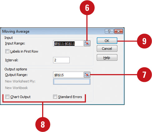
![]() Select or enter the input range (a single row or column). You can use the Collapse Dialog button to select a range and the Expand Dialog button to return.
Select or enter the input range (a single row or column). You can use the Collapse Dialog button to select a range and the Expand Dialog button to return.
![]() Select or enter the output range. You can use the Collapse Dialog button to select a range and the Expand Dialog button to return.
Select or enter the output range. You can use the Collapse Dialog button to select a range and the Expand Dialog button to return.
![]() Specify any additional tool-specific options you want.
Specify any additional tool-specific options you want.
![]() Click OK.
Click OK.

Using the Euro Conversion
The Euro Conversion Wizard helps you convert data from one european currency to another. Excel provides this feature as an add-in program, which may need to be loaded using the Add-In pane in Excel Options. The wizard guides you through the process to convert specified data from one european currency to another. All you need to do is specify the source and destination range, currency conversion from and to, and an output format.
Use the Euro Conversion
![]() Click the Formulas tab.
Click the Formulas tab.
![]() Select the data you want to convert.
Select the data you want to convert.
![]() Click the Euro Conversion button.
Click the Euro Conversion button.
![]() Specify a source and destination range for the conversion.
Specify a source and destination range for the conversion.
You can use the Collapse Dialog button to select a range and the Expand Dialog button to return.
![]() Click the From list arrow, select a From currency, click the To list arrow, and then select a To currency.
Click the From list arrow, select a From currency, click the To list arrow, and then select a To currency.
![]() Click the Output format list arrow, and then select an output format.
Click the Output format list arrow, and then select an output format.
![]() Click OK.
Click OK.

Looking at Alternatives with Data Tables
Data tables provide a shortcut by calculating all of the values in one operation. A data table is a range of cells that shows the results of substituting different values in one or more formulas. For example, you can compare loan payments for different interest rates. There are two types of data tables: one-input and two-input. With a one-input table, you enter different values for one variable and see the effect on one or more formulas. With a two-input table, you enter values for two variables and see the effect on one formula.
Create a One-Input Data Table
![]() Enter the formula you want to use.
Enter the formula you want to use.
If the input values are listed down a column, specify the new formula in a blank cell to the right of an existing formula in the top row of the table. If the input values are listed across a row, enter the new formula in a blank cell below an existing formula in the first column of the table.
![]() Select the data table, including the column or row that contains the new formula.
Select the data table, including the column or row that contains the new formula.
![]() Click the Data tab.
Click the Data tab.
![]() Click the What-If Analysis button, and then click Data Table.
Click the What-If Analysis button, and then click Data Table.
![]() Enter the input cell.
Enter the input cell.
If the input values are in a column, enter the reference for the input cell in the Column Input Cell box. If the input values are in a row, enter the reference for the input cell in the Row Input Cell box.
![]() Click OK.
Click OK.

Asking “What If” with Goal Seek
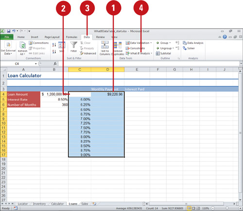
Excel functions make it easy to create powerful formulas, such as calculating payments over time. Sometimes, however, being able to make these calculations is only half the battle. Your formula might tell you that a monthly payment amount is $2,000, while you might only be able to manage a $1,750 payment. Goal Seek enables you to work backwards to a desired result, or goal, by adjusting the input values.
Create a “What-If” Scenario with Goal Seek
![]() Click any cell within the list range.
Click any cell within the list range.
![]() Click the Data tab.
Click the Data tab.
![]() Click the What-If Analysis button, and then click Goal Seek.
Click the What-If Analysis button, and then click Goal Seek.
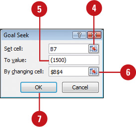
![]() Click the Set Cell box, and then type the cell address you want to change.
Click the Set Cell box, and then type the cell address you want to change.
You can also click the Collapse Dialog button, use your mouse to select the cells, and then click the Expand Dialog button.
![]() Click the To Value box, and then type the result value.
Click the To Value box, and then type the result value.
![]() Click the By Changing Cell box, and then type the cell address you want Excel to change.
Click the By Changing Cell box, and then type the cell address you want Excel to change.
You can also click the Collapse Dialog button, use your mouse to select the cells, and then click the Expand Dialog button.
![]() Click OK.
Click OK.
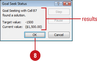
The Goal Seek Status dialog box, opens displaying the goal seek results.
![]() Click OK.
Click OK.

Creating Scenarios
Because some worksheet data is constantly evolving, the ability to create multiple scenarios lets you speculate on a variety of outcomes. For example, the marketing department might want to see how its budget would be affected if sales decreased by 25 percent. Although it’s easy enough to plug in different numbers in formulas, Excel allows you to save these values and then recall them at a later time.
Create and Show a Scenario
![]() Click the Data tab.
Click the Data tab.
![]() Click the What-If Analysis button, and then click Scenario Manager.
Click the What-If Analysis button, and then click Scenario Manager.
![]() Click Add.
Click Add.
![]() Type a name that identifies the scenario.
Type a name that identifies the scenario.
![]() Type the cells you want to modify in the scenario, or click the Collapse Dialog button, use your mouse to select the cells, and then click the Expand Dialog button.
Type the cells you want to modify in the scenario, or click the Collapse Dialog button, use your mouse to select the cells, and then click the Expand Dialog button.
![]() If you want, type a comment.
If you want, type a comment.
![]() If you want, select the Prevent changes check box to protect the cell.
If you want, select the Prevent changes check box to protect the cell.
![]() Click OK.
Click OK.
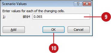
![]() Type values for each of the displayed changing cells.
Type values for each of the displayed changing cells.
![]() Click OK.
Click OK.
![]() Click Close.
Click Close.


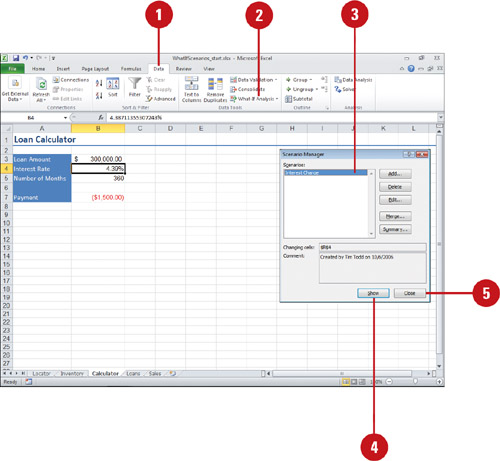
Show a Scenario
![]() Click the Data tab.
Click the Data tab.
![]() Click the What-If Analysis button, and then click Scenario Manager.
Click the What-If Analysis button, and then click Scenario Manager.
![]() Select the scenario you want to see.
Select the scenario you want to see.
![]() Click Show.
Click Show.
![]() Click Close.
Click Close.
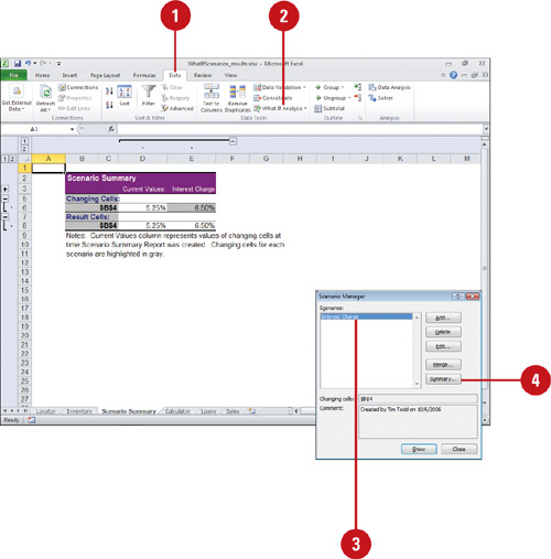
Create a Scenario Summary or PivotTable Report
![]() Click the Data tab.
Click the Data tab.
![]() Click the What-If Analysis button, and then click Scenario Manager.
Click the What-If Analysis button, and then click Scenario Manager.
![]() Select the scenario you want to see.
Select the scenario you want to see.
![]() Click Summary.
Click Summary.
![]() Click the Scenario summary or Scenario PivotTable report option.
Click the Scenario summary or Scenario PivotTable report option.
![]() Click OK.
Click OK.
A scenario summary worksheet tab appears with the report.
Using Solver
The Solver (New!) is similar to Goal Seek and scenarios, but provides more options to restrict the allowable range of values for different cells that can affect the goal. The Solver is an add-in program, which may need to be loaded using the Add-In pane in Excel Options. The Solver is useful for predicting how results might change over time based on different assumptions. For example, suppose you have sales goals and quotas for the next three months. The Solver can take the expectations and the current quotas for each month, and determine how sales quotas for all three amounts be adjusted to achieve the goal.
Use Solver
![]() Click the Data tab.
Click the Data tab.
![]() Click the Solver button.
Click the Solver button.
![]() Select the target cell.
Select the target cell.
![]() Click an Equal To option, and then, if necessary, enter a value.
Click an Equal To option, and then, if necessary, enter a value.
![]() Select the range of cells the solver uses to compare against the target cell.
Select the range of cells the solver uses to compare against the target cell.
![]() Click Add.
Click Add.
![]() Enter specific cell reference and constraint, and then click Add. You can specify several cell constraints.
Enter specific cell reference and constraint, and then click Add. You can specify several cell constraints.
![]() Click OK.
Click OK.
![]() To modify the constraints, click any of the following:
To modify the constraints, click any of the following:
![]() Change. Select a constraint, and then click Change to modify it.
Change. Select a constraint, and then click Change to modify it.
![]() Delete. Select a constraint, and then click Delete to remove it.
Delete. Select a constraint, and then click Delete to remove it.
![]() Reset All. Click Reset All to rest all Solver options and cell selection.
Reset All. Click Reset All to rest all Solver options and cell selection.
![]() Load/Save. Click Load/Save to select a range holding a saved model (to load) or select an empty range with a specified number of cells (to save).
Load/Save. Click Load/Save to select a range holding a saved model (to load) or select an empty range with a specified number of cells (to save).

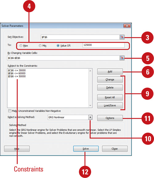
![]() Click the Solving Method list arrow, and then select a method:
Click the Solving Method list arrow, and then select a method:
![]() GRG Nonlinear. Select for smooth nonlinear problems.
GRG Nonlinear. Select for smooth nonlinear problems.
![]() Simplex LP. Select for linear problems.
Simplex LP. Select for linear problems.
![]() Evolutionary. Select for non-smooth problems.
Evolutionary. Select for non-smooth problems.
![]() To set options for each of the solving methods, click Options, click the tab you want (All Methods, GRG NonLinear, or Evolutionary), select the options you want, and then click OK.
To set options for each of the solving methods, click Options, click the tab you want (All Methods, GRG NonLinear, or Evolutionary), select the options you want, and then click OK.
![]() Click Solve.
Click Solve.
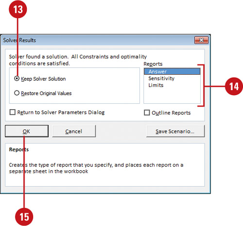
If the Solver finds a solution, the Solver Results dialog box opens.
![]() Click the Keep Solver Solution option.
Click the Keep Solver Solution option.
![]() Click a report type.
Click a report type.
![]() Click OK.
Click OK.

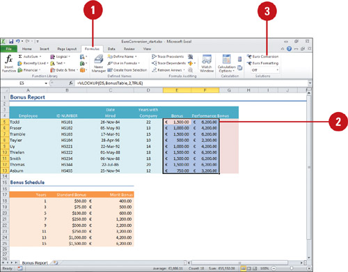
Using Lookup and Reference Functions
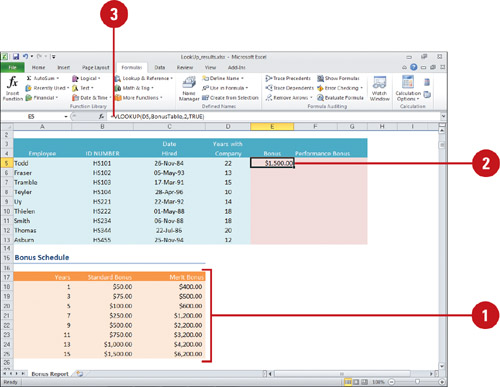
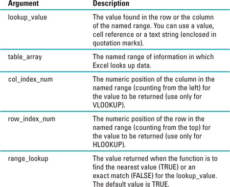
You can use lookup and reference functions in Excel to easily retrieve information from a data list. The lookup functions (VLOOKUP and HLOOKUP) allow you to search for and insert a value in a cell that is stored in another place in the worksheet. The HLOOKUP function looks in rows (a horizontal lookup) and the VLOOKUP function looks in columns (a vertical lookup). Each function uses four arguments (pieces of data) as shown in the following definition: =VLOOKUP (lookup_value, table_array, col_index_num, range_lookup). The VLOOKUP function finds a value in the left-most column of a named range and returns the value from the specified cell to the right of the cell with the found value, while the HLOOKUP function does the same to rows. In the example, =VLOOKUP(12,Salary,2,TRUE), the function looks for the value 12 in the named range Salary and finds the closest (next lower) value, and returns the value in column 2 of the same row and places the value in the active cell. In the example, =HLOOKUP (“Years”,Salary,4,FALSE), the function looks for the value “Years” in the named range Salary and finds the exact text string value, and then returns the value in row 4 of the column.
Use the VLOOKUP Function
![]() Create a data range in which the left-most column contains a unique value in each row.
Create a data range in which the left-most column contains a unique value in each row.
![]() Click the cell where you want to place the function.
Click the cell where you want to place the function.
![]() Type =VLOOKUP (value, named range, column, TRUE orFALSE), and then press Enter.
Type =VLOOKUP (value, named range, column, TRUE orFALSE), and then press Enter.
Or click the Formulas tab, click the Look & Reference button, click VLOOKUP, specify the function arguments, and then click OK.
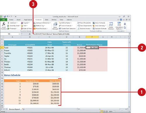
Use the HLOOKUP Function
![]() Create a data range in which the uppermost row contains a unique value in each row.
Create a data range in which the uppermost row contains a unique value in each row.
![]() Click the cell where you want to place the function.
Click the cell where you want to place the function.
![]() Type =HLOOKUP(value, named range, row, TRUE or FALSE), and then press Enter.
Type =HLOOKUP(value, named range, row, TRUE or FALSE), and then press Enter.
Or click the Formulas tab, click the Look & Reference button, click HLOOKUP, specify the function arguments, and then click OK.
Using Text Functions
You can use text functions to help you work with text in a workbook. If you need to count the number of characters in a cell or the number of occurrences of a specific text string in a cell, you can use the LEN and SUBSTITUTE functions. If you want to narrow the count to only upper or lower case text, you can use the UPPER and LOWER functions. If you need to capitalize a list of names or titles, you can use the PROPER function. The function capitalizes the first letter in a text string and converts all other letters to lowercase.
Use Text Functions
![]() Create a data range in which the left-most column contains a unique value in each row.
Create a data range in which the left-most column contains a unique value in each row.
![]() Click the cell where you want to place the function.
Click the cell where you want to place the function.
![]() Type = (equal sign), type a text function, specify the argument for the selected function, and then press Enter.
Type = (equal sign), type a text function, specify the argument for the selected function, and then press Enter.
Some examples include:
![]()
=LEFT(A4,FIND(“ “,A4)-1)
![]()
=RIGHT(A4, LEN(A4-FIND(“*”, SUBSTITUTE(A4,” “,”*”, LEN(A4)-LEN(SUBSTITUTE(A4,” “,”“)))))
![]()
=UPPER(A4)
![]()
=LOWER(A4)
![]()
=PROPER(A4)
Or click the Formulas tab, click the Text button, click a function, specify the function arguments, and then click OK.

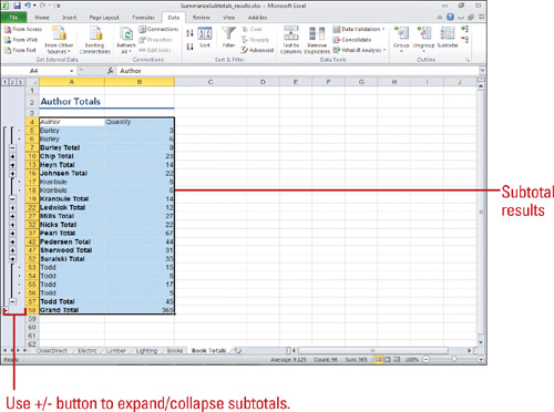
Summarizing Data Using Subtotals
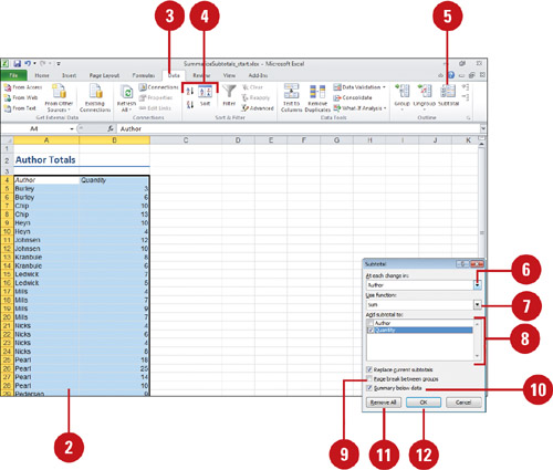
If you have a column list with similar facts and no blanks, you can automatically calculate subtotals and grand totals in a list. Subtotals are calculated with a summary function, such as SUM, COUNT, or AVERAGE, while Grand totals are created from detailed data instead of subtotal values. Detailed data is typically adjacent to and either above or below or to the left of the summary data. When you summarize data using subtotals, the data list is also outlined to display and hide the detailed rows for each subtotal.
Subtotal Data in a List
![]() Organize data in a hierarchical fashion—place summary rows below detail rows and summary columns to the right of detail columns.
Organize data in a hierarchical fashion—place summary rows below detail rows and summary columns to the right of detail columns.
![]() Select the data that you want to subtotal.
Select the data that you want to subtotal.
![]() Click the Data tab.
Click the Data tab.
![]() Use sort buttons to sort the column.
Use sort buttons to sort the column.
![]() Click the Subtotal button.
Click the Subtotal button.
![]() Click the column to subtotal.
Click the column to subtotal.
![]() Click the summary function you want to use to calculate the subtotals.
Click the summary function you want to use to calculate the subtotals.
![]() Select the check box for each column that contains values you want to subtotal.
Select the check box for each column that contains values you want to subtotal.
![]() To set automatic page breaks following each subtotal, select the Page break between groups check box.
To set automatic page breaks following each subtotal, select the Page break between groups check box.
![]() To show or hide a summary row above the detail row, select or clear the Summary below data check box.
To show or hide a summary row above the detail row, select or clear the Summary below data check box.
![]() To remove subtotals, click Remove All.
To remove subtotals, click Remove All.
![]() Click OK.
Click OK.
![]() To add more subtotals, use the Subtotal button again.
To add more subtotals, use the Subtotal button again.
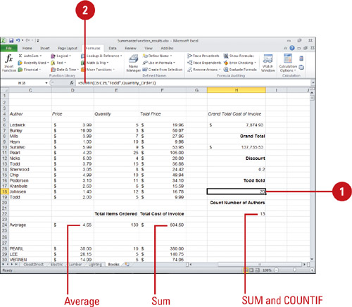
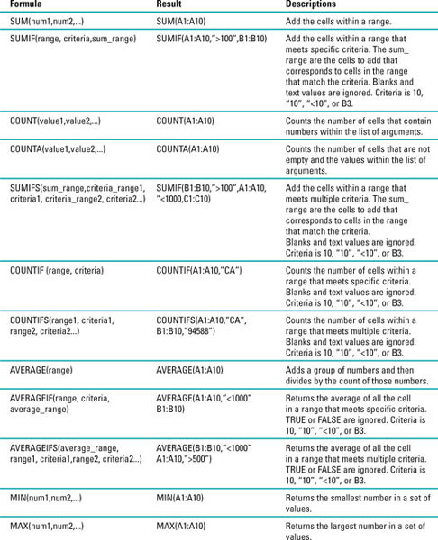
Summarizing Data Using Functions
You can use conditional functions, such as SUMIF, COUNTIF, and AVER-AGEIF to summarize data in a workbook. These functions allow you to calculate a total, count the number of items, and average a set of numbers based on a specific criteria. You can use the SUMIF function to add up interest payment for accounts over $100, or use the COUNTIF function to find the number of people who live in CA from an address list. If you need to perform these functions based on multiple criteria, you can use the SUMIFS, COUNTIFS, and AVERAGEIFS functions. If you need to find the minimum or maximum in a range, you can use the summarizing functions MIN and MAX.
Use Summarize Data Functions
![]() Click the cell where you want to place the function.
Click the cell where you want to place the function.
![]() Type = (equal sign), type a text function, specify the argument for the selected function, and then press Enter.
Type = (equal sign), type a text function, specify the argument for the selected function, and then press Enter.
Some examples include:
![]()
=AVERAGE(D6:D19)
![]()
={=SUM(1/COUNTIF(C6:C19, C6:19))}
![]()
=SUMIF(C6:C19,”Todd”, Quantity_Order1)
![]()
=SUM(Quantity_Order1)
Or click the Formulas tab, click the Math & Trig button or click the More Functions button and point to Statistical, click a data function, specify the function arguments, and then click OK.
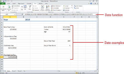
Using Date & Time Functions
Calculating Dates
You can use different formulas to return a specific date. Here are some common examples you can use.
Calculate a Specific Day
You can use the DATE function to quickly calculate a specific day, such as New Year’s (January 1st), US Independence Day (July 4th), or Christmas (December 25th).
=DATE(A1,1,1)
=DATE(A1,7,4)
=DATE(A1,12,25)
Calculate a Changing Day
You can use the DATE and WEEKDAY function to calculate a holiday that changes each year, such as Thanksgiving, which is celebrated on the fourth Thursday in November.
=DATE(A1,11,1)+IF(5<WEEKDAY (DATE(A1,11,1)),
7-WEEKDAY(DATE(A1,11,1))+5,
5-WEEKDAY(DATE(A1,11,1)))+((4-1)*7)
Calculate the Day of the Year
You can calculate the day of the year for a specific date in the A1 cell. This function returns an integer between 1 and 365.
=A1-DATE(YEAR(A1),1,0)
Calculate the Day of the Week
You can use the WEEKDAY function to calculate the day of the week for a specific date in a cell. The function returns an integer between 1 and 7. This example returns 1 for Sunday, October 7, 2010.
=WEEKDAY(DATE(2010, 10,7))
Calculate a Person’s Age
You can use the DATEIF function to calculate the age of a person. The function returns an integer. For this example, A1 is birth date, A2 is the current date, and “y” indicates years (“md” indicates days and “ym” indicates months). If you loaded the Analysis ToolPak, you can also use the INT function.
=DATEIF(A1, A2,”y”) or INT(YEARFRAC(A1, A2))
Excel stores dates as sequential serial numbers so that they can be used in calculations. By default, January 1, 1900 is serial number 1 and each day counts up from there.
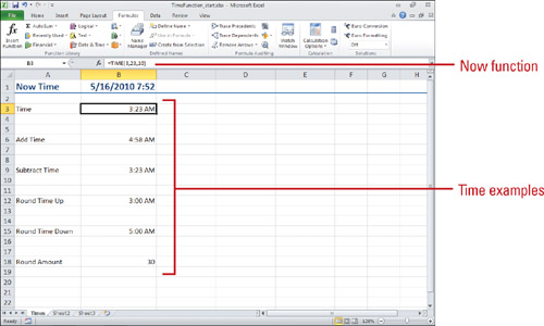
Working with Time
You can use different formulas to work with time. Here are some common examples you can use.
Display the Current Date and Time
You can use the NOW function to quickly display the current date and time. To display the current date and time, use the function:
=NOW()
Add Times
You can use the TIME function to quickly add different times together. To add 1 hour, 35 minutes, 10 seconds to a time in A1, use the function:
=A1 + TIME(1, 35, 10)
Subtract Times
You can use the TIME function to subtract one time from another. To subtract 1 hour, 35 minutes, 10 seconds from a time in A1, use the function:
=A1 - TIME(1, 35, 10)
Rounding Times
You can use the TIME function along with the HOUR and MINUTE functions to round time up or down to the nearest time interval. To round to the previous interval (always going earlier or staying the same), use the function:
=TIME(HOUR(A1), FLOOR(MINUTE(A1), B1,0)
To round to the next interval (always going later or staying the same), use the function:
=TIME(HOUR(A1), CEILING(MINUTE(A1), B1,0)
The FLOOR and CEILING functions are Math & Trig functions for rounding numbers.
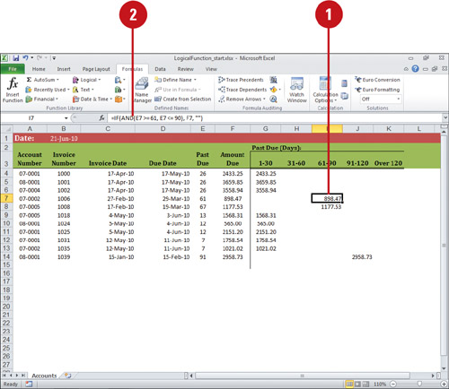
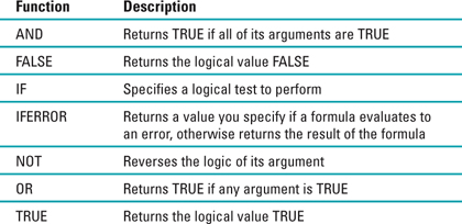
Using Logical Functions
You can use logical functions to help you test whether conditions are true or false or make comparisons between expressions. The logical functions in Excel include: AND, FALSE, IF, IFERROR, NOT, OR, and TRUE. The structure of the IF function is IF(logical_test, value_if_false, value_if_false). For example, IF(E6<31, F6,”“). If E6 is less than 31, then display the contents of F6; if not, then display nothing. You can also nest logical functions within a logical function. For example, IF(AND(E7>=61, E7<=90), F7,”“). If E7 is greater than or equal to 61 and less than or equal to 61, then display the contents of F7; if not, then display nothing.
Use Logical Functions
![]() Click the cell where you want to place the function.
Click the cell where you want to place the function.
![]() Type = (equal sign), type a text function, specify the argument for the selected function, and then press Enter.
Type = (equal sign), type a text function, specify the argument for the selected function, and then press Enter.
Some syntax examples include:
![]() =IF(logical_test, value_if_false, value_if_false)
=IF(logical_test, value_if_false, value_if_false)
Some examples include:
![]()
=IF(E6<31, F6,”“)
![]()
=IF(AND(E7>=61, E7<=90), F7,”“)
![]()
=IF(NOT(A2<=15),”Goal”,”Not Goal”)
Or click the Formulas tab, click the Logical button, click a function, specify the function arguments, and then click OK.
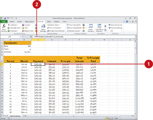
Using Financial Functions
You can use financial functions to help you work with formulas related to business, accounting, and investment. You can use formulas for depreciation, such as SLN (Straight-Line Depreciation) and SYD (Sum-of-Years’ Digits), or formulas for interest and investments, such as FV (Future Value of an investment), EFFECT (Effective annual interest rate) or IPMT (Interest Payment for an investment or loan). Many of the investment functions use the following arguments: rate, nominal_rate, per, nper, pv, fv, pmt, and type. Rate is the interest rate per period; Nominal_rate is the nominal interest rate; Per is the period for which you want to find the interest (between 1 and nper); Nper is the total number of payments periods; Pv is the present value; Fv is the future value; Pmt is the payment made each period; and Type is the number 0 or 1 to indicate when payments are due (0 at the end of the period or 1 at the beginning of the period). Many of the depreciation functions use the following arguments: cost, salvage, and life. Cost is the initial cost of the asset; Salvage is the value at the end of the depreciation; Life is the number of periods the asset is depreciated.
Use Financial Functions
![]() Click the cell where you want to place the function.
Click the cell where you want to place the function.
![]() Type = (equal sign), type a text function, specify the argument for the selected function, and then press Enter.
Type = (equal sign), type a text function, specify the argument for the selected function, and then press Enter.
Some syntax examples include:
![]() =FV(rate, nper, pmt, pv, type)
=FV(rate, nper, pmt, pv, type)
![]() =EFFECT(nominal_rate, npery)
=EFFECT(nominal_rate, npery)
![]() =IPMT(rate, per, nper, pv, fv, type)
=IPMT(rate, per, nper, pv, fv, type)
![]() =SLN(cost, salvage, life)
=SLN(cost, salvage, life)
![]() =SYD(cost, salvage, life, per)
=SYD(cost, salvage, life, per)
Or click the Formulas tab, click the Financial button, click a function, specify the function arguments, and then click OK.
Using Math Functions
You can use math & trigonometry functions to help you perform mathematical calculations. You can use formulas for calculations, such as SQRT (Square root) or TAN (Tangent); formulas for conversion, such as DEGREES (radians to Degrees), or RADIANS (degrees to Radians); or formulas for rounding, such as FLOOR (number down, toward zero), CEILING (number up, towards nearest integer), INT (number down to nearest integer), or ROUND (number to a specific number of digits). You can also use the RAND function to generate random real numbers between 0 and 1, which you can use in an equation to create other random numbers, such as =RAND()*100—creates random numbers between 0 and 100. Many of the math functions use the following arguments: number, significance, and angle. Significance is the multiple to which you want to round.
Use Math & Trig Functions
![]() Click the cell where you want to place the function.
Click the cell where you want to place the function.
![]() Type = (equal sign), type a text function, specify the argument for the selected function, and then press Enter.
Type = (equal sign), type a text function, specify the argument for the selected function, and then press Enter.
Some syntax examples include:
![]() =FLOOR(number, significance)
=FLOOR(number, significance)
![]() =CEILING(number, significance)
=CEILING(number, significance)
![]() =INT(number)
=INT(number)
![]() =INT(number, num_digits)
=INT(number, num_digits)
![]() =DEGREES(angle)
=DEGREES(angle)
![]() =RADIANS(angle)
=RADIANS(angle)
![]() =SQRT(number)
=SQRT(number)
![]() =TAN(number)
=TAN(number)
![]() =RAND()
=RAND()
Or click the Formulas tab, click the Math & Trig button, click a function, specify the function arguments, and then click OK.

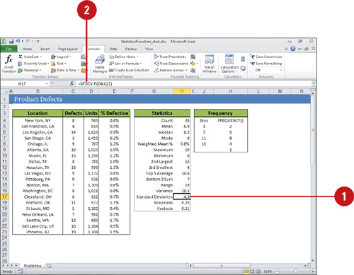
Using Statistical Functions
You can use statistical functions to help you perform analysis on a group of numbers. You can use formulas to find information, such as MAX or MIN (maximum or minimum value in a list), MEDIAN (median of given numbers), COUNT (number of items in a list), STDEV.S (standard deviation based on a sample) (New!), STDEV.P (standard deviation based on the entire population) (New!), SKEW (skewness of the distribution), or KURT (kurtosis of a data set).
Use Statistical Functions
![]() Click the cell where you want to place the function.
Click the cell where you want to place the function.
![]() Type = (equal sign), type a text function, specify the argument for the selected function, and then press Enter.
Type = (equal sign), type a text function, specify the argument for the selected function, and then press Enter.
Some syntax examples include:
![]() =MAX(number1, number2, ...)
=MAX(number1, number2, ...)
![]() =MIN(number1, number2, . . .)
=MIN(number1, number2, . . .)
![]() =MEDIAN(number1, number2, . . .)
=MEDIAN(number1, number2, . . .)
![]() =COUNT(value1, value2, ...)
=COUNT(value1, value2, ...)
![]() =STDEV.S(number1, number2, ...)
=STDEV.S(number1, number2, ...)
![]() =STDEV.P(number1, number2, ...)
=STDEV.P(number1, number2, ...)
![]() =SKEW(number1, number2, ...)
=SKEW(number1, number2, ...)
![]() =KURT(number1, number2, ...)
=KURT(number1, number2, ...)
Or click the Formulas tab, click the More Functions button, point to Statistical, click a function, specify the function arguments, and then click OK.
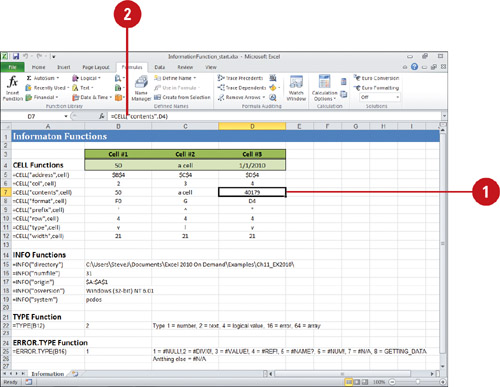
Using Information Functions
You can use information functions to help you determine the type of information in a cell or display information about formatting, location, or contents of a cell. The following information functions return TRUE when the function is valid: ISBLANK, ISERR, ISERROR, ISEVEN, ISLOGICAL, ISNA, ISNONTEXT, ISNUMBER, ISODD, ISREF, and ISTEXT. The other main information functions are CELL, INFO, TYPE, and ERROR.TYPE, which display information about the cell contents.
Use Information Functions
![]() Click the cell where you want to place the function.
Click the cell where you want to place the function.
![]() Type = (equal sign), type a text function, specify the argument for the selected function, and then press Enter.
Type = (equal sign), type a text function, specify the argument for the selected function, and then press Enter.
Some syntax examples include:
![]() =CELL(“contents”, cell)
=CELL(“contents”, cell)
![]() =INFO(“directory”)
=INFO(“directory”)
![]() =TYPE(cell)
=TYPE(cell)
![]() =ERROR.TYPE (error_val)
=ERROR.TYPE (error_val)
![]() =IF(ISERROR(A1, “an error occurred.”, A1 * 2)
=IF(ISERROR(A1, “an error occurred.”, A1 * 2)
Or click the Formulas tab, click the More Functions button, point to Information, click a function, specify the function arguments, and then click OK.
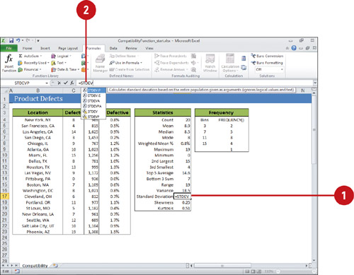
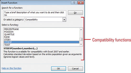
Using Compatibility Functions
Excel has replaced several functions with new functions that provide improved accuracy and whose names better reflect their usage (New!). For example, STDEVP has been replaced with STDEV.P. If you want to use an older version of a function for backwards compatibility in order to share your worksheets with those who do not have Excel 2010, you can use the Compatibility menu on the Formulas tab or the Compatibility option in the Insert Function dialog box to display and select the old function you want. When you enter a function, Formula AutoComplete lists both renamed and compatibility functions (New!). If compatibility is not an issue, you can use the new functions, which are available in the different function categories. Before you save a workbook in an earlier version of Excel, you should use the Compatibility Checker to determine whether new functions are used, so you can change them.
Use Compatibility Functions
![]() Click the cell where you want to place the function.
Click the cell where you want to place the function.
![]() Type = (equal sign), type a text function, specify the argument for the selected function, and then press Enter.
Type = (equal sign), type a text function, specify the argument for the selected function, and then press Enter.
Some syntax examples include:
![]() =STDEV.S(number1, number2, ...)
=STDEV.S(number1, number2, ...)
![]() =STDEV.P(number1, number2, ...)
=STDEV.P(number1, number2, ...)
Or click the Formulas tab, click the More Functions button, point to Compatibility, click a function, specify the function arguments, and then click OK.
Or click the Formulas tab, click the Insert Function button, click the Category list arrow, click Compatibility, click a function, click OK, specify the function arguments, and then click OK.