3 Working with Formulas and Functions
Introduction
Once you enter data in a worksheet, you’ll want to add formulas to perform calculations. Microsoft Excel can help you get the results you need. Formulas can be very basic entries to more complex ones. The difficulty of the formula depends on the complexity of the result you want from your data. For instance, if you are simply looking to total this months sales, then the formula would add your sales number and provide the result. However, if you were looking to show this months sales, greater than $100.00 with repeat customers, you would take a bit more time to design the formula.
Because Microsoft Excel automatically recalculates formulas, your worksheets remain accurate and up-to-date no matter how often you change the data. Using absolute cell references anchors formulas to a specific cell. Excel provides numerous built-in functions to add to your worksheet calculations. Functions, such as AVERAGE or SUM, allow you to perform a quick formula calculation.
Another way to make your formulas easier to understand is by using name ranges in them. Name ranges—a group of selected cells named as a range—can help you understand your more complicated formulas. It is a lot easier to read a formula that uses name ranges, then to look at the formula and try to decipher it. Excel offers a tool to audit your worksheet. Looking at the “flow” of your formula greatly reduces errors in the calculation. You can see how your formula is built, one level at a time through a series of arrows that point out where the formula is pulling data from. As you develop your formula, you can make corrections to it.
Understanding Formulas
Introduction
A formula calculates values to return a result. On an Excel worksheet, you can create a formula using constant values (such as 147 or $10.00), operators (shown in the table), references, and functions. An Excel formula always begins with the equal sign (=).
A constant is a number or text value that is not calculated, such as the number 147, the text “Total Profits” and the date 7/22/2010. On the other hand, an expression is a value that is not a constant. Constants remain the same until you or the system change them. An operator performs a calculation, such as + (plus sign) or - (minus sign). A cell reference is a cell address that returns the value in a cell. For example, A1 (column A and row 1) returns the value in cell A1 (see table below).

A function performs predefined calculations using specific values, called arguments. For example, the function SUM(B1:B10) returns the sum of cells B1 through B10. An argument can be numbers, text, logical values such as TRUE or FALSE, arrays, error values such as #NA, or cell references. Arguments can also be constants, formulas, or other functions, known as nested functions. A function starts with the equal sign (=), followed by the function name, an opening parenthesis, the arguments for the function separated by commas, and a closing parenthesis. For example, the function, AVERAGE(A1:A10, B1:B10), returns a number with the average for the contents of cells A1 through A10 and B1 through B10. As you type a function, a ToolTip appears with the structure and arguments needed to complete the function. You can also use the Insert Function dialog box to help you add a function to a formula.
Perform Calculations
By default, every time you make a change to a value, formula, or name, Excel performs a calculation. To change the way Excel performs calculations, click the Formulas tab, click the Calculation Options button, and then click the option you want: Automatic, Automatic Except Data Tables, or Manual. To manually recalculate all open workbooks, click the Calculate Now button (or press F9). To recalculate the active worksheet, click the Calculate Sheet button (or press Shift+F9).
Precedence Order
Formulas perform calculations from left to right, according to a specific order for each operator. Formulas containing more than one operator follow precedence order: exponentiation, multiplication and division, and then addition and subtraction. So, in the formula 2 + 5 * 7, Excel performs multiplication first and addition next for a result of 37. Excel calculates operations within parentheses first. The result of the formula (2 + 5) * 7 is 49.

Creating a Simple Formula
A formula calculates values to return a result. On an Excel worksheet, you can create a formula using values (such as 147 or $10.00), arithmetic operators (shown in the table), and cell references. An Excel formula always begins with the equal sign (=). The equal sign, when entered, automatically formats the cell as a formula entry. The best way to start a formula is to have an argument. An argument is the cell references or values in a formula that contribute to the result. Each function uses function-specific arguments, which may include numeric values, text values, cell references, ranges of cells, and so on. To accommodate long, complex formulas, you can resize the formula bar to prevent formulas from covering other data in your worksheet. By default, only formula results are displayed in a cell, but you can change the view of the worksheet to display formulas instead of results.
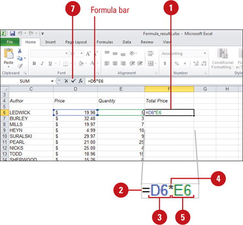
Enter a Formula
![]() Click the cell where you want to enter a formula.
Click the cell where you want to enter a formula.
![]() Type = (an equal sign). If you do not begin with an equal sign, Excel will display, not calculate, the information you type.
Type = (an equal sign). If you do not begin with an equal sign, Excel will display, not calculate, the information you type.
![]() Enter the first argument. An argument can be a number or a cell reference.
Enter the first argument. An argument can be a number or a cell reference.
TIMESAVER To avoid typing mistakes, click a cell to insert its cell reference in a formula rather than typing its address.
![]() Enter an arithmetic operator.
Enter an arithmetic operator.
![]() Enter the next argument.
Enter the next argument.
![]() Repeat steps 4 and 5 as needed to complete the formula.
Repeat steps 4 and 5 as needed to complete the formula.
![]() Click the Enter button on the formula bar, or press Enter.
Click the Enter button on the formula bar, or press Enter.
Notice that the result of the formula appears in the cell (if you select the cell, the formula itself appears on the formula bar).
TIMESAVER To wrap text in a cell, press Alt+Enter, which manually inserts a line break.
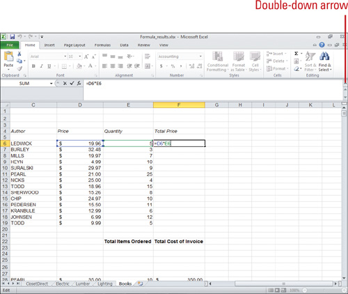
Resize the Formula Bar
![]() To switch between expanding the formula box to three or more lines or collapsing it to one line, click the double-down arrow at the end of the formula bar. You can also press Ctrl+Shift+U.
To switch between expanding the formula box to three or more lines or collapsing it to one line, click the double-down arrow at the end of the formula bar. You can also press Ctrl+Shift+U.
![]() To precisely adjust the height of the formula box, point to the bottom of the formula box until the pointer changes to a vertical double arrow, and then drag up or down, and then click the vertical double arrow or press Enter.
To precisely adjust the height of the formula box, point to the bottom of the formula box until the pointer changes to a vertical double arrow, and then drag up or down, and then click the vertical double arrow or press Enter.
![]() To automatically fit the formula box to the number of lines of text in the active cell, point to the formula box until the pointer changes to a vertical double arrow, and then double-click the vertical arrow.
To automatically fit the formula box to the number of lines of text in the active cell, point to the formula box until the pointer changes to a vertical double arrow, and then double-click the vertical arrow.
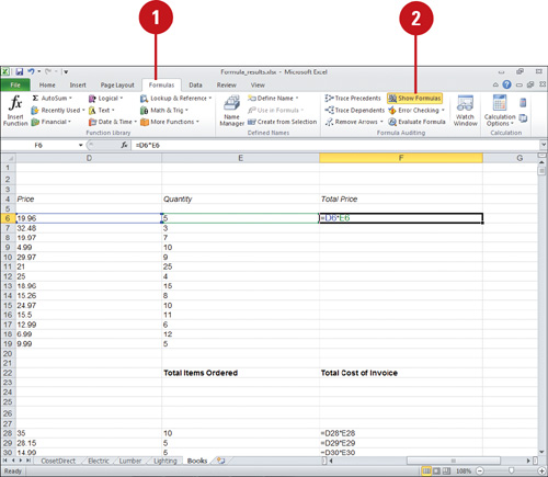
Display Formulas in Cells
![]() Click the Formulas tab.
Click the Formulas tab.
![]() Click the Show Formulas button.
Click the Show Formulas button.
TIMESAVER Press Ctrl+’.
![]() To turn off formula display, click the Show Formulas button again.
To turn off formula display, click the Show Formulas button again.
Creating a Formula Using Formula AutoComplete
To minimize typing and syntax errors, you can create and edit formulas with Formula AutoComplete. After you type an = (equal sign) and begin typing to start a formula, Excel displays a dynamic drop-down list of valid functions, arguments, defined names, table names, special item specifiers—including [(open bracket),, (comma),: (colon)—and text string that match the letters you type. An argument is the cell references or values in a formula that contribute to the result. Each function uses function-specific arguments, which may include numeric values, text values, cell references, ranges of cells, and so on.
Enter Items in a Formula Using Formula AutoComplete
![]() Click the cell where you want to enter a formula.
Click the cell where you want to enter a formula.
![]() Type = (an equal sign), and beginning letters or a display trigger to start Formula AutoComplete.
Type = (an equal sign), and beginning letters or a display trigger to start Formula AutoComplete.
For example, type su to display all value items, such as SUBTOTAL and SUM.
The text before the insertion point is used to display the values in the drop-down list.
![]() As you type, a drop-down scrollable list of valid items is displayed.
As you type, a drop-down scrollable list of valid items is displayed.
Icons represent the type of entry, such as a function or table reference, and a ScreenTip appears next to a selected item.
![]() To insert the selected item in the drop-down list into the formula, press Tab or double-click the item.
To insert the selected item in the drop-down list into the formula, press Tab or double-click the item.

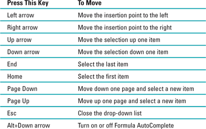
Use the Keyboard to Navigate
Using the keyboard, you can navigate the Formula AutoComplete drop-down list to quickly find the entry you want.
![]() Refer to the table for keyboard shortcuts for navigating the Formula AutoComplete drop-down list.
Refer to the table for keyboard shortcuts for navigating the Formula AutoComplete drop-down list.
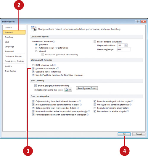
Turn on Formula AutoComplete
![]() Click the File tab, and then click Options.
Click the File tab, and then click Options.
![]() In the left pane, click Formulas.
In the left pane, click Formulas.
![]() Select the Formula AutoComplete check box.
Select the Formula AutoComplete check box.
![]() Click OK.
Click OK.
Editing a Formula
You can edit formulas just as you do other cell contents, using the formula bar or working in the cell. You can select, cut, copy, paste, delete, and format cells containing formulas just as you do cells containing labels or values. Using AutoFill, you can quickly copy formulas to adjacent cells. If you need to copy formulas to different parts of a worksheet, use the Paste command or Paste Options button.
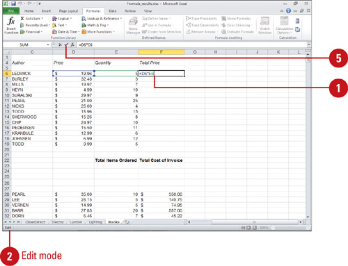
Edit a Formula Using the Formula Bar
![]() Select the cell that contains the formula you want to edit.
Select the cell that contains the formula you want to edit.
![]() Press F2 to change to Edit mode.
Press F2 to change to Edit mode.
![]() If necessary, use the Home, End, and arrow keys to position the insertion point within the cell contents.
If necessary, use the Home, End, and arrow keys to position the insertion point within the cell contents.
![]() Use any combination of Backspace and Delete to erase unwanted characters, and then type new characters as needed.
Use any combination of Backspace and Delete to erase unwanted characters, and then type new characters as needed.
![]() Click the Enter button on the formula bar, or press Enter.
Click the Enter button on the formula bar, or press Enter.
Copy a Formula Using AutoFill
![]() Select the cell that contains the formula you want to copy.
Select the cell that contains the formula you want to copy.
![]() Position the pointer (fill handle) on the lower-right corner of the selected cell.
Position the pointer (fill handle) on the lower-right corner of the selected cell.
![]() Drag the mouse down until the adjacent cells where you want the formula pasted are selected, and then release the mouse button.
Drag the mouse down until the adjacent cells where you want the formula pasted are selected, and then release the mouse button.

Copy and Paste a Formula
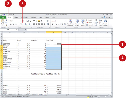
![]() Select the cell that contains the formula you want to copy.
Select the cell that contains the formula you want to copy.
![]() Click the Home tab.
Click the Home tab.
![]() Click the Copy button.
Click the Copy button.
![]() Select one or more cells where you want to paste the formula.
Select one or more cells where you want to paste the formula.
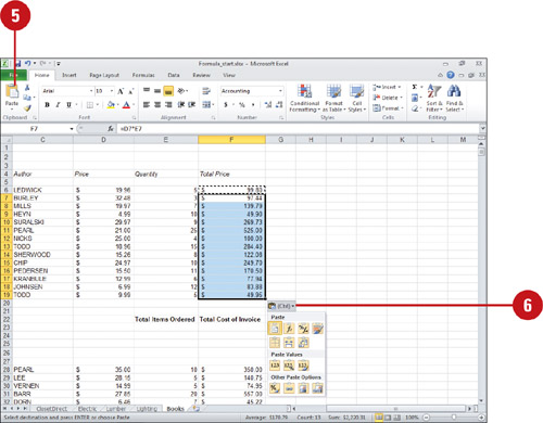
![]() Click the Paste button or click the Paste button arrow, point to an option to display a live preview (New!) of the paste, and then click to paste the item.
Click the Paste button or click the Paste button arrow, point to an option to display a live preview (New!) of the paste, and then click to paste the item.
![]() Click the Paste Options button, point to an option for the live preview (New!), and then select the option you want.
Click the Paste Options button, point to an option for the live preview (New!), and then select the option you want.
If you don’t want to paste this selection anywhere else, press Esc to remove the marquee.
Understanding Cell Referencing
Each cell, the intersection of a column and row on a worksheet, has a unique address, or cell reference, based on its column letter and row number. For example, the cell reference for the intersection of column D and row 4 is D4.
Cell References in Formulas
The simplest formula refers to a cell. If you want one cell to contain the same value as another cell, type an equal sign followed by the cell reference, such as =D4. The cell that contains the formula is known as a dependent cell because its value depends on the value in another cell. Whenever the cell that the formula refers to changes, the cell that contains the formula also changes.
Depending on your task, you can use relative cell references, which are references to cells relative to the position of the formula, absolute cell references, which are cell references that always refer to cells in a specific location, or mixed cell references, which use a combination of relative and absolute column and row references. If you use macros, the R1C1 cell references make it easy to compute row and column positions.
Relative Cell References
When you copy and paste or move a formula that uses relative references, the references in the formula change to reflect cells that are in the same relative position to the formula. The formula is the same, but it uses the new cells in its calculation. Relative addressing eliminates the tedium of creating new formulas for each row or column in a worksheet filled with repetitive information.
Absolute Cell References
If you don’t want a cell reference to change when you copy a formula, make it an absolute reference by typing a dollar sign ($) before each part of the reference that you don’t want to change. For example, $A$1 always refers to cell A1. If you copy or fill the formula down columns or across rows, the absolute reference doesn’t change. You can add a $ before the column letter and the row number. To ensure accuracy and simplify updates, enter constant values (such as tax rates, hourly rates, and so on) in a cell, and then use absolute references to them in formulas.
Mixed Cell References
A mixed reference is either an absolute row and relative column or absolute column and relative row. You add the $ before the column letter to create an absolute column or before the row number to create an absolute row. For example, $A1 is absolute for column A and relative for row 1, and A$1 is absolute for row 1 and relative for column A. If you copy or fill the formula across rows or down columns, the relative references adjust, and the absolute ones don’t adjust.
3-D References
3-D references allow you to analyze data in the same cell or range of cells on multiple worksheets within a workbook. A 3-D reference includes the cell or range reference, preceded by a range of worksheet names. For example, =AVERAGE(Sheet1:Sheet4!A1) returns the average for all the values contained in cell A1 on all the worksheets between and including Sheet 1 and Sheet 4.
Using Absolute Cell References
When you want a formula to consistently refer to a particular cell, even if you copy or move the formula elsewhere on the worksheet, you need to use an absolute cell reference. An absolute cell reference is a cell address that contains a dollar sign ($) in the row or column coordinate, or both. When you enter a cell reference in a formula, Excel assumes it is a relative reference unless you change it to an absolute reference. If you want part of a formula to remain a relative reference, remove the dollar sign that appears before the column letter or row number.
Create an Absolute Reference
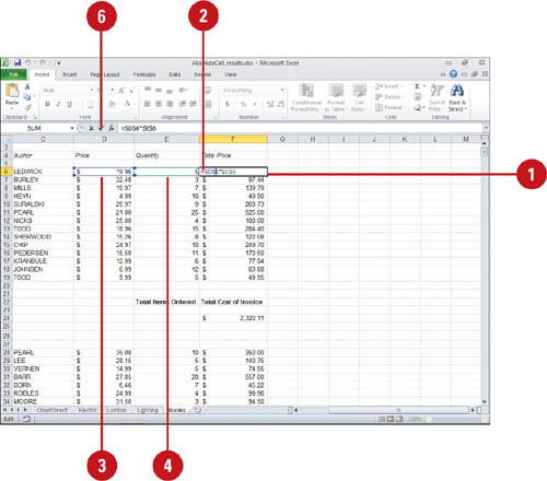
![]() Click a cell where you want to enter a formula.
Click a cell where you want to enter a formula.
![]() Type = (an equal sign) to begin the formula.
Type = (an equal sign) to begin the formula.
![]() Select a cell, and then type an arithmetic operator (+, -, *, or /).
Select a cell, and then type an arithmetic operator (+, -, *, or /).
![]() Select another cell, and then press the F4 key to make that cell reference absolute.
Select another cell, and then press the F4 key to make that cell reference absolute.
You can continue to press F4 to have Excel cycle through the different reference types.
![]() If necessary, continue entering the formula.
If necessary, continue entering the formula.
![]() Click the Enter button on the formula bar, or press Enter.
Click the Enter button on the formula bar, or press Enter.

Using Mixed Cell References
A mixed cell reference is either an absolute column and relative row or absolute row and relative column. When you add the $ before the column letter you create an absolute column or before the row number you create an absolute row. For example, $A1 is absolute for column A and relative for row 1, and A$1 is absolute for row 1 and relative for column A. If you copy or fill the formula across rows or down columns, the relative references adjust, and the absolute ones don’t adjust.
Create a Mixed Reference
![]() Click a cell where you want to enter a formula.
Click a cell where you want to enter a formula.
![]() Type = (an equal sign) to begin the formula.
Type = (an equal sign) to begin the formula.
![]() Select the cells you want to use and then complete the formula.
Select the cells you want to use and then complete the formula.
![]() Click the insertion point in the formula bar, and then type $ before the column or row you want to make absolute.
Click the insertion point in the formula bar, and then type $ before the column or row you want to make absolute.
![]() Click the Enter button on the formula bar, or press Enter.
Click the Enter button on the formula bar, or press Enter.


Using 3-D Cell References
If you want to analyze data in the same cell or range of cells on multiple worksheets within a workbook, use a mixed 3-D reference. For example, =SUM(Sheet3:Sheet6!A1:A10) returns the sum for all the values contained in the range of cells A1 through A10 on all the worksheets between and including Sheet 3 and Sheet 6. 3-D references work with the following functions: AVERAGE, AVERAGEA, COUNT, COUNTA, MAX, MAXA, MIN, MINA, PRODUCT, STDEV, STDEVA, STDE-VPA, VAR, VARA, VARP, and VARPA. However, 3-D references cannot be used with array formulas, the intersection operator (a single space), or the implicit intersection. If you move, insert, or copy sheets between the ones included in the range, Excel adds the values from the sheets in the calculations. If you move or remove sheets between the ones included in the range, Excel removes the values from the calculation.
Create a 3-D Cell Reference
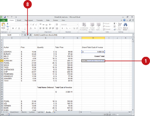
![]() Click a cell where you want to enter a formula.
Click a cell where you want to enter a formula.
![]() Type = (an equal sign) to begin the formula.
Type = (an equal sign) to begin the formula.
![]() Type the function you want to use followed by a ((left bracket).
Type the function you want to use followed by a ((left bracket).
![]() Type the first worksheet name, followed by a : (colon), and then the last worksheet name in the range.
Type the first worksheet name, followed by a : (colon), and then the last worksheet name in the range.
![]() Type ! (exclamation).
Type ! (exclamation).
![]() Type or select the cell or cell range you want to use in the function.
Type or select the cell or cell range you want to use in the function.
![]() Type ) (right bracket).
Type ) (right bracket).
![]() Click the Enter button on the formula bar, or press Enter.
Click the Enter button on the formula bar, or press Enter.

Naming Cells and Ranges
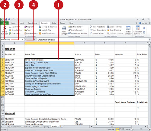
To make working with ranges easier, Excel allows you to name them. The name BookTitle, for example, is easier to remember than the range reference B6:B21. Named ranges can be used to navigate large worksheets. Named ranges can also be used in formulas instead of typing or pointing to specific cells. When you name a cell or range, Excel uses an absolute reference for the name by default, which is almost always what you want. You can see the absolute reference in the Refers to box in the New Name dialog box. There are two types of names you can create and use: defined name and table name. A defined name represents a cell, a range of cells, formula or constant, while a table name represents an Excel table, which is a collection of data stored in records (rows) and fields (columns). You can define a name for use in a worksheet or an entire workbook, also known as scope. To accommodate long names, you can resize the name box in the formula bar. The worksheet and formula bar work together to avoid overlapping content.
Name a Cell or Range Using the Name Box
![]() Select the cell or range, or nonadjacent selections you want to name.
Select the cell or range, or nonadjacent selections you want to name.
![]() Click the Name box on the formula bar.
Click the Name box on the formula bar.
![]() Type a name for the range.
Type a name for the range.
A range name can include up to 255 characters, uppercase or lowercase letters (not case sensitive), numbers, and punctuation, but no spaces or cell references.
By default, names use absolute cell references.
![]() To adjust the width of the Name box, point between the Name box and the Formula box until the pointer changes to a horizontal double arrow, and then drag left or right.
To adjust the width of the Name box, point between the Name box and the Formula box until the pointer changes to a horizontal double arrow, and then drag left or right.
![]() Press Enter. The range name will appear in the Name box whenever you select the range in the workbook.
Press Enter. The range name will appear in the Name box whenever you select the range in the workbook.
Let Excel Name a Cell or Range
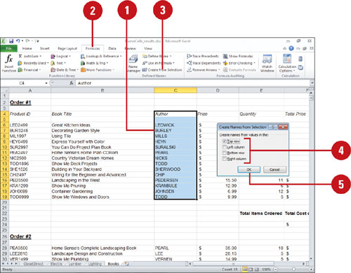
![]() Select the cells, including the column or row header, you want to name.
Select the cells, including the column or row header, you want to name.
![]() Click the Formulas tab.
Click the Formulas tab.
![]() Click the Create from Selection button.
Click the Create from Selection button.
![]() Select the check box with the position of the labels in relation to the cells.
Select the check box with the position of the labels in relation to the cells.
Excel automatically tries to determine the position of the labels, so you might not have to change any options.
![]() Click OK.
Click OK.
Name a Cell or Range Using the New Name Dialog Box
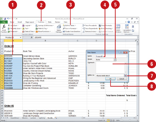
![]() Select the cell or range, or nonadjacent selections you want to name.
Select the cell or range, or nonadjacent selections you want to name.
![]() Click the Formulas tab.
Click the Formulas tab.
![]() Click the Define Name button.
Click the Define Name button.
![]() Type a name for the reference.
Type a name for the reference.
![]() Click the Scope list arrow, and then click Workbook or a specific worksheet.
Click the Scope list arrow, and then click Workbook or a specific worksheet.
![]() If you want, type a description of the name.
If you want, type a description of the name.
The current selection appears in the Refer to box.
![]() Click the Collapse Dialog button, select different cells and click the Expand Dialog button, or type = (equal sign) followed by a constant value or a formula.
Click the Collapse Dialog button, select different cells and click the Expand Dialog button, or type = (equal sign) followed by a constant value or a formula.
![]() Click OK.
Click OK.
Entering Named Cells and Ranges
After you define a named cell or range, you can enter a name by typing, using the Name box, using Formula AutoComplete, or selecting from the Use in Formula command. As you begin to type a name in a formula, Formula AutoComplete displays valid matches in a drop-down list, which you can select and insert into a formula. You can also select a name from a list of available from the Use in Formula command. If you have already entered a cell or range address in a formula or function, you can apply a name to the address instead of re-creating it.
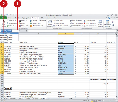
Enter a Named Cell or Range Using the Name Box
![]() Click the Name box list arrow on the formula bar.
Click the Name box list arrow on the formula bar.
![]() Click the name of the cell or range you want to use.
Click the name of the cell or range you want to use.
The range name appears in the Name box, and all cells included in the range are highlighted on the worksheet.
Enter a Named Cell or Range Using Formula AutoComplete
![]() Type = (equal sign) to start a formula, and then type the first letter of the name.
Type = (equal sign) to start a formula, and then type the first letter of the name.
![]() To insert a name, type the first letter of the name to display it in the Formula AutoComplete dropdown list.
To insert a name, type the first letter of the name to display it in the Formula AutoComplete dropdown list.
![]() Scroll down the list, if necessary, to select the name you want, and then press Tab or double-click the name to insert it.
Scroll down the list, if necessary, to select the name you want, and then press Tab or double-click the name to insert it.
Enter a Named Cell or Range from the Use in Formula Command
![]() Type = (equal sign) to start a formula.
Type = (equal sign) to start a formula.
![]() Click the Formulas tab.
Click the Formulas tab.
![]() When you want to insert a name, click the Use in Formula button.
When you want to insert a name, click the Use in Formula button.
![]() Use one of the following menu options:
Use one of the following menu options:
![]() Click the name you want to use.
Click the name you want to use.
![]() Click Paste Names, select a name, and then click OK.
Click Paste Names, select a name, and then click OK.

Apply a Name to a Cell or Range Address
![]() Select the cells in which you want to apply a name.
Select the cells in which you want to apply a name.
![]() Click the Formulas tab.
Click the Formulas tab.
![]() Click the Define Name button arrow, and then click Apply Names.
Click the Define Name button arrow, and then click Apply Names.
![]() Click the name you want to apply.
Click the name you want to apply.
![]() Click OK.
Click OK.

Managing Names
The Name Manager makes it easy to work with all the defined names and table names in a workbook from one location. You can display the value and reference of a name, specify the scope—either worksheet or workbook level—of a name, find names with errors, and view or edit name descriptions. In addition, you can add, change, or delete names, and sort and filter the names list. You can also use table column header names in formulas instead of cell references.
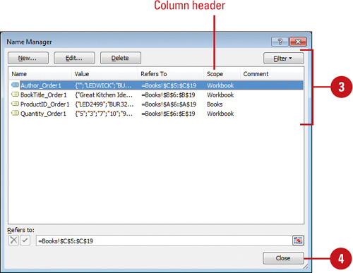
Organize and View Names
![]() Click the Formulas tab.
Click the Formulas tab.
![]() Click the Name Manager button.
Click the Name Manager button.
TROUBLE? You cannot use the Name Manager dialog box while you’re editing a cell. The Name Manager doesn’t display names defined in VBA or hidden names.
![]() Use one of the following menu options:
Use one of the following menu options:
![]() Resize columns. Double-click the right side of the column header to automatically size the column to fit the largest value in that column.
Resize columns. Double-click the right side of the column header to automatically size the column to fit the largest value in that column.
![]() Sort names. Click the column header to sort the list of names in ascending or descending order.
Sort names. Click the column header to sort the list of names in ascending or descending order.
![]() Filter names. Click the Filter button, and then select the filter command you want. See table for filter option details.
Filter names. Click the Filter button, and then select the filter command you want. See table for filter option details.
![]() Click Close.
Click Close.

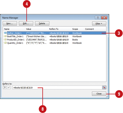
Change a Name
![]() Click the Formulas tab.
Click the Formulas tab.
![]() Click the Names Manager button.
Click the Names Manager button.
![]() Click the name you want to change.
Click the name you want to change.
![]() Click Edit.
Click Edit.
![]() Type a new name for the reference in the Name box.
Type a new name for the reference in the Name box.
![]() Change the reference. Enter a range or use the Collapse button to select one.
Change the reference. Enter a range or use the Collapse button to select one.
![]() Click OK.
Click OK.
![]() In the Refers to area, make any changes you want to the cell, formula, or constant represented by the name.
In the Refers to area, make any changes you want to the cell, formula, or constant represented by the name.
To cancel unwanted changes, click the Cancel button or press Esc, or to save changes, click the Commit buttonor press Enter.
![]() Click Close.
Click Close.

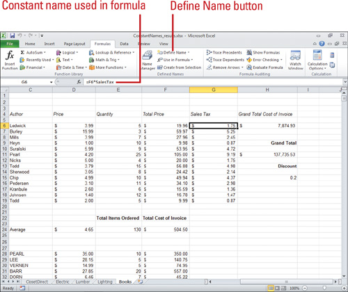
Simplifying a Formula with Ranges
You can simplify formulas by using ranges and range names. For example, if 12 cells on your worksheet contain monthly budget amounts, and you want to multiply each amount by 10%, you can insert one range address in a formula instead of inserting 12 different cell addresses, or you can insert a range name. Using a range name in a formula helps to identify what the formula does; the formula =TotalOrder*0.10, for example, is more meaningful than =SUM(F6:F19)*0.10.
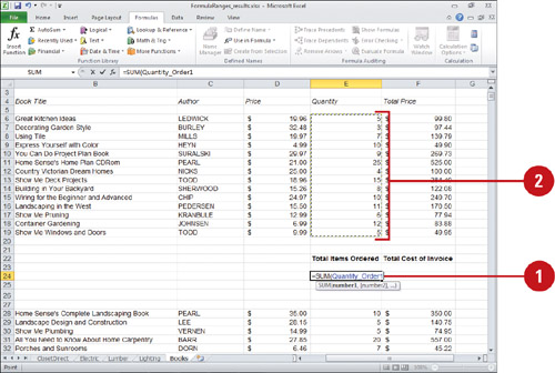
Use a Range in a Formula
![]() Put your cursor where you would like the formula. Type an equal sign (=) followed by the start of a formula, such as =SUM(.
Put your cursor where you would like the formula. Type an equal sign (=) followed by the start of a formula, such as =SUM(.
![]() Click the first cell of the range, and then drag to select the last cell in the range. Excel enters the range address for you.
Click the first cell of the range, and then drag to select the last cell in the range. Excel enters the range address for you.
![]() Complete the formula by entering a close parentheses, or another function, and then click the Enter button.
Complete the formula by entering a close parentheses, or another function, and then click the Enter button.
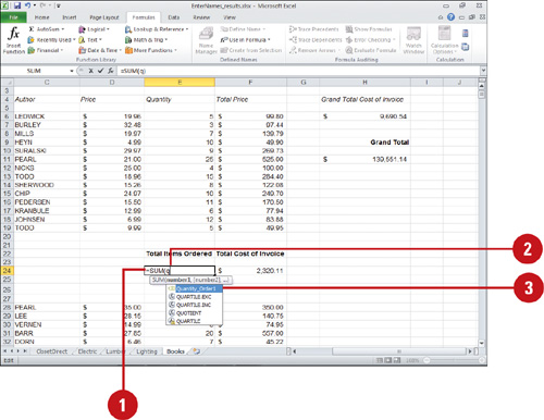
Use a Range Name in a Formula
![]() Put your cursor where you would like the formula. Type an equal sign (=) followed by the start of a formula, such as =SUM(.
Put your cursor where you would like the formula. Type an equal sign (=) followed by the start of a formula, such as =SUM(.
![]() Press F3 to display a list of named ranges.
Press F3 to display a list of named ranges.
![]() You can also click the Use in Formula button on the Formulas tab, and then click Paste.
You can also click the Use in Formula button on the Formulas tab, and then click Paste.
![]() Click the name of the range you want to insert.
Click the name of the range you want to insert.
![]() Click OK.
Click OK.
![]() Complete the formula by entering a close parentheses, or another function, and then click the Enter button.
Complete the formula by entering a close parentheses, or another function, and then click the Enter button.

Displaying Calculations with the Status Bar
You can simplify your work using the Status bar calculations when you don’t want to insert a formula, but you want to quickly see the results of a simple calculation. The Status bar automatically displays the sum, average, maximum, minimum, or count of the selected values. The Status bar results do not appear on the worksheet when printed but are useful for giving you quick answers while you work. If a cell contains text, it’s ignored, except when you select the Count option.
Calculate a Range Automatically
![]() Select the range of cells you want to calculate.
Select the range of cells you want to calculate.
The sum, average, and count of the selected cells appears on the status bar by default.
![]() If you want to change the type of calculations that appear on the Status bar, right-click anywhere on the Status bar to display a shortcut menu.
If you want to change the type of calculations that appear on the Status bar, right-click anywhere on the Status bar to display a shortcut menu.
The shortcut menu displays all the available status information you can track. The right side of the menu displays the current values for the different calculations.
![]() Click to toggle (on or off) the available types of calculations.
Click to toggle (on or off) the available types of calculations.
![]() Average
Average
![]() Count
Count
![]() Numerical Count
Numerical Count
![]() Minimum
Minimum
![]() Maximum
Maximum
![]() Sum
Sum

Calculating Totals with AutoSum
A range of cells can easily be added using the AutoSum button on the Formulas tab. AutoSum suggests the range to sum, although this range can be changed if it’s incorrect. AutoSum looks at all of the data that is consecutively entered, and when it sees an empty cell, that is where the AutoSum stops. You can also use AutoSum to perform other calculations, such as AVERAGE, COUNT, MAX, and MIN. Subtotals can be calculated for data ranges using the Subtotals dialog box. This dialog box lets you select where the subtotals occur, as well as the function type.
Calculate Totals with AutoSum
![]() Click the cell where you want to display the calculation.
Click the cell where you want to display the calculation.
![]() To sum with a range of numbers, select the range of cells you want.
To sum with a range of numbers, select the range of cells you want.
![]() To sum with only some of the numbers in a range, select the cells or range you want using the Ctrl key. Excel inserts the sum in the first empty cell below the selected range.
To sum with only some of the numbers in a range, select the cells or range you want using the Ctrl key. Excel inserts the sum in the first empty cell below the selected range.
![]() To sum both across and down a table of number, select the range of cells with an additional column to the right and a row at the bottom.
To sum both across and down a table of number, select the range of cells with an additional column to the right and a row at the bottom.
![]() Click the Formulas tab.
Click the Formulas tab.
![]() Click the AutoSum button.
Click the AutoSum button.
TIMESAVER Press Alt+= to access the AutoSum command.
![]() Click the Enter button on the formula bar, or press Enter.
Click the Enter button on the formula bar, or press Enter.

Calculate with Extended AutoSum
![]() Click the cell where you want to display the calculation.
Click the cell where you want to display the calculation.
![]() Click the Formulas tab.
Click the Formulas tab.
![]() Click the AutoSum button arrow.
Click the AutoSum button arrow.
![]() Click the function you want to use, such as AVERAGE, COUNT, MAX, and MIN.
Click the function you want to use, such as AVERAGE, COUNT, MAX, and MIN.
![]() Press Enter to accept the range selected.
Press Enter to accept the range selected.

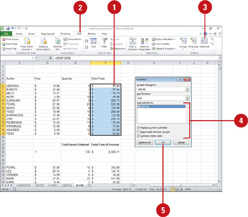
Calculate Subtotals and Totals
![]() Click anywhere within the data to be subtotaled.
Click anywhere within the data to be subtotaled.
![]() Click the Data tab.
Click the Data tab.
![]() Click the Subtotal button.
Click the Subtotal button.
If a message box appears, read the message, and then click the appropriate button.
![]() Select the appropriate check boxes to specify how the data is subtotaled.
Select the appropriate check boxes to specify how the data is subtotaled.
![]() Click OK.
Click OK.
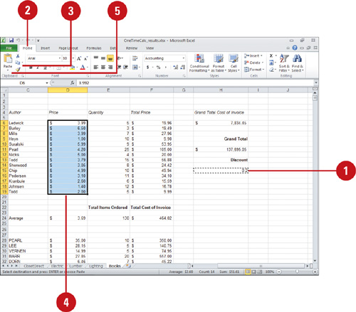
Performing One Time Calculations
Sometimes you may want to perform simple calculations, such as dividing each value in a range by 4, without having to take the time to use a formula. You can use the Paste Special command to perform simple mathematical operations, such as Add, Subtract, Multiply, and Divide. If you want to perform a more complex function, you can create a temporary formula to accomplish a one-time task. For example, if you want to display a list of names in proper case with only the first letter of each name in uppercase, you can use the Proper function.
Perform One Time Simple Calculations without Using a Formula
![]() Select an empty cell, and then enter the number you want to use in a calculation.
Select an empty cell, and then enter the number you want to use in a calculation.
![]() Click the Home tab.
Click the Home tab.
![]() Click the Copy button.
Click the Copy button.
![]() Select the range you want to use in the calculation.
Select the range you want to use in the calculation.
![]() Click the Paste button arrow, and then click Paste Special.
Click the Paste button arrow, and then click Paste Special.
![]() Click the operation option you want to use: Add, Subtract, Multiply, or Divide.
Click the operation option you want to use: Add, Subtract, Multiply, or Divide.
![]() Click OK.
Click OK.
![]() Press Esc to cancel Copy mode.
Press Esc to cancel Copy mode.
The operation is applied to the contents of each cell in the range. The formula in each cell is changed to include the new operation.

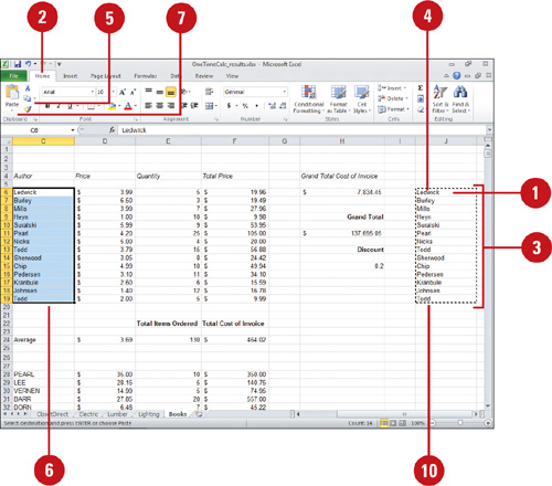
Perform One Time Calculations Using a Formula
![]() Create a temporary formula in an unused cell, typically a column out of the way. Select an empty cell at the top, type = (equal sign), and then type a function, such as Proper().
Create a temporary formula in an unused cell, typically a column out of the way. Select an empty cell at the top, type = (equal sign), and then type a function, such as Proper().
![]() Click the Home tab.
Click the Home tab.
![]() If you want to change a range of data, use the fill down handle to copy the formula to unused cells.
If you want to change a range of data, use the fill down handle to copy the formula to unused cells.
![]() Select the cell or range with the formula.
Select the cell or range with the formula.
![]() Click the Copy button.
Click the Copy button.
![]() Select the cell you want to change the contents with the formula.
Select the cell you want to change the contents with the formula.
![]() Click the Paste button arrow, and then click Paste Special.
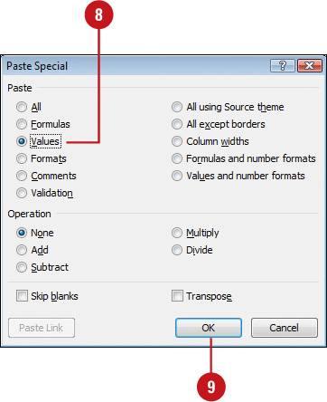
Click the Paste button arrow, and then click Paste Special.
![]() Click the Values option.
Click the Values option.
![]() Click OK.
Click OK.
The original data is replaced with the changed data.
![]() When you’re done with the temporary formulas, select the cells, and delete them.
When you’re done with the temporary formulas, select the cells, and delete them.
Converting Formulas and Values
If you have a range of cells that contain formulas, you can convert the cells to values only. This is useful when you have a range of cells that you don’t want to change anymore. You use the Paste Special command to paste the contents of the selected range back into place as a value instead of a formula. If you’re working with an input form in Excel, you probably need to delete values, but keep the formulas. You can do it with the help of the Go To Special dialog box.
Convert a Formula to a Value
![]() Select the range of cells with formulas you want to convert to values.
Select the range of cells with formulas you want to convert to values.
![]() Click the Home tab.
Click the Home tab.
![]() Click the Copy button.
Click the Copy button.
![]() Click the Paste button arrow, and then click Paste Special.
Click the Paste button arrow, and then click Paste Special.
![]() Click the Values option.
Click the Values option.
![]() Click OK.
Click OK.
![]() Press Esc to cancel Copy mode.
Press Esc to cancel Copy mode.

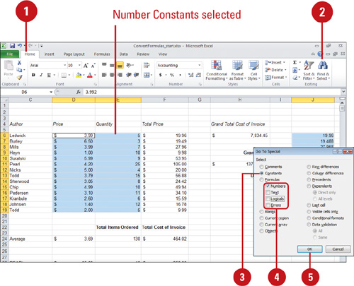
Delete Values and Keep Formulas
![]() Click the Home tab.
Click the Home tab.
![]() Click the Find & Select button, and then click Go To Special.
Click the Find & Select button, and then click Go To Special.
![]() Click the Constants option.
Click the Constants option.
![]() Select the Numbers check box, and then clear the other check boxes under Formula.
Select the Numbers check box, and then clear the other check boxes under Formula.
![]() Click OK.
Click OK.
![]() Press Delete to remove the selected values.
Press Delete to remove the selected values.
Correcting Calculation Errors
When Excel finds a possible error in a calculation, it displays a green triangle in the upper left corner of the cell. If Excel can’t complete a calculation it displays an error message, such as “#DIV/0!” or “#NAME?. You can use the Error Options button to help you fix the problem. In a complex worksheet, it can be difficult to understand the relationships between cells and formulas. Auditing tools enable you to clearly determine these relationships. When the Auditing feature is turned on, it uses a series of arrows to show you which cells are part of which formulas. When you use the auditing tools, tracer arrows point out cells that provide data to formulas and the cells that contain formulas that refer to the cells. A box is drawn around the range of cells that provide data to formulas.
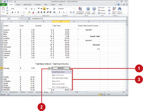
Review and Correct Errors
![]() Select a cell that contains a green triangle in the upper left corner.
Select a cell that contains a green triangle in the upper left corner.
![]() Click the Error Options button.
Click the Error Options button.
![]() Click one of the troubleshooting options (menu options vary depending on the error).
Click one of the troubleshooting options (menu options vary depending on the error).
![]() To have Excel fix the error, click one of the available options specific to the error.
To have Excel fix the error, click one of the available options specific to the error.
![]() To find out more about an error, click Help on this Error.
To find out more about an error, click Help on this Error.
![]() To evaluate the formula, click Show Calculation Steps.
To evaluate the formula, click Show Calculation Steps.
![]() To remove the error alert, click Ignore Error.
To remove the error alert, click Ignore Error.
![]() To fix the error manually, click Edit in Formula Bar.
To fix the error manually, click Edit in Formula Bar.
![]() To enable background error checking, specify an error color, or reset ignored errors, click Error Checking Options.
To enable background error checking, specify an error color, or reset ignored errors, click Error Checking Options.
Correcting Formulas
Excel has several tools to help you find and correct problems with formulas. One tool is the Watch window and another is the Error checker. The Watch window keeps track of cells and their formulas as you make changes to a worksheet. Excel uses an error checker in the same way Microsoft Word uses a grammar checker. The Error checker uses certain rules, such as using the wrong argument type, a number stored as text or an empty cell reference, to check for problems in formulas.
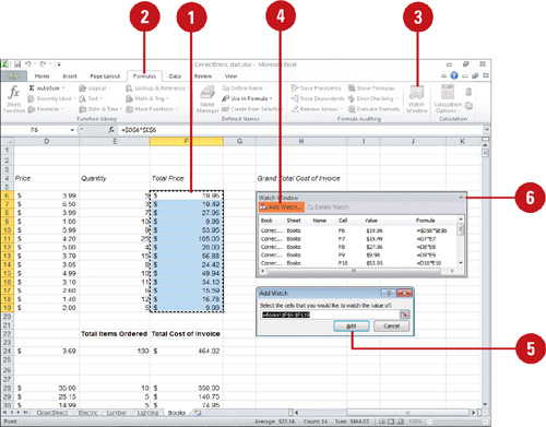
Watch Cells and Formulas
![]() Select the cells you want to watch.
Select the cells you want to watch.
![]() Click the Formulas tab.
Click the Formulas tab.
![]() Click the Watch Window button.
Click the Watch Window button.
![]() Click the Add Watch button on the Watch Window dialog box.
Click the Add Watch button on the Watch Window dialog box.
![]() Click Add.
Click Add.
![]() Click Close.
Click Close.
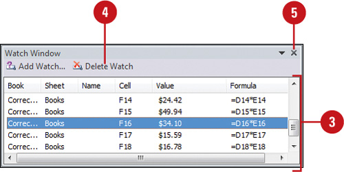
Remove Cells from the Watch Window
![]() Click the Formulas tab.
Click the Formulas tab.
![]() Click the Watch Window button.
Click the Watch Window button.
![]() Select the cells you want to delete. Use the Ctrl key to select multiple cells.
Select the cells you want to delete. Use the Ctrl key to select multiple cells.
![]() Click Delete Watch.
Click Delete Watch.
![]() Click Close.
Click Close.
Set Error Checking Options
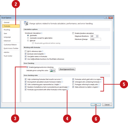
![]() Click the File tab, and then click Options.
Click the File tab, and then click Options.
![]() In the left pane, click Formulas.
In the left pane, click Formulas.
![]() Select the Enable background error checking check box.
Select the Enable background error checking check box.
![]() Point to the help icons at the end of the error checking rule options to display a ScreenTip describing the rule.
Point to the help icons at the end of the error checking rule options to display a ScreenTip describing the rule.
![]() Select the error checking rules check boxes you want to use.
Select the error checking rules check boxes you want to use.
![]() Click OK.
Click OK.
Correct Errors
![]() Open the worksheet where you want to check for errors.
Open the worksheet where you want to check for errors.
![]() Click the Formulas tab.
Click the Formulas tab.
![]() Click the Error Checking button.
Click the Error Checking button.
The error checker scans the worksheet for errors, generating the Error Checking dialog box every time it encounters an error.
![]() If necessary, click Resume.
If necessary, click Resume.
![]() Choose a button to correct or ignore the problem.
Choose a button to correct or ignore the problem.
![]() Help on this error.
Help on this error.
![]() Show Calculation Steps. Click Evaluate to see results.
Show Calculation Steps. Click Evaluate to see results.
![]() Ignore Error.
Ignore Error.
![]() Edit in Formula Bar.
Edit in Formula Bar.
![]() Previous or Next.
Previous or Next.
![]() If necessary, click Close.
If necessary, click Close.

Auditing a Worksheet
In a complex worksheet, it can be difficult to understand the relationships between cells and formulas. Auditing tools enable you to clearly determine these relationships. When the Auditing feature is turned on, it uses a series of arrows to show you which cells are part of which formulas. When you use the auditing tools, tracer arrows point out cells that provide data to formulas and the cells that contain formulas that refer to the cells. A box is drawn around the range of cells that provide data to formulas.
Trace Worksheet Relationships
![]() Click the Formulas tab.
Click the Formulas tab.
![]() Use any of the following options:
Use any of the following options:
![]() Click the Trace Precedents button to find cells that provide data to a formula.
Click the Trace Precedents button to find cells that provide data to a formula.
![]() Click the Trace Dependents button to find out which formulas refer to a cell.
Click the Trace Dependents button to find out which formulas refer to a cell.
![]() Click the Error Checking button arrow, and then click Trace Error tolocate the problem if a formula displays an error value, such as #DIV/0!.
Click the Error Checking button arrow, and then click Trace Error tolocate the problem if a formula displays an error value, such as #DIV/0!.
![]() Click the Remove Arrows button arrow, and then click Remove Precedent Arrows, Remove Dependent Arrows, or Remove All Arrows to remove precedent and dependent arrows.
Click the Remove Arrows button arrow, and then click Remove Precedent Arrows, Remove Dependent Arrows, or Remove All Arrows to remove precedent and dependent arrows.
![]() If necessary, click OK to locate the problem.
If necessary, click OK to locate the problem.

Locating Circular References
A circular reference occurs when a formula directly or indirectly refers to its own cell. This causes the formula to use its result in the calculation, which can create errors. When a workbook contains a circular reference, Excel cannot automatically perform calculations. You can use error checking in Excel to locate circular references in a formula, and then remove them. If you leave them in, Excel calculates each cell involved in the circular reference by using the results of the previous iteration. An iteration is a repeated recalculation until a specific numeric condition is met. By default, Excel stops calculating after 100 iterations or after all values in the circular reference change by less than 0.001 between iterations, unless you change the Excel option.
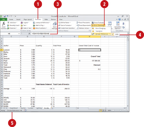
Locate a Circular Reference
![]() Click the Formulas tab.
Click the Formulas tab.
![]() Click the Error Checking button arrow, point to Circular References, and then click the first cell listed in the submenu.
Click the Error Checking button arrow, point to Circular References, and then click the first cell listed in the submenu.
![]() Review the formula cell.
Review the formula cell.
![]() If you cannot figure out if the cell is the cause of the circular reference, click the next cell in the Circular References submenu, if available.
If you cannot figure out if the cell is the cause of the circular reference, click the next cell in the Circular References submenu, if available.
![]() Continue to review and correct the circular reference until the status bar no longer displays the word “Circular.”
Continue to review and correct the circular reference until the status bar no longer displays the word “Circular.”
Performing Calculations Using Functions
Functions are predesigned formulas that save you the time and trouble of creating commonly used or complex equations. Excel includes hundreds of functions that you can use alone or in combination with other formulas or functions. Functions perform a variety of calculations, from adding, averaging, and counting to more complicated tasks, such as calculating the monthly payment amount of a loan. You can enter a function manually if you know its name and all the required arguments, or you can easily insert a function using AutoComplete, which helps you select a function and enter arguments with the correct format.
Enter a Function
![]() Click the cell where you want to enter the function.
Click the cell where you want to enter the function.
![]() Type = (an equal sign), type the name of the function, and then type ( (an opening parenthesis).
Type = (an equal sign), type the name of the function, and then type ( (an opening parenthesis).
As you type, you can scroll down the Formula AutoComplete list, select the function you want, and then press Tab.
![]() Type the argument or select the cell or range you want to insert in the function, and then type) (a closed parenthesis) to complete the function.
Type the argument or select the cell or range you want to insert in the function, and then type) (a closed parenthesis) to complete the function.
![]() Click the Enter button on the formula bar, or press Enter.
Click the Enter button on the formula bar, or press Enter.
Excel will automatically add the closing parenthesis to complete the function.


Creating Functions
Functions are predesigned formulas that save you the time and trouble of creating commonly used or complex equations. Trying to write a formula that calculates various pieces of data, such as calculating payments for an investment over a period of time at a certain rate, can be difficult and time-consuming. The Insert Function feature simplifies the process by organizing Excel’s built-in formulas, called functions, into categories so they are easy to find and use. A function defines all the necessary components (also called arguments) you need to produce a specific result; all you have to do is supply the values, cell references, and other variables. You can even combine one or more functions.
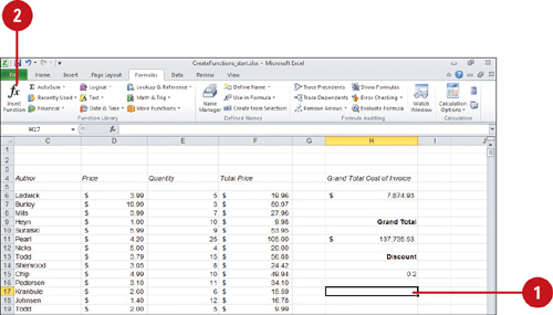
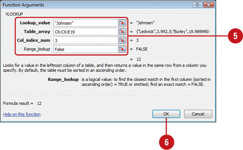
Enter a Function Using Insert Function
![]() Click the cell where you want to enter the function.
Click the cell where you want to enter the function.
![]() Click the Insert Function button on the Formula bar or click the Function Wizard button on the Formulas tab.
Click the Insert Function button on the Formula bar or click the Function Wizard button on the Formulas tab.
![]() Type a brief description that describes what you want to do in the Search for a function box, and then click Go.
Type a brief description that describes what you want to do in the Search for a function box, and then click Go.
![]() If necessary, click a function category you want to use.
If necessary, click a function category you want to use.
![]() Click the function you want to use.
Click the function you want to use.
![]() Click OK.
Click OK.
![]() Enter the cell addresses in the text boxes. Type them or click the Collapse Dialog button to the right of the text box, select the cell or range using your mouse, and then click the Expand Dialog button.
Enter the cell addresses in the text boxes. Type them or click the Collapse Dialog button to the right of the text box, select the cell or range using your mouse, and then click the Expand Dialog button.
![]() Click OK.
Click OK.

Creating Functions Using the Library
To make it easier to find the function you need for a specific use, Excel has organized functions into categories—such as Financial, Logical, Text, Date & Time, Lookup & Reference, Math & Trig, and other functions—on the Formulas tab. Functions—such as beta and chi-squared distributions—for the academic, engineering, and scientific community have been improved for more accuracy (New!). Some statistical functions have been renamed for consistency with the real world (New!). If you want to use an older version of a function for backwards compatibility with those who do not have Excel 2010, you can use the old functions on the Compatibility menu (New!) by using the More Functions button. After you use a function, Excel places it on the recently used list. When you insert a function from the Function Library, Excel inserts the function in the formula bar and opens a Function Argument dialog box, where you can enter or select the cells you want to use in the function.
Enter a Function Using the Function Library
![]() Click the cell where you want to enter the function.
Click the cell where you want to enter the function.
![]() Click the Formulas tab.
Click the Formulas tab.
![]() Type =(an equal sign).
Type =(an equal sign).
![]() Click the button (Financial, Logical, Text, Date & Time, Lookup & Reference, Math & Trig, More Functions, or Recently Used) from the Function Library with the type of function you want to use, click a submenu if necessary, and then click the function you want to insert into a formula.
Click the button (Financial, Logical, Text, Date & Time, Lookup & Reference, Math & Trig, More Functions, or Recently Used) from the Function Library with the type of function you want to use, click a submenu if necessary, and then click the function you want to insert into a formula.
Excel inserts the function you selected into the formula bar with a set of parenthesis, and opens the Function Arguments dialog box.
![]() Type the argument or select the cell or range you want to insert in the function.
Type the argument or select the cell or range you want to insert in the function.
You can click the Collapse Dialog button to the right of the text box, select the cell or range using your mouse, and then click the Expand Dialog button.
![]() Click OK.
Click OK.

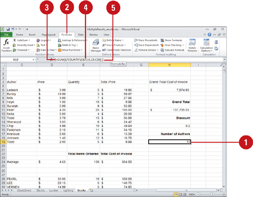
Calculating Multiple Results
An array formula can perform multiple calculations and then return either a single or multiple result. For example, when you want to count the number of distinct entries in a range, you can use an array formula, such as {=SUM(1/COUNTIF(range, range))}. You can also use an array formula to perform a two column lookup using the LOOKUP function. An array formula works on two or more sets of values, known as array arguments. Each argument must have the same number of rows and columns. You can create array formulas in the same way that you create other formulas, except you press Ctrl+Shift+Enter to enter the formula. When you enter an array formula, Excel inserts the formula between { } (brackets).
Create an Array Formula
![]() Click the cell where you want to enter the array formula.
Click the cell where you want to enter the array formula.
![]() Click the Formulas tab.
Click the Formulas tab.
![]() Type =(an equal sign).
Type =(an equal sign).
![]() Use any of the following methods to enter the formula you want.
Use any of the following methods to enter the formula you want.
![]() Type the function.
Type the function.
![]() Type and use Formula AutoComplete.
Type and use Formula AutoComplete.
![]() Use the Function Wizard.
Use the Function Wizard.
![]() Use button in the Function Library.
Use button in the Function Library.
![]() Press Ctrl+Shift+Enter.
Press Ctrl+Shift+Enter.
{ } (brackets) appear around the function to indicate it’s an array formula.
Using Nested Functions
A nested function uses a function as one of the arguments. Excel allows you to nest up to 64 levels of functions. Users typically create nested functions as part of a conditional formula. For example, IF (AVERAGE(B2:B10)>100, SUM(C2:G10),0). The AVERAGE and SUM functions are nested within the IF function. The structure of the IF function is IF(condition_test, if_true, if_false). You can use the AND, OR, NOT, and IF functions to create conditional formulas. When you create a nested formula, it can be difficult to understand how Excel performs the calculations. You can use the Evaluate Formula dialog box to help you evaluate parts of a nested formula one step at a time.
Create a Conditional Formula Using a Nested Function
![]() Click the cell where you want to enter the function.
Click the cell where you want to enter the function.
![]() Click the Formulas tab.
Click the Formulas tab.
![]() Type =(an equal sign).
Type =(an equal sign).
![]() Click a button from the Function Library with the type of function you want to use, click a submenu if necessary, and then click the function you want to insert into a formula.
Click a button from the Function Library with the type of function you want to use, click a submenu if necessary, and then click the function you want to insert into a formula.
For example, click the Logical & Reference button, and then click COUNTIF.
Excel inserts the function you selected into the formula bar with a set of parenthesis, and opens the Function Arguments dialog box.
![]() Type a function as an argument to create a nested function, or a regular argument.
Type a function as an argument to create a nested function, or a regular argument.
For example, =COUNTIF(E6:E19), “>“&AVERAGE(E6:E19)).
![]() Click OK.
Click OK.


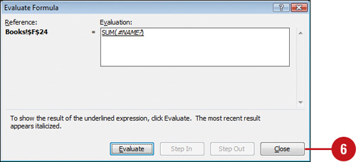
Evaluate a Nested Formula One Step at a Time
![]() Select the cell with the nested formula you want to evaluate. You can only evaluate one cell at a time.
Select the cell with the nested formula you want to evaluate. You can only evaluate one cell at a time.
![]() Click the Formulas tab.
Click the Formulas tab.
![]() Click the Evaluate Formula button.
Click the Evaluate Formula button.
![]() Click Evaluate to examine the value of the underlined reference.
Click Evaluate to examine the value of the underlined reference.
![]() The result of the evaluation appears in italics.
The result of the evaluation appears in italics.
![]() If the underlined part of the formula is a reference to another formula, click Step In to display the other formula in the Evaluation box.
If the underlined part of the formula is a reference to another formula, click Step In to display the other formula in the Evaluation box.
The Step In button is not available for a reference the second time the reference appears in the formula, or if the formula refers to a cell in a separate workbook.
![]() Continue until each part of the formula has been evaluated, and then click Close.
Continue until each part of the formula has been evaluated, and then click Close.
![]() To see the evaluation again, click Restart.
To see the evaluation again, click Restart.
Some parts of formulas that use IF and CHOOSE functions are not evaluated, and #NA is displayed. If a reference is blank, a zero value (0) is displayed.
IMPORTANT Some functions recalculate each time the worksheet changes, and can cause the Evaluate Formula to display different results. These functions include RAND, AREAS, INDEX, OFFSET, CELL, INDIRECT, ROWS, COLUMNS, NOW, TODAY, AND RANDBETWEEN.


Using Constants and Functions in Names
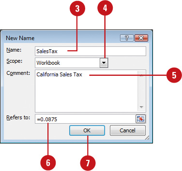
Instead of using a cell to store a constant value or function for use in a formula, you can create a name to store it and then use the name in a formula. If you wanted to calculate sales tax, for example, you could create a name called Sales Tax and assign it a constant value. You can also store text in a name. Instead of typing a long name, such as Environmental Protection Agency, you could create a name called EPA and then use the easy-to-type three letter abbreviation in a formula. When you use EPA in a formula as a text string, Excel replaces it with Environmental Protection Agency. It also works for functions and nested functions.
Use a Constant or Function in a Name
![]() Click the Formulas tab.
Click the Formulas tab.
![]() Click the Define Name button.
Click the Define Name button.
![]() Type a name for the reference.
Type a name for the reference.
![]() Click the Scope list arrow, and then click Workbook or a specific worksheet.
Click the Scope list arrow, and then click Workbook or a specific worksheet.
![]() If you want, type a description of the name.
If you want, type a description of the name.
![]() The current selection appears in the Refers to box.
The current selection appears in the Refers to box.
![]() In the Refers to box, type = (equal sign) followed by the constant, text, or function you want to use.
In the Refers to box, type = (equal sign) followed by the constant, text, or function you want to use.
=.0875, or =“Environmental Protection Agency”
![]() Click OK.
Click OK.