2.4 Dynamic Model of a Mobile System With Constraints
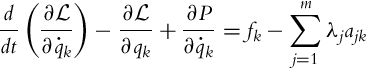
The kinematic model only describes static transformation of some robot velocities (pseudo velocities) to the velocities expressed in global coordinates. However, the dynamic motion model of the mechanical system includes dynamic properties such as system motion caused by external forces and system inertia. Using Lagrange formulation, which is especially suitable to describe mechanical systems [14], the dynamic model reads

where index k describes the general coordinates qk (k = 1, …, n), ![]() defines the Lagrangian (difference between kinetic and potential energy of the system), P is the power dissipation function due to friction and damping in the system, gk are the forces due to gravitation,
defines the Lagrangian (difference between kinetic and potential energy of the system), P is the power dissipation function due to friction and damping in the system, gk are the forces due to gravitation, ![]() are the system disturbances, and fk are the general forces (external influences to the system) related to the general coordinate qk. Eq. (2.46) is valid only for a nonconstrained system, that is, for the system without constraints that has n DOFs and no velocity constraints.
are the system disturbances, and fk are the general forces (external influences to the system) related to the general coordinate qk. Eq. (2.46) is valid only for a nonconstrained system, that is, for the system without constraints that has n DOFs and no velocity constraints.
For systems with motion constraints the dynamic motion equations are given using Lagrange multipliers [15] as follows:
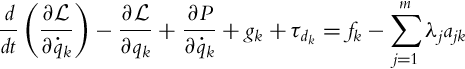
where m is the number of linearly independent motion constraints, λj is the Lagrange multiplier associated with the jth constraint relation, and ajk (j = 1, …, m, k = 1, …, n) are coefficients of the constraints.
The final set of equations consists of n + m differential and algebraic equations (n Lagrange equations and m constraints equations) with n + m unknowns (n general coordinates qk and m Lagrange multipliers λj). Equations are differential in generalized coordinates and algebraic regarding Lagrange multipliers.
A dynamic model (2.47) of some mechanical system with constraints can be expressed in matrix form as follows:
where the meaning of matrices is described in Table 2.1.
Table 2.1
Meaning of matrices in the dynamic model (2.48)
| q | Vector of generalized coordinates (dimension n × 1) |
| M(q) | Positive-definite matrix of masses and inertia (dimension n × n) |
| Vector of Coriolis and centrifugal forces (dimension n × 1) | |
| Vector of friction and dumping forces (dimension n × 1) | |
| G(q) | Vector of forces and torques due to gravity (dimension n × 1) |
| τd | Vector of unknown disturbances including unmodeled dynamics (dimension n × 1) |
| E(q) | Transformation matrix from actuator space to generalized coordinate space (dimension n × r) |
| u | Input vector (dimension r × 1) |
| AT(q) | Matrix of kinematic constraint coefficients (dimension m × n) |
| λ | Vector of constraint forces (Lagrange multipliers) (dimension m × 1) |
2.4.1 State-Space Representation of the Dynamic Model of a Mobile System With Constraints
In the sequel a state-space dynamic model for a system with m kinematic constraints is derived. Then partial linearization of the system state-space description is performed using a nonlinear feedback relation [6] that enables the second-order kinematic model to be obtained.
A dynamic system with m kinematic constraints is described by
where the influence of unknown disturbances and unmodeled dynamics from Eq. (2.48) is left out. The kinematic motion model is given by
The dynamic model (2.49) and kinematic model (2.50) can be joined to a single state-space description. A unified description of nonholonomic and holonomic constraints can be found in [16], where holonomic constraints are expressed in differential (with velocities) form like nonholonomic constraints.
Due to shorter notation the dependence on q is omitted in the following equations (e.g. M(q) or S(q) is written as M or S, respectively). A time derivative of Eq. (2.50) is
Inserting into Eq. (2.49) and expressing generalized coordinates q with pseudo velocities v results in
The presence of Lagrangian multipliers λ due to motion constraints can be eliminated by considering relation AS = 0 and its transform STAT = 0. Multiplying Eq. (2.52) by ST therefore gives a reduced dynamical model:
where Lagrange multipliers λ are eliminated. Introducing ![]() ,
, ![]() , and
, and ![]() gives a more transparent notation,
gives a more transparent notation,
from where a vector of pseudo accelerations ![]() is expressed:
is expressed:
If condition ![]() is true (which in most of realistic examples is) then from Eq. (2.54) the system input can be expressed as
is true (which in most of realistic examples is) then from Eq. (2.54) the system input can be expressed as
By extending the state vector with pseudo velocities x = [qTvT]T and presenting the system in nonlinear form ![]() (expression f(x) contains nonlinear dependence from states) the state-space representation of the system reads
(expression f(x) contains nonlinear dependence from states) the state-space representation of the system reads

where r is the number of inputs in vector u and state vector x has the dimension (2n − m) × 1.
Using the inverse model (2.56) the required system input can be calculated for the desired pseudo accelerations of the system. Applying these inputs to Eq. (2.57) the resulting model becomes

where uz are pseudo accelerations of the system. Relation (2.56) can therefore be used for calculating the required predicted system inputs. These inputs can be used to control the system without feedback (open-loop control) or they are better used as feedforward control in combination with some feedback control.
2.4.2 Kinematic and Dynamic Model of Differential Drive Robot
The differential drive vehicle in Fig. 2.3 has two wheels usually powered by electric motors. Let us assume that the vehicle mass center coincides with its geometric center. The mass of the vehicle without the wheels is mv, and the mass of the wheels is mw. The vehicle moves on the plane and its moment of inertia around the z-axis is Jv (z is in the normal direction to the plane), and the moment of inertia for the wheels is Jw.
In practice usually the mass of the wheels is much smaller than the mass of the casing; therefore a common mass m and inertia J can be used. The vehicle is described by three generalized coordinates q = [x, y, φ] and its input is the torque on the left and the right wheel, τl and τr, respectively (Fig. 2.18).

Kinematic Model and Constraints
The kinematic model (2.2) of the vehicle is

The nonholonomic motion constraint is
which means that the reachable motion directions are columns of the kinematic matrix
and the constraint coefficient matrix is
Dynamic Model
The dynamic model is derived by Lagrange formulation:
where unknown disturbance ![]() from relation (2.47) is omitted. Similarly the forces and the torques due to the gravitation gk are not present because the vehicle drives on the plane where the potential energy is constant (without loss of generality WP = 0 can be assumed).
from relation (2.47) is omitted. Similarly the forces and the torques due to the gravitation gk are not present because the vehicle drives on the plane where the potential energy is constant (without loss of generality WP = 0 can be assumed).
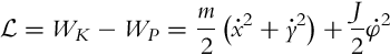
Overall, kinetic energy of the system reads

The potential energy is WP = 0, so the Lagrangian is
Additionally damping and friction at the wheels rotation can be neglected (P = 0). Forces and torques in Eq. (2.61) are

and

According to Lagrange formulation (2.61) the following differential equations are obtained:

where the resultant force on the left and the right wheel is ![]() and r is the wheel radius. The force in the x-axis direction is
and r is the wheel radius. The force in the x-axis direction is ![]() and in the y-axis it is
and in the y-axis it is ![]() . Torque on the vehicle is obtained by
. Torque on the vehicle is obtained by ![]() , where L is the distance among the wheels. Therefore, the final model is
, where L is the distance among the wheels. Therefore, the final model is

The obtained dynamic model written in matrix form is
where matrices are

and the remaining matrices are zero.
The common state-space model (2.57) that includes the kinematic and dynamic model is determined by matrices

and according to Eq. (2.57) the system can be written in the state-space form ![]() , where the state vector is x = [qT, vT]T. The resulting model is
, where the state vector is x = [qT, vT]T. The resulting model is

The inverse system model is obtained by taking into account Eq. (2.56) as

Using the inverse model the required input torques to the wheels can be obtained from the known robot velocities and accelerations. The obtained input torques can be applied in open-loop control or better as a feedforward part in a closed-loop control.
Example 2.9
Derive the kinematic and dynamic model for a vehicle with differential drive in Fig. 2.19. Express the models with the coordinates of the mass center (xc, yc), which are distance d away from the geometric center (x, y).

Solution
Considering the transformation between the geometric and mass center ![]() and
and ![]() and their time derivatives
and their time derivatives ![]() and
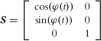
and ![]() and inserting the derivatives to kinematic model (Fig. 2.3), the final kinematic model and kinematic constraint for the mass center are obtained:
and inserting the derivatives to kinematic model (Fig. 2.3), the final kinematic model and kinematic constraint for the mass center are obtained:

The Lagrangian for the mass center is ![]() . Considering relation (2.61) the dynamic model is
. Considering relation (2.61) the dynamic model is
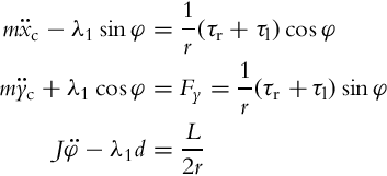
and matrices for the model in matrix form are the following:

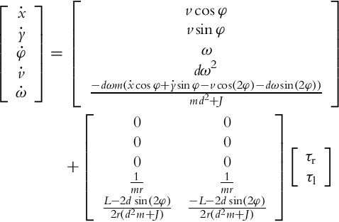
Considering Eq. (2.57) the overall state-space representation of the system reads

Example 2.10
Derive the kinematic and dynamic model for a vehicle in Example 2.9 where the mass center and geometric center are not the same. Express the models using coordinates of the geometric center (x, y), which could be more appropriate in case that the mass center of the vehicle is changing due to a varying load.

Example 2.11
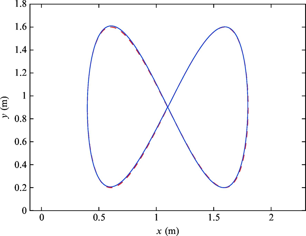
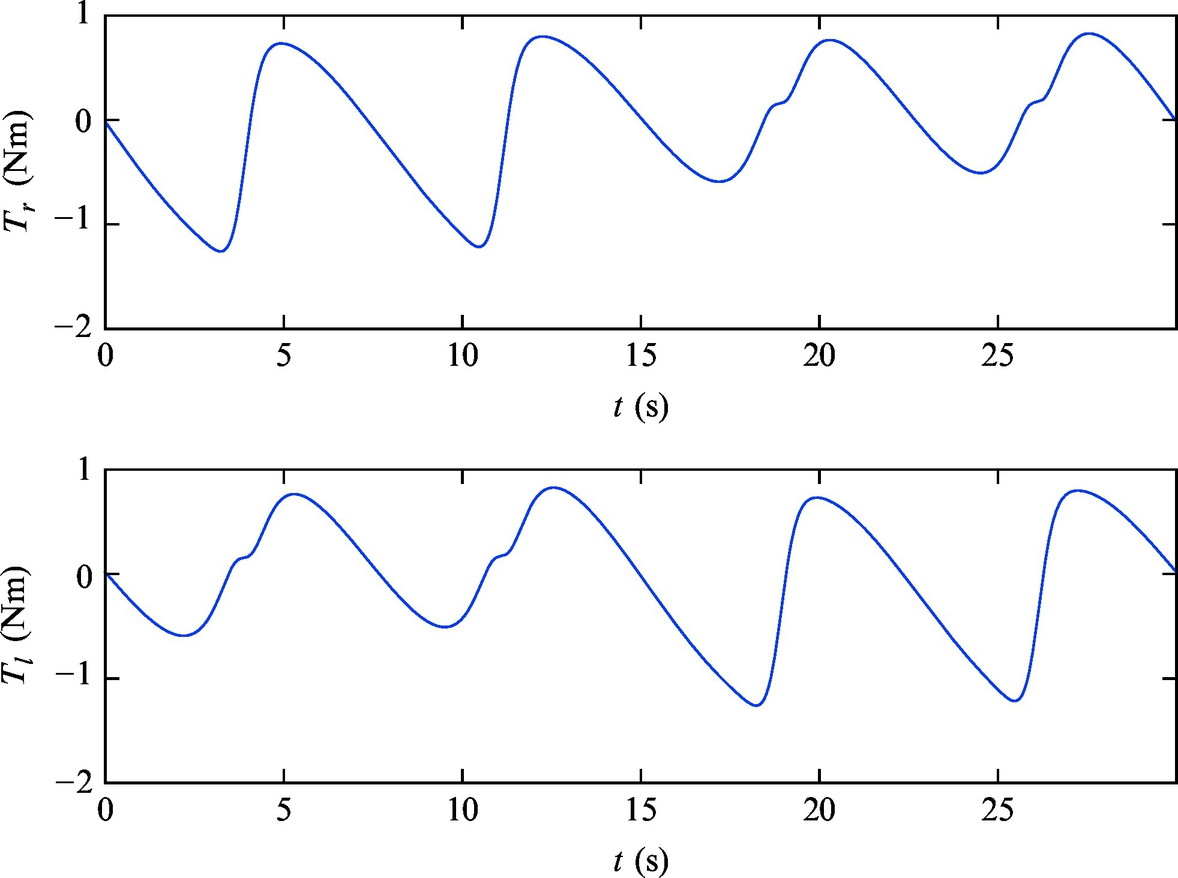
Using Matlab calculate the required torques so that the mobile robot from Example 2.9 will drive along the reference trajectory ![]() ,
, ![]() without using sensors (open-loop control). In the simulation calculate robot torques using the inverse dynamic model, and depict system trajectory. Robot parameters are m = 0.75 kg, J = 0.001 kg m2, L = 0.075 m, r = 0.024 m, and d = 0.01 m.
without using sensors (open-loop control). In the simulation calculate robot torques using the inverse dynamic model, and depict system trajectory. Robot parameters are m = 0.75 kg, J = 0.001 kg m2, L = 0.075 m, r = 0.024 m, and d = 0.01 m.
Solution
The inverse robot model considering relation (2.56) is

From the reference, trajectory reference velocity vr and reference angular velocity ωr and their time derivatives ![]() and
and ![]() are calculated.
are calculated.
Obtained responses using Matlab simulation in Listing 2.3 are shown in Figs. 2.20 and 2.21. 6.88.8