
Plasma Concepts
1.1 Introduction
When a neutral gas is ionized, it behaves as a conductive media. Ionization process is the phenomenon associated with striping electrons from the atoms thus creating the pair of negatively and positively charged particles. Electrical properties of such ionized gas depend on the charged particle density. One of the most important distinctions between the ionized gas and the neutral media is that Coulomb interaction between charged particles determines the dynamic of the gas. Ionized gas is able to conduct the current. This property is of particular interest in the presence of the magnetic field when the interaction of the current and magnetic field leads to electromagnetic body force thus altering its flow dynamics. There are weakly ionized gases and strongly ionized gases. Weekly ionized gas is characterized by a relatively small fraction of charged particles and its behavior can be largely described by neutral gas laws while one needs to invoke electrodynamics to describe appropriately the strongly ionized media. We shall call a physical state of an ionized gas in which the densities of positively and negatively charged particles are approximately equal as a quasi-neutrality state. Plasma is defined as an ionized gas, which satisfies the quasi-neutrality condition.
Development of the plasma physics was always associated with particular applications. Starting from lighting sources, current interrupters, thermonuclear fusion, and plasma accelerators, nowadays plasma applications range from plasma processing, space propulsion, nanotechnology, and plasma medicine.
Prominent physicists contributed to developing the field of the plasma physics and engineering. Irving Langmuir (1881–1957) initiated an active study of the plasma as a new direction of science. The term “plasma” was introduced in 1928 in his article describing the positive column of low-pressure gas discharge. While Langmuir introduced the term plasma, the matter in the plasma state was known to human since much early times. Lighting, northern light, solar wind, and Earth ionosphere are some examples of plasmas. Irving Langmuir received the Nobel Prize in Chemistry, 1932. Mott-Smith indicated in his letter [1] that Langmuir takes the term by analogy between “the blood plasma carries around red and white corpuscles and germs” and the multicomponent ionized gas. The great success in developing the foundation of the plasma science was achieved by Langmuir due to effective collaboration with his famous coworkers Compton, Tonks, Mott-Smith, Jones, Child, and Taylor.
Hannes Alfven (1908–1995) is widely known, as a father of the plasma magnetohydrodynamics. He developed theories regarding the nature of the galactic magnetic field and space plasmas. Prof. Alfven received a Nobel Prize in Physics in 1970 for “fundamental work and discoveries in magnetohydrodynamics.”
Plasma physics, as it is known today, was developed over last 50 years and encompasses many areas ranging from the high-temperature plasmas of thermonuclear fusion to the low-temperature plasma in material processing. The plasma fundamentals and configurations for thermonuclear fusion applications were formulated and developed by Igor Tamm, Andrei Sakharov, Lev Artzimovich, Marshall Rosenbluth, Lyman Spitzer, and many others. Science of the interstellar ionized medium and astrophysical plasmas was by Yakov Zeldovich and Vitaly Ginsburg. Gas discharge plasma physics was introduced by A. von Engel, M. Steenbeck, and then developed by Loeb, Townsend, Thomson, Kaptzov, Granovsky, and Raizer.
In the following as a way of introduction to plasma physics, we will discuss some basic plasma properties. It can be indicative of what kind of plasma is considered by analyzing two main characteristics of plasma behavior in time and space-plasma, i.e. plasma oscillation and Debye length. These two parameters quantitatively describe the plasma and depend on plasma density and temperature.
Let us first focus on understanding of the plasma quasi-neutrality phenomena and its importance. Any perturbation in plasma such as shift of electrons with respect to ions leads to charge separation. The charge separation produces the electric field that works to restore the unperturbed plasma. Let us consider the quasi-neutrality phenomena in the plasma of the high-current vacuum interrupter. As an example, fully ionized plasma is formed with the electron density of about 1022 m−3 and in the volume with radius of about 1 mm. If plasma quasi-neutrality is violated due to charge separation at the characteristic distance of about 1 mm, the electric field of about 1011 V/m will appear. This means that the voltage drop of about 108 V will be set at the distance of about 1 mm. It is clear that such large electric field will work to restore the charge neutrality. However, if relatively small plasma volume is considered, such electric field and potential drop might not be strong enough to affect the particle motion and restore the quasi-neutrality. Thus, quasi-neutrality condition can be violated at the small scale. The characteristics scale where charge separation can exist is called the Debye length.
1.1.1 Debye length
The electrical neutrality or quasi-neutrality is preserved over some characteristic length scale. Let us determine this length scale.
The characteristic length can be obtained from the following argument. The potential energy of the charged particle in the case of full charge separation by distance of about LD is of the order of the particle thermal energy kTe. Maximum possible potential energy due to full separation of charges can be estimated in the planar capacitor case as ![]() Thus one can obtain that
Thus one can obtain that
![]()
where N0 is the charge particle density. From this equality, one can obtain that the characteristic distance of the charge separation is ![]() This distance we shall call the Debye length.
This distance we shall call the Debye length.
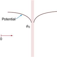
The same expression for the Debye length can be obtained by considering potential shielding in plasmas. We shall examine initially electrically neutral plasma with density N0. To this end it can be supposed that an electric field disturbs the plasma equilibrium state by, for example, immersing the transparent sheet having the negative potential Φ0 with respect to the plasma as shown in Figure 1.1. We will consider one-dimensional plane geometry. As response to the charge perturbation ion and electron distribution will be rearranged to a new state that will correspond to the disturbed electric field. Since ions are heavy particle, their response time is much larger than that of electrons. By taking this into account, we can assume that ions will not be moving on the timescale of interest. This allows us to assume that ion density Ni in the entire plasma region will remain the same as before, i.e., equal N0.
On the other hand, electrons with temperature Te will respond to the repelling electric field and their density will decrease. Electron density can be calculated from the Boltzmann relation as
![]() (1.1)
(1.1)
here φ is the potential. The potential φ distribution in the perturbed region can be calculated using the Poisson equation:
![]() (1.2)
(1.2)
Substituting Eq. (1.1) into Eq. (1.2) will lead to the following:
![]() (1.3)
(1.3)
Assuming that the disturbed energy is small in comparison with the temperature yielding expansion in the Taylor series:
![]() (1.4)
(1.4)
Taking into account only first-order terms in the Taylor series (Eq. (1.4)), the Poisson equation will have the following form:
![]() (1.5)
(1.5)
Using the following denote ![]() the solution of the above equation can be expressed as
the solution of the above equation can be expressed as
![]() (1.6)
(1.6)
Parameter LD is named the Debye length and it is the fundamental characteristics of plasmas. The solution for potential distribution Eq. (1.6) shows that disturbed φ significantly decreased at distance of length LD and demonstrates the screening length over which the plasma neutrality will be preserved. Thus electric field will be shielded at the Debye length scale and plasma will remain quasi-neutral far from the perturbed region.
1.1.2 Plasma oscillation
In this section we will discuss temporal behavior of the plasma. Since plasma is electrically neutral, any violation from quasi-neutrality leads to the formation of a high electric field that restores it. Such electric field appears due to large difference between ion and electron masses. Any electron motion affects the microscale electric field and, as a result, electrons oscillate around ions. Let us describe a simplified model of plasma oscillations assuming uniform cold plasma with density Ne and neglecting the electron thermal motion. When such uniform system will be perturbed, the electrons will be shifted with respect to ions as shown in Figure 1.2.
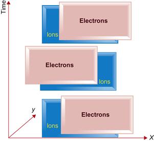
As electrons move, a net positive charge of ions will be left. It is plausible to assume that at the electron timescale ions, will not be moving since their mass is much larger. Due to charge separation, the induced electric field E will act to reduce this charge separation and to accelerate electrons back. Electron will gain kinetic energy and their inertia will cause them passing their original position. As a result, the plasma became again charge separated and an electric field will be formed again in the opposite direction. If there is no damping mechanism (for instance, collisions), these oscillations will continue forever. To calculate the frequency of these oscillations, an electric field can be evaluated using the Gauss theorem that is applied to rectangular region:
![]() (1.7)
(1.7)
where q is the charge in the volume V, s is the surface area, and ε0 is the permittivity:
![]() (1.8)
(1.8)
Thus one can see that the electric field can be calculated as:
![]() (1.9)
(1.9)
The equation of motion for electrons:
![]() (1.10)
(1.10)
After substituting Eq. (1.9) into Eq. (1.10), the following will be obtained:
![]() (1.11)
(1.11)
where me is the electron mass and t is the time. Designate new parameter as

The equation of oscillation can be written as
![]() (1.12)
(1.12)
where ωp is the plasma frequency. This equation has the following solution:
![]() (1.13)
(1.13)
where A1 and A2 are the amplitudes of oscillations which can be determined as constants of integration using the initial condition. It is interesting to note that these oscillations are described by the frequency ωp, which is one of the major characteristics of the plasma. In the absence of collisions and thermal effect, this frequency uniquely determines the oscillation in the plasma. These oscillations are localized and do not propagate. Thermal effect leads to propagation of the oscillation, i.e., generation of the plasma wave or Langmuir wave that will be described in Section 1.2. Collisions can lead to the damping of the oscillation and Langmuir wave propagation that is also subject to a separate analysis described in Section 1.2.
1.1.3 Plasma types
Our daily life involves plasmas in various ways. The spark that jumps between the contacts represents the plasma associated with electrical spark discharge in air, plasma displays have captured the attention of the industry due to the quality of the picture they can produce. Nevertheless, under the ordinary conditions on the Earth, plasma is rather a very rare phenomenon. But in Universe, cold solid bodies are an exception. Most of the matter in the Universe is ionized and thus in the plasma state (about 99%). Plasma in the Universe is produced by various mechanisms. In the stars, the neutral atoms are ionized due to high temperature. Interstellar gases are ionized due to the ultraviolet radiation from the stars.
Plasmas produced in Nature and laboratory plasmas are characterized by a wide range of temperatures and pressures. Using the Debye length and plasma frequency which depend on the electron number density and electron temperature, it is possible to classify plasmas as rarified, dense, classical, and quantum. Figure 1.3 demonstrates the diagram of various objects with their plasma parameters. It spans from high-temperature plasmas in thermonuclear fusion reactors to room-temperature cold plasmas in some biomedical application. Let us consider several examples of the plasmas in controlled thermonuclear fusion, arc discharges, and cold plasmas.
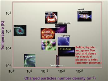
Figure 1.3 Diagram of electron temperature—electron density showing various natural and man-made plasmas.
1.1.3.1 Thermonuclear fusion
High-temperature thermonuclear plasma research was started in 1950 in both the United States and the Soviet Union. The main directions of research were concerned with heating and control of the plasma stability. Since then, for more than half a century, scientists from all over the globe are working on turning the promise of controlled fusion into a practical reality. In fusion reactions that are of interest for energy production, nuclei of light elements combine together to form heavier elements releasing enormous amount of energy. The reactions of greatest interest for fusion energy involve deuterium, a stable isotope of hydrogen whose nucleus contains one proton and one neutron. It should be pointed out that deuterium occurs naturally, making up about 0.015% of all hydrogen.
Steady-state reaction can be supported if power input is balanced by the losses. Power input is supplied externally or from the reaction itself, while power losses are typically due to particle convection to the walls and radiation. Lawson [2] demonstrated that a simple power balance leads to two separate requirements in terms of ion temperature that has to be about 5 keV and a product of the density and confinement time which has to be about 1020 s/m3.
Such temperatures are necessary in order to overcome Coulomb repulsive forces and fuse the deuterium (D=2H) and tritium (T=3H) into helium:
![]()
Recall that the fusion reaction produces much more energy than the nuclear fission. For instance, U235 split releases about 0.8 MeV per nucleon, while D–T fusion into He produces about 3.5 MeV per nucleon.
Lawson’s criterion demonstrates the importance of the plasma confinement. Among various possible confinement approaches, magnetic confinement has been the mainstream approach from the beginning. Several practical magnetic confinement schemes were proposed such as the stellarator (Lyman Spitzer) and tokamak (that was proposed in the former Soviet Union). Tokamak configuration demonstrated the best confinement results. However, it became obvious that further progress will require resources of the international community. An example of this is the Joint European Torus (JET) in Culham, UK, which has been in operation since 1983. In 1991, the JET tokamak achieved the world’s first controlled release of fusion power. Scientists have now designed the next-step device—ITER—that will produce more power than it consumes: for 50 MW of input power, 500 MW of output power will be produced.
1.1.3.2 Vacuum arcs
The vacuum arc is an electrical discharge, which occurs in the vapor ejected from the electrodes. The vapor that forms the conductive path is supplied from small luminous areas on the cathode surface called cathode spots. The concept of the cathode spot unites two physically different regions: the metal surface, which can be heated by the plasma spot to extremely high temperatures, and the near-cathode plasma, which is generated as a result of cathode vaporization and atom ionization. The cathode surface phenomena (electron emission, heating) in the spot area are mutually depended on the phenomena occurring in the spot plasma. Consequently, the combination of these two interacting regions shall be determined by the cathode spot parameters. The near-cathode plasma in the spot is characterized by high particle density, current density, and temperature, which depend on the type of spot and the form of the discharge.
Various theoretical estimates and experiments have determined the following values of near-cathode plasma parameters: heavy particle density N~1024−1026 m−3, degree of ionization is about 0.1–100%, current density J~109–1012 A m−2, electron temperature Te~1–7 eV, ion temperature Ti~0.5–3 eV.
Research on vacuum arc was always closely related to applications. Arc discharges were considered primarily as a lighting source. Over time it was realized that vacuum arc in mercury behaves differently dependent on the electrode polarity. This led to idea that vacuum arc can be used as AC current rectifier. Significant development can be attributed to research at General Electric (Lafferty, Greenwood). Substantial contribution to the physics and application of the mercury vacuum arc was done by Weintraub, Child, Kesaev. Cathode spot is the most complicated phenomenon in the vacuum arc. Ecker, Kesaev, and most recently Beilis developed modern understanding of the complicated cathode spot mechanism.
One of first applications of the vacuum arc was a switching medium in power circuit breakers. The arc is an essential element in the current interruption process. When a pair of current-carrying contacts is separated, current is not interrupted immediately but continues to flow through an arc, which is at once established. One of the earliest definitive works on the subject was done by Sorenson and Mendenhall in 1926, but vacuum switches became available commercially for power system applications only in the beginning of 1960s.
The vacuum arc plasma jet is an excellent source of energetic ions for the deposition of high-quality films. The advantages of this technology are:
good quality films over a wide range of deposition conditions;
retention of alloy composition from the source to the coating.
The applications include the deposition of hard coatings such as TiN and TiAlN, on cutting tools to improve their lifetime and performance, transparent conducting thin films, amorphous semiconducting silicon thin films, and diamond-like carbon film.
In addition, vacuum arcs are used in metal ion accelerators and recently for spacecraft micropropulsion. Microcathode thruster based on the vacuum arc was recently developed. Figure 1.4 illustrates the operation of this thruster in the laboratory conditions.
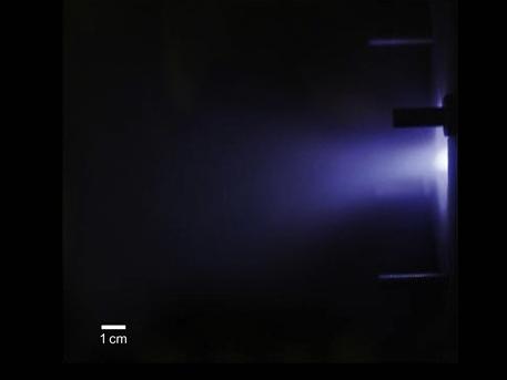
The discharge at the anode is distributed diffusely over the anode surface and this electrode does not suffer erosion. The material used to form the plasma stream is evaporated at microscopic spots on the cathode surface, i.e., on average, a cold, solid surface.
1.1.3.3 Cold plasma
Recent progress in the atmospheric plasmas led to production of the cold plasmas with ion temperatures close to room temperature. This makes these plasmas different from typical low-temperature plasma of a typical electrical discharge. Such plasmas represent very useful tool enabling interaction with biological tissue without thermal damage. Cold plasma technology development resulted in rapid formation of a new field of plasma medicine [3,4]. Typical cold plasma source is shown in Figure 1.5. The plasma source is equipped with pair of high-voltage (HV) electrodes—central electrode (which is isolated from the direct contact with plasma by ceramics) and outer ring electrode as shown schematically in Figure 1.5. Electrodes are connected to a secondary of HV resonant transformer (voltage U up to 10 kV, frequency ~30 kHz). A typical photograph of the plasma jet is shown in Figure 1.5 for U~5 kV and helium feeding corresponding to the flow rate of about υfl=5–10 l/min. The visible plasma jet had a length of approximately 5 cm and was well collimated along the entire length.

Figure 1.5 (A) Schematic view of the plasma gun and (B) typical photograph of plasma jet at U=5 kV and υfl=10 l/min. Source: Reprinted with permission from Ref. [68]. Copyright 2008, American Institute of Physics.
While effects of the electric field on cell was known for a long time [5], cold plasma offers much larger array of possible pathways due to the presence of various chemically active species and charged particles. Cold nonthermal atmospheric plasmas can have tremendous applications in biomedical technology. In particular, plasma treatment can potentially offer a minimum-invasive surgery that allows specific cell removal without influencing the whole tissue. Conventional laser surgery is based on thermal interaction and leads to accidental cell death, i.e., necrosis and may cause permanent tissue damage. In contrast, nonthermal plasma interaction with tissue may allow specific cell removal without necrosis. In particular, these interactions include cell detachment without affecting cell viability, controllable cell death, etc. It can be also used for cosmetic methods of regenerating the reticular architecture of the dermis. The aim of plasma interaction with tissue is not to denaturate the tissue but rather to operate under the threshold of thermal damage and to induce chemically specific response or modification. In particular, presence of the plasma can promote chemical reaction that would have desired effect. Chemical reaction can be promoted by tuning the pressure, gas composition, and energy. Thus the important issues are to find conditions that produce effect on tissue without thermal treatment. Overall plasma treatment offers the advantage that can never be thought of in most advanced laser surgery [6]. For instance, cold plasma demonstrated great promise in cancer therapy [7]. In recent years, cold plasma interaction with tissues becomes very active research topic due to aforementioned potential.
1.1.3.4 Plasma in nature
Atmospheric lightning is probably the most known phenomenon to humans since the early days of humankind. Lightning (shown in Figure 1.6) is an electric discharge, which typically occurs during the thunderstorms. Luminous flashes above thunderstorms have been reported by eyewitnesses for over a century although these flushes were registered only two decades ago [8]. Among them are “red sprites”—optical flashes predominantly in the red located at 50–90 km above ground and associated with giant thunderstorms. Optical observation made with photometers of high spatial resolution revealed that red sprites start as a luminous cloud which then propagates mostly downward developing a highly branched structure as shown schematically in Figure 1.7. Recently upward-propagating stratospheric flashes were identified, named blue jets (BJ) primarily due to blue color. At present, a number of BJ as well as gigantic blue jets (GBJ), propagating into the mesosphere/lower ionosphere, were captured. It appears that the GBJ short-circuit the thundercloud to the ionosphere and thus may have implications for affecting the global electric circuit [9].


1.2 Plasma particle phenomena
1.2.1 Particle collisions
1.2.1.1 Definitions
Plasma particles change their momentum, energy, and states of excitation or charge through particle collisions known as elementary processes. Two types of collisions in plasmas can be distinguished, namely, elastic and nonelastic. Elastic collisions can be broadly defined as events in which the total kinetic energy of particles is conserved and particles retain their original charges. Elastic collisions in which momentum is redistributed between particles involved are described by the following formula:
![]()
Nonelastic collisions are those in which kinetic energy is redistributed between particles and is transferred into some internal mode of one or more colliding particles or into creation of a new particle(s). Nonelastic collisions lead to direct and reverse processes, which include particle excitation and deexcitation, ionization and recombination, charge exchange, dissociation, and charge neutralization. These elementary processes are described by the following formulas:
![]()
Several major ionization pathways can be distinguished in the typical plasma system:
− Direct ionization by electron impact is the ionization of neutrals from the ground state by electrons having high enough energy to cause ionization in a single act. The reverse process is the recombination by which ions capture the free electrons to neutralize the ion into atom. When the ion captured two electrons, the process named three-body recombination and with one electron is the radiative recombination.
![]()
− Stepwise ionization by electron impact is the ionization of previously excited neutral species.
![]()
− Ionization by collisions of heavy atoms in which kinetic energy can lead to ionization process. If chemical energy is important, such process is called associative ionization process.
![]()
− Photoionization process in which ionization is caused by photons interaction with neutral atoms. The reverse process is the photo recombination.
![]()
When a molecular gas is ionized, the reaction can go into excitation of the molecule as well as the molecule can be dissociated. Dissociation is the process when the molecule decayed into separate atoms.
Charge-exchange collisions. Positive ions can collide with atoms and capture a valence electron, resulting in transfer charge from atom to the ion. It can be described as follows:
![]()
Associative ionization is a gas phase chemical reaction in which two atoms/molecules collide and via interaction form an ion. Energy that is released as a result of the chemical reaction is transferred into the electron energy. Ionization occurs if this energy exceeds the ionization potential. One or both of the colliding species may be in the excited state. Such reaction can be written as
![]()
where species A interacts with B to form the ion AB+ and electron.
Penning ionization involves reaction between neutral atoms/molecules. This process is named after Dutch physicist Frans Michel Penning (effect reported in 1927) [10]. The term penning ionization refers to the interaction between an excited-state atom/molecule A and a target atom/molecule B and results in formation of an ion B, electron, and neutral gas atom/molecule A, i.e.,
![]()
Penning ionization occurs when the target atom/molecule B has an ionization potential lower than the internal energy of the excited-state atom/molecule A*. As an example, helium has excited states at very higher energy just below ionization potential, such as energy levels of 19.82 eV for the 23S state and 20.6 eV for 21S state. Such energetic levels are higher than the ionization potential for some gaseous and metal atoms. For instance, nitrogen has ionization potential of 14.5 eV, hydrogen of about 13.5 eV, and titanium of about 6.8 eV.
Coulomb collisions are elastic collisions between charge particles, representing electron–electron, electron–ion, and ion–ion collisions.
A superelastics collision is a process when the internal energy is transferred into the kinetic energy of an emitted particle. An example of this is the Auger effect in which energetic electrons are emitted from an excited atom after a series of internal relaxation events. Deexcitation of metastable atoms and molecules with simultaneous release of an electron is the surface scattering process. The probability for electron release by such process is characterized by the overall secondary electron emission (SEE) coefficient γe, which is the ratio of emitted electrons to number of metastable atom/molecules deexcitation at the surface. γe is about 10−4−10−2 dependent on the atom/surface pair [11–13]. The Auger effect is the basis of the surface-sensitive electron spectroscopy.
1.2.1.2 Cross section: mean free path
The collision probability of each elementary process mentioned above is characterized by particle density and a parameter named cross section. Let us define this parameter in case of elastic collisions considering a single test particle moving through a cloud with a density na of particles at rest (as shown in Figure 1.8) and having only elastic encounters with target particles.
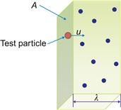
The number of target particles in the volume V is naV and the cross section σ of the target particle is defined as σ=(π/4)d2p, where dp is the diameter of particle. Let us introduce the mean free path for collisions which is the average distance between consecutive collision events as
![]() (1.14)
(1.14)
The frequency of collisions with target particles can be defined as
![]() (1.15)
(1.15)
where u is the test particle velocity.
Let us introduce the collisional mean free path in detail. To that end we consider a simple gas consisting hard-sphere particle. The distance along the line joining the center of any two particles is equal to d (Figure 1.9).

Consider a single test particle z moving in randomly distributed particles at rest as shown in Figure 1.10A. It is assumed an oversimplified situation in which the test particle z moves at a uniform speed equal to the mean molecular speed 〈C〉 and all the other molecules are standing still.

Figure 1.10 (A) Path of molecule z among stationary molecules: actual path and (B) path of molecule z among stationary molecules: imaginary straightened path.
Along the molecule path (Figure 1.10B), the volume trace by the sphere of influence per unit time is πd2〈C〉. For a density of fixed particles, na, the number of particle centers lying within cylinder volume is πd2〈C〉na. Since each of these centers corresponds to a collision, this product must also represent the number Σ of collisions per unit time for test molecule z, i.e.,
![]() (1.16)
(1.16)
In essence, parameter Σ characterizes the collision frequency. The distance travel in time between the collisions characterizes the mean free path λ of the molecule with average velocity 〈C〉 as
![]() (1.17)
(1.17)
More complicated analysis based on the particle kinetics produces very similar results with just a factor ![]() in denominator (1.17):
in denominator (1.17):
![]() (1.18)
(1.18)
The factor ![]() in the denominator arises from the fact that the correct speed to use for the evaluation of Σ in Eq. (1.17) is really the mean relative speed of the molecules, and this can be shown to be
in the denominator arises from the fact that the correct speed to use for the evaluation of Σ in Eq. (1.17) is really the mean relative speed of the molecules, and this can be shown to be ![]() Equation (1.18) can also be written in terms of the mass density ρ=mn, where m is the mass of the assumedly identical molecules. This gives
Equation (1.18) can also be written in terms of the mass density ρ=mn, where m is the mass of the assumedly identical molecules. This gives
![]() (1.19)
(1.19)
Thus for a given value of ρ, the mean free path for the rigid-sphere model is independent of temperature and depends only on the gas density, mass, and diameter of the molecules.
In case of assembly of test particles, the flux density of the particles can be defined as Γ=nu, where n is the particle density (see Figure 1.8). Let us assume that collisions remove particles from the beam. The change of the particle density can be calculated as follows:
![]() (1.20)
(1.20)
and the reduction of the particle flux can be calculated as
![]() (1.21)
(1.21)
Integration of Eq. (1.21) will give the flux dependence on distance x as the following:
![]() (1.22)
(1.22)
After a collision, the test particle scattered by an angle θ of scattered particle trajectory with respect to its incident direction as shown in Figure 1.11. This kind of collisions is characterized by another parameter defined as differential cross section σ(θ). Impact parameter (b, see Figs. 1.11, 1.12) is the perpendicular distance from the original center of a scattering particle to the original line of motion of a particle being scattered.
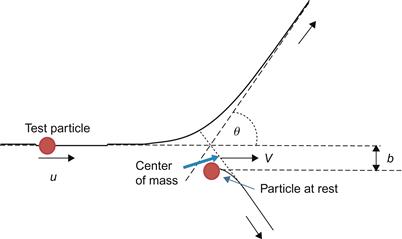
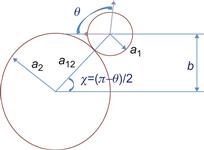
Figure 1.12 Schematics of the hard-sphere collision. a1, a2 are radii of the spheres and a12 is the distance between centers of the colliding spheres.
The probability of the particle emerging into the solid angle is dΩ=sin θ dθ dφ. Integrating over the full solid angle yields the so-named total cross section for a particular collision in the form
![]() (1.23)
(1.23)
For many practical applications, it is important to consider interactions that lead to scatter by θ=90° or more as shown in Figure 1.12. The elastic collision with θ=90° occurs on χ=45°. Thus the cross section in this case is equal to cross section for scattering with angle larger than ![]() The collision cross in the hard-sphere model is
The collision cross in the hard-sphere model is ![]() One can see that 90° is smaller than that of the hard-sphere model by factor of 2.
One can see that 90° is smaller than that of the hard-sphere model by factor of 2.
1.2.1.3 Charge-exchange cross section
Both resonant and nonresonant charge-exchange collisions can take place. Resonant charge exchange occurs between the same atoms, while nonresonant occurs between different atoms. Consider reaction
![]()
Electron transfer from B to A+ occurs in two steps: first, release from B and then capture by A+. By calculating the potential energy of electron in the electrostatic field of A+ and B+ and considering kinetic energy of electron, one can calculate the distance between A and B leading to electron transfer. For the ground state, resonant charge exchange cross section (i.e., A=B) can be estimated as:
![]() (1.24)
(1.24)
where e is the electron charge, ε0 is the permittivity of vacuum, and Ei is the ionization potential. Detailed theoretical analysis and experiment show that cross section for charge exchange has weak dependence on the kinetic energy. While most of data on charge-exchange cross section are obtained experimentally, there are several simplified theories developed.
Sakabe and Izawa [14] calculated cross section for charge-exchange collisions by solving the time-dependent Shrodinger equation. The cross sections of resonant charge transfer between atoms and positive ions for all nontransition elements have been calculated by the impact parameter and close-coupling methods. The calculated results are in good agreement with the experimental results for the elements for which data are available. Figure 1.13 shows the calculation result and the experimental data on the cross section of helium atoms as a function of impact velocity. The calculated results are in good agreement with the experimental results, in particular in the low-velocity range less than 108 cm/s.

Figure 1.13 Cross section—impact–velocity curve for resonant charge transfer of a helium atom. Experimental data are given by symbols and thin lines [14]. A thick dashed line corresponds to calculation result. Source: Reprinted with permission from Ref. [14]. Copyright 1992 by the American Physical Society.
1.2.1.4 Coulomb collision cross section
Let us consider collisions of two particles with charges q1 and q2. This type of interactions occurs between electron–electron, ion–electron, and ion–ion. Particles interact with one another via electrostatic potential:
![]() (1.25)
(1.25)
Coulomb forces are long-range interaction as it depends inversely on distance r2. However, potentials are screened in plasma at the scale of about Debye length LD. Thus the maximum impact parameter can be taken equal to the Debye length since the Coulomb electric field force decays exponentially at the distances larger than LD. In other words, the maximum distance for interactions is bmax~LD. Yet, a collision cross section based on the Debye length, i.e., ![]() is still very large. Taking into account that the electric field is partially screened in the Debye sphere, a collision cross section based on the Debye length includes scattering over very small angles that does not affect significantly transport coefficients. Thus we will limit our consideration of the scattering process by only scattering over large angles, e.g., >90°.
is still very large. Taking into account that the electric field is partially screened in the Debye sphere, a collision cross section based on the Debye length includes scattering over very small angles that does not affect significantly transport coefficients. Thus we will limit our consideration of the scattering process by only scattering over large angles, e.g., >90°.
Scattering to large angles can be due to a single collision scattering over a large angle or due to cumulative effect of many small-angle collisions. In plasmas, because of the long-range nature of the electrostatic interaction, much frequent small-angle collisions led to larger effect than the fewer large angle events. In order to evaluate this effect, one needs to consider the cumulative effect of many scattering of electron by many ions with different values of impact parameter b (Figure 1.12).
Consider electron having initial velocity v that undergoes many small-angle scattering collisions. Each collision event will lead to small increment in electron velocity Δv in all directions. Recall that electron energy is nearly conserved in collision since electron is a light particle that is scattered off a heavy ion, while electron losses its momentum. Thus there is a reduction of the electron velocity in the original direction. The average velocity reduction can be estimated as
![]() (1.26)
(1.26)
where n is the ion density, Z is the ion charge, and ln Λ=ln(bmax/bmin) is called Coulomb logarithm. From this equation, one can define the electron–ion collisional frequency for loss of electron momentum as
![]() (1.27)
(1.27)
To estimate the minimum impact parameter bmin, we need to point out that when the Coulomb potential energy becomes as large as the electron thermal energy, the scattering angle becomes the largest.
Thus bmin can be estimated from the condition that the Coulomb energy is equal to the thermal energy:
![]() (1.28)
(1.28)
The Coulomb logarithm represents the sum of all scattering angles by Coulomb collisions within the Debye sphere. Detailed analysis leads to the following expression for the Coulomb logarithm (if Ti(me/mi)<Te<10Z2 eV [15]):
![]() (1.29)
(1.29)
where Te is in eV and ne is in cm3. In plasma of interest is 5–10 eV. ln Λ is about 17 in the case of fusion plasma and about 10 in the case of arc discharge plasmas.
The total cross section for electron scattering on ions can thus be calculated using relationship between the collision frequency and cross section:
![]() (1.30)
(1.30)
1.2.1.5 Ionization cross section
In general, the quantum mechanical analysis should be employed to describe the cross section of atom ionization. However, some qualitative analysis with reasonable quantitative results was performed using classical approach in physics. In this case, the ionization process was considered as interaction of impact electron with a valence electron of a neutral atom. It was assumed that the atom was ionized if the transferred energy to the valence electron exceeds the ionization potential Ei. This is the basis of the model that was developed by Thomson back in 1912 [16]. According to the Thomson’s model, the ionization takes place if transferred energy is larger than the ionization potential, i.e., E>Ei. After integration over electron energies that is larger than Ei, the following expression for the ionization cross section was obtained [14]:
![]() (1.31)
(1.31)
At very high energies, Thomson model predicts that ionization cross section fall as ~1/E. The cross section has its maximum at E=2Ei. Thus the maximal cross section is
![]() (1.32)
(1.32)
The dependence of the ionization cross section on the electron energy for different atoms is shown in Figure 1.14.

Figure 1.14 Calculated cross section according to the Thomson model (Eq. 1.31).
It should be pointed out that the electron temperature is typically in the order of few electron volts which is smaller than the ionization potential for most atoms of interest. However, the high-energy electrons from the tail of Maxwell distribution play a very important role in the ionization process. In order to obtain the collisional cross section in the case of electron energy distribution, one have to integrate over the velocity distribution:
![]() (1.33)
(1.33)
where ki(T) is the ionization coefficient.
If Maxwellian distribution function can be assumed, we will arrive at the following expression:
![]() (1.34)
(1.34)
In order to calculate the cross section of atom ionization σ(v), one can use the Thomson formula near E=mv2/2~Ei:
![]() (1.35)
(1.35)
where ![]()
With this assumption, the above expression for ionization coefficient becomes the following simple form:
![]() (1.36)
(1.36)
Below the ionization cross sections for electron impact with different materials are demonstrated. An example of total cross section for electron scattering on nitrogen molecules is shown in Figure 1.15 and ionization collision cross section for several gases [18] is shown in Figure 1.16A and B. One can see that total scattering cross section can have several maxima. Peak in ionization cross section is clearly recognizable in both cases.

Figure 1.15 Total scattering cross section of molecular nitrogen (e+N2). Source: Adapted from Ref. [17].

Figure 1.16 (A) Total cross sections for the ionization of atomic xenon. (B) Total cross sections for the ionization of atomic helium. Note: To convert cross sections in ![]() units to 1016 cm−3 cross sections in
units to 1016 cm−3 cross sections in ![]() should be divided by 1.13673. Source: Reprinted with permission from Ref. [18]. Copyright 1966 by the American Physical Society.
should be divided by 1.13673. Source: Reprinted with permission from Ref. [18]. Copyright 1966 by the American Physical Society.
1.2.1.6 Plasma equilibrium
One particular thermodynamic state of the plasma is widely used to describe plasma chemical composition, so called plasma equilibrium. Let us first define the degree of ionization in the plasma. Consider plasma consisting of electrons, ions, and atoms. In the case of a low-ionized plasma, i.e., ne![]() na, the ionization degree is defined as
na, the ionization degree is defined as
![]() (1.37)
(1.37)
In the thermodynamic equilibrium, there are two reactions: direct reaction leading to ionization and a back reaction leading to recombination. In the case considered, the direct reaction is the electron impact ionization and back reaction is the recombination involving three particles. In other words, the stochiometric equation will have the form:
![]()
with the rate of ionization being ki·na·ne and the rate of recombination being kr·ni·![]() where ki and kr are the ionization and recombination coefficient, respectively. We shall define the ionization equilibrium as a state in which ionization and recombination rates are equal.
where ki and kr are the ionization and recombination coefficient, respectively. We shall define the ionization equilibrium as a state in which ionization and recombination rates are equal.
The equilibrium constant K(T) can be defined as follows:
![]() (1.38)
(1.38)
This equation can be solved for the electron density provided that the equilibrium constant dependent on temperature is known as a function of the pressure in the system. If equation of state for the plasma can be specified, this equation can be used to calculate the electron density as a function of the temperature.
Degree of ionization can also be determined from the thermodynamic equilibrium of plasma. We shall illustrate this below. This relationship that can be used to determine the plasma composition in equilibrium is called the Saha equation.
Let us derive the Saha equation from the statistical mechanics. We assume that plasma is in thermodynamic equilibrium, so that we can use a single temperature for all plasma components. The approach that will be used is quasi-classical taking into account statistical weights and quantum phase space. While being an approximation, this approach gives physically illustrative picture of the phenomena.
According to the statistical mechanics, the probability of a particle to be at the energy level ε is determined by the Boltzmann relation:
![]() (1.39)
(1.39)
where T is the plasma temperature.
The number of particles can be calculated by multiplying the probability and number of states. The number of states assuming that particles do not have internal degrees of freedom is equivalent to the number of cells in the phase space h3, where h is the Planck’s constant. The volume in the momentum space for electrons having momentum between p and p+dp equals:
![]() (1.40)
(1.40)
Thus, the number of electrons in the volume V can be calculated as
![]() (1.41)
(1.41)
where ge is the electron degeneracy.
We are considering the equilibrium state of electrons and neutrals and as such let us consider zero energy level corresponds to electrons in atom. It follows that free electron will have the energy
![]() (1.42)
(1.42)
where Ei is the ionization potential. The total number of electrons can then be calculated by integrating over the entire spectrum:
![]() (1.43)
(1.43)
After integration one can find that the electron density has the following expression:
![]() (1.44)
(1.44)
Such quasi-classical approach cannot lead to the complete expression without considering additional assumptions. First of all, recall that in the integral (1.43) it was taken into account the number of electrons per a single atom. In order to calculate the full number of electrons, we have to multiply Ne by number of atoms in one quantum state, i.e., Na/ga. The resulting expression for the number of electrons is thus
![]() (1.45)
(1.45)
Secondly, equilibrium state consists of electrons, neutrals, and ions. Thus, ionization balance must account for ions as well. This can be done by assuming that the volume corresponds to an ion in a given quantum state, i.e.,
![]() (1.46)
(1.46)
By supplementing this expression into Eq. (1.45), we arrive at the final expression for the Saha equation:
![]() (1.47)
(1.47)
Equation (1.47) describes plasma that consists of electrons, atoms, and ions of a single type. However, it can also be used to calculate the composition of gas mixture. Let us demonstrate this on the following example.
Let us start with equations for equilibrium for each individual species. In the case considered, these equations can be written as
![]() (1.48)
(1.48)
![]() (1.49)
(1.49)
where nHei is the density of helium ions and nCi is the density of carbon ions.
Arc plasma consists of the electrons, neutrals C and He, and ions C+ and He+. Thus, we have five unknown densities. In order to calculate an equilibrium composition, we can invoke two additional equations. One is the plasma quasi-neutrality:
![]() (1.50)
(1.50)
Second equation is the equation for atom conservation, i.e., the ratio of total density of atoms and ions of helium to the total density of atoms and ions of carbon:
![]() (1.51)
(1.51)
Finally, the total pressure is equal to the sum of partial pressures of all species.
Plasma composition calculation using Saha equilibrium is shown in Figure 1.17.

One can see that significant ionization starts at temperatures exceeding 12,000 K and it is dominated by ionization of carbon. Ionization of helium atoms starts at about 20,000.
1.3 Waves and instabilities in plasmas
1.3.1 Electromagnetic phenomena in plasma
1.3.1.1 Conservation law for electric charge and current: electromagnetic waves
Each charged particle in plasma has an electric charge. Electron has charge of about 1.6×10⁻¹⁹ C and ion charge being either single or multiple electron charges. While typically ions have a positive charge, negatively charged ions can be created due to electron attachment to atom or molecule. Good example is the oxygen that has very large cross section for electron attachment.
The electrostatic force Fij is determined by the interaction of charges qi and qj with distance rij between the charges in form:
![]() (1.52)
(1.52)
Charge is the additive property, i.e., the total charge in a volume can be expressed as a sum of number particles of type Ni with charges qi:
![]() (1.53)
(1.53)
where qi is the charge of a single particles.
Density of charges per unit volume:
![]() (1.54)
(1.54)
Considering uniform charge distribution in the volume V, current density can be defined as
![]() (1.55)
(1.55)
where v is the average velocity of charges. When charges are distributed nonuniformly in the volume, the total charge can be calculated by integrating over the considered volume:
![]() (1.56)
(1.56)
By employing the Gauss theorem:
![]() (1.57)
(1.57)
one can arrive at the following equation which is the conservation of charges:
![]() (1.58)
(1.58)
Electric and magnetic fields in the plasma must satisfy the Maxwell equations. These equations were proposed by James Maxwell to describe electromagnetic wave propagation in a media:
![]() (1.59)
(1.59)
![]() (1.60)
(1.60)
![]() (1.61)
(1.61)
![]() (1.62)
(1.62)
Introducing the electric potential, one can define the electric field as E=−∇φ, as a result the last equation will have the following form:
![]() (1.63)
(1.63)
Equation (1.63) is called the Poisson equation. If ne=ni, i.e., quasi-neutrality is fulfilled, the Poisson equation will reduce to Δφ=0, which is equivalent to assuming the vacuum electric field. Note that the Poisson equation in reduced form can be used to calculate potential distribution only if plasma is uniform and in the absence of a magnetic field. In a general case, potential distribution in plasma can be calculated invoking the generalized Ohm’s law as will be described in Chapter 4.
1.3.1.2 Electromagnetic wave propagation
Waves can transport energy to and from a media. In order to describe the wave propagation, we will use Eqs (1.59) and (1.60). Two limited cases can be considered, namely, a media with high conductivity and a media with low conductivity.
1.3.1.2.1 Propagation in a media with high conductivity (i.e., metal)
In this case it can be safely assumed that
![]() (1.64)
(1.64)
For a high conductive media, the set of Maxwell equations can be written as follows:
![]() (1.65)
(1.65)
![]() (1.66)
(1.66)
![]() (1.67)
(1.67)
![]() (1.68)
(1.68)
The Ohm’s law reads
![]() (1.69)
(1.69)
where σ is the conductivity of metal. Employing the wave in the form of E,H~exp(j[kr−ωt]), where j is the imaginary unit, k is called the propagation constant, and ω is the frequency of the wave. Substituting the waveform into Eqs (1.65) and (1.66) leads to
![]()
where ![]() is the amplitude of the magnetic field. Apply ∇× operator to both sides of this equation:
is the amplitude of the magnetic field. Apply ∇× operator to both sides of this equation:
![]()
Using operator properties and Eq. (1.66), this equation can be rewritten as
![]()
Taking into account Eq. (1.68) i.e., ∇·E=0, this equation can be reduced to the following equations for electric fields:
![]() (1.70)
(1.70)
The same approach can be applied to the magnetic field:
![]() (1.71)
(1.71)
where ![]()
Considering the problem of wave propagation in one-dimensional approximation, the amplitude of the electric and magnetic fields can be written as
![]() (1.72)
(1.72)
![]()
where E0 and B0 are the amplitudes of the electric and magnetic fields at the boundary as shown in Figure 1.18. Let us analyze the parameter γ:
![]() (1.73)
(1.73)

The real part of the parameter γ is equal to
![]()
Thus the expression for the electric field amplitude has the following form:
![]() (1.74)
(1.74)
One can see that the amplitude E=E0 exp(−αx) of the electric field decreases with distance. The parameter 1/α is the characteristic length, which is called a skin layer. The skin layer thickness can thus be calculated as
 (1.75)
1.3.1.2.2 Propagation in a media with low conductivity (i.e. dielectric)
In this case one can assume that J![]() ε0(∂E/∂t), i.e., in this case only a displacement current can be considered. Using the same approach as in the case of a wave propagation in the conductor, we arrive at the following equations:
ε0(∂E/∂t), i.e., in this case only a displacement current can be considered. Using the same approach as in the case of a wave propagation in the conductor, we arrive at the following equations:
![]() (1.76)
(1.76)
![]() (1.77)
(1.77)
where ![]() Thus in this case the parameter γ has only an imaginary part. This means that there is no damping of the wave. This is shown schematically in Figure 1.19.
Thus in this case the parameter γ has only an imaginary part. This means that there is no damping of the wave. This is shown schematically in Figure 1.19.

1.3.2 Waves in plasma
Any periodic motion of plasma can be decomposed into a superposition of sinusoidal oscillations with frequency ω and wavelength λ. In the following, we will consider that any quantities (density n, velocity v, electric field E) have sinusoidal waveform. Thus, the plasma density is represented as
![]() (1.78)
(1.78)
where ![]() is the density amplitude, k·r=kxx+kyy+kzz is the vector of wave propagation. In a simple one-dimensional case is
is the density amplitude, k·r=kxx+kyy+kzz is the vector of wave propagation. In a simple one-dimensional case is ![]() Recall that the measurable quantity is in the real part:
Recall that the measurable quantity is in the real part:
![]() (1.79)
(1.79)
A point of constant phase of the wave moves so that d/dt(kxx−ωt)=0 or in other words
![]() (1.80)
(1.80)
where vφ is the phase velocity. Similarly electric field can be expressed:
![]() (1.81)
(1.81)
where δ is the phase shift with respect to the density oscillations as given in Eq. (1.79).
Note: Phase velocity can exceed the speed of light! However, this does not violate the theory of relativity because wave of constant amplitude does not carry any information. Information is carried only when wave is modulated. The modulation is traveled with velocity vg, which is the group velocity of the wave.
Let us define the group velocity. For this reason we will consider the two added “beating” waves with the following conditions:
![]() (1.82)
(1.82)
![]() (1.83)
(1.83)
Using the following new denotation:
![]()
![]()
Summation of two electric fields will give the following:
![]() (1.84)
(1.84)
![]() (1.85)
(1.85)
It follows that the envelope of such wave is given by cos(Δkx−Δωt). Equation (1.85) can be interpreted as a simple wave with modulated amplitude 2 cos(Δkx−Δωt). In other words, the amplitude of the wave is itself a wave, and the phase velocity of this modulation wave is Δω/Δk. The propagation of information or energy in a wave occurs as a change in the wave. The simplest example is transition from the wave being absent to being present, which propagates at the speed of the leading edge of a wave train. In a more general sense, some modulation of the frequency and/or amplitude of a wave is required in order to convey information, and it is this modulation that represents the signal content. Thus the speed of information propagation can be described as Δω/Δk. This is the phase velocity of the wave amplitude, but since each amplitude wave may contain a group of internal waves, this speed is called the group velocity:
![]()
It should be pointed out that in accordance with theory of relativity, the group velocity vg is always smaller than the speed of light, i.e., vg≤c.
1.3.3 Plasma oscillations
Any disturbance of an electric field in the plasma can displace the electrons from the uniform background of ions. As a result, an internal electric field will appear to restore the neutrality of plasma by pulling electrons back. Because of negligible inertia, electrons are overshooting and as a result will oscillate around their equilibrium position. On the timescale considered, ions are not responded to the oscillations. Such oscillations will occur at the so-called plasma frequency ωp.
Consider wave propagation in such plasma under the following conditions: no magnetic field; all particles are cold (i.e., kBT=0); ions are not moving; plasma is infinite.
Under these conditions, a 1D equation for electron motion and continuity can be written as follows:
![]() (1.86)
(1.86)
![]() (1.87)
(1.87)
Poisson’s equation reads
![]() (1.88)
(1.88)
This system describes plasma state including its temporal evolution. Equations (1.86)–(1.88) will be employed in order to analyze the electron oscillations in plasma. To this end, the system of equations (1.86)–(1.88) will be linearized assuming that the amplitude of oscillation is small and using the standard approach of small perturbation, the plasma parameters from their respected equilibrium state:
![]()
![]() (1.89)
(1.89)
![]()
where subscript “0” corresponds to the equilibrium part and subscript “1” corresponds to the perturbation part. In the framework of oscillations with small amplitude, the following condition take place:
![]()
![]() (1.90)
(1.90)
![]()
In addition, we consider uniform quasi-neutral plasma is at rest:
![]() (1.91)
(1.91)
![]() (1.92)
(1.92)
Taking into account the above conditions and assumption, and neglecting the second-order terms we arrive at the following simplified system of equations:
![]() (1.93)
(1.93)
![]() (1.94)
(1.94)
or after implementing the assumption that plasma is uniform we arrive at the following:
![]() (1.95)
(1.95)
The condition that all oscillating properties behave sinusoidal is considered, i.e.,
![]()
![]() (1.96)
(1.96)
![]()
Let us substitute these expressions into Eqs (1.93) and (1.95). After differentiating these equations, the system of equations of interest (Eqs (1.93) and (1.95)) is reduced to the following algebraic equations:
![]()
![]() (1.97)
(1.97)
![]()
The system of equation (1.97) can be solved for frequency ω and result in
![]() (1.98)
(1.98)
For instance, in the case of a density of about 1018 m−3, plasma frequency (ω/2π) is about 9 GHz. It should be pointed out that group velocity for plasma oscillations, i.e., Vg=∂ω/∂k=0 and therefore disturbance associated with plasma oscillation does not propagate, i.e., localized. While plasma oscillations are standing, the thermal motion of electrons can cause plasma wave to propagate. In the next section, we will consider electron plasma wave, which is developed due to electron thermal motion.
1.3.4 Electron plasma wave
Consider the case that electrons are streaming from the oscillating region due to presence of density gradient and their thermal motion. Such electron flux carries information about oscillation from the oscillating localized area thus creating the wave. This wave is called a plasma wave.
In order to account for the effect of wave formation, one needs to consider an additional term in the electron momentum (1.93), i.e., the electron pressure gradient ∇Pe. For our analysis, we will use the adiabatic index γ=3 in the one-dimensional case:
![]() (1.99)
(1.99)
Now the equation of motion for electrons will have the following form:
![]() (1.100)
(1.100)
After substitution of the sinusoid waveform, we arrive at the following:
![]() (1.101)
(1.101)
If we express both perturbed density n1 and electric field E1 as a function of perturbed velocity V1, we arrive at the following relation:
![]() (1.102)
(1.102)
This equation can be modified and solved for the frequency leading to dispersion relation:
![]() (1.103)
(1.103)
where ![]()
It follows from this dispersion relation that frequency depends on the wave number. Differentiating the last expression leads to
![]()
From here one can find that:
![]() (1.104)
(1.104)
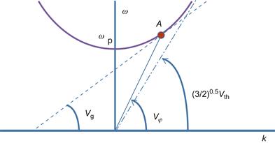
Diagram of the plasma wave (correspondent to Eq. (1.103)) is shown in Figure 1.20. At any point on the dispersion curve, it is possible to define the group velocity and the phase velocity. From the diagram, one can note that in the case of large k (small wavelength λ), plasma wave travels at Vth.
It should be pointed out that existence of plasma waves was known since the time of Langmuir. Sometimes these waves are called Langmuir waves. Complete theory of these waves was developed by Bohm and Gross [19].
1.3.5 Sound waves in plasma
Sound waves propagate in gas due to collisions. Sound waves in plasmas can propagate even in absence of collisions by electron–ion coupling via the electric field. Since heavy particles are involved, such plasma oscillations will be in a low-frequency range. Let us illustrate these oscillations considering plasma quasi-neutrality condition, i.e., ne=ni.
Starting with ion momentum equation:
![]() (1.105)
(1.105)
Linearization of this equation leads to
![]() (1.106)
(1.106)
Boltzmann relation for electrons is employed:
![]() (1.107)
(1.107)
Assuming that perturbations are small, one can use Taylor expansion:
![]() (1.108)
(1.108)
From the linearized ion continuity (Eq. (1.97)), it can be found:
![]() (1.109)
(1.109)
Substituting expression for the fluctuating density n1 into the ion momentum (1.106), the following relationship is obtained:
![]() (1.110)
(1.110)
Solving this equation for the frequency, one can arrive at the following dispersion relation:
![]() (1.111)
(1.111)
As it is seen from Eq. (1.111), the considered wave has the linear dispersion relation and the same phase and group velocity, i.e.,
![]() (1.112)
(1.112)
where Vs is the acoustic velocity. It is interesting to note that ion wave still exist even if ion temperature Ti=0. This can be understood as follows. In ion oscillations, electrons are not fixed; electrons are pulled along with ions shielding the electric field that can arise from ion motion. However, shielding of the electric field is not perfect and an electric field about kTe/e can leak due to electron thermal motion as it was discussed above. As an ordinary sound wave, ions form regions of rarefaction and compression as shown schematically in Figure 1.21. The compression region expands into the rarefaction region due to ion thermal motion (this is the second term in Eq. (1.112)) and electric field due to electrons (first term in Eq. (1.112)). The sound speed depends on electron temperature since electric field is proportional to it and ion mass since ion inertia depends on it.

In other words, ion wave propagates due to two reasons: ion thermal motion that makes it similar to the sound wave in neutral gas and presence of the electric field in a quasi-neutral plasma that couples ions and electrons motion.
Note that we used a quasi-neutrality condition to derive the ion wave. If quasi-neutrality condition is relaxed and thus Poisson equation is used to calculate the electric field, one can obtain the modified dispersion relation:
 (1.113)
One can see that this equation is the same as Eq. (1.112) except for the factor ![]() Since Debye length is small, the quasi-neutral approximation is usually valid except for shortest wavelength (large k). The generalized dispersion relation is shown in Figure 1.22.
Since Debye length is small, the quasi-neutral approximation is usually valid except for shortest wavelength (large k). The generalized dispersion relation is shown in Figure 1.22.

If oscillations are short wavelength, i.e., (kλD)2![]() 1, one can find (from Eq. (1.113)):
1, one can find (from Eq. (1.113)):
![]() (1.114)
(1.114)
where Ωp is the ion plasma frequency. Thus in the case of a short wavelength, the ion acoustic wave becomes a constant frequency wave. Ion sound was first measured by Wong et al. in 1964 [20].
1.3.6 Waves in plasma with magnetic field
When magnetic field is applied, many types of waves are possible (Alfven waves, ion cyclotron wave, electron cyclotron wave, etc.) and plasma becomes anisotropic with waves propagating differently along and across the magnetic field. In this section, the electron oscillations perpendicular to magnetic field as shown in Figure 1.23 will be considered.

This case can be described by the following set of equations.
Momentum equation:
![]() (1.115)
(1.115)
Continuity equation:
![]() (1.116)
(1.116)
Poisson equation for electric field:
![]() (1.117)
(1.117)
It was assumed that there is no thermal electron motion i.e. electron temperature is zero and ions are considered as a background.
Furthermore a longitudinal wave with wave vector parallel to the direction of electric field, i.e., k![]() E1 will be considered. In this case Eq. (1.115) after linearization reduces to the following system of equations for velocity components:
E1 will be considered. In this case Eq. (1.115) after linearization reduces to the following system of equations for velocity components:
![]() (1.118)
(1.118)
![]() (1.119)
(1.119)
![]() (1.120)
(1.120)
Some algebraic manipulation allows obtaining the following expression for the electron velocity in x-direction:
![]() (1.121)
(1.121)
where ωc is the electron cyclotron frequency. According to continuity equation (1.116), the perturbation density is
![]() (1.122)
(1.122)
Substitution this expression into the Poisson equation (1.117) and after linearization, the following can be arrived:
![]() (1.123)
(1.123)
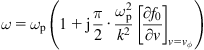
The dispersion relation for the wave in a magnetic field is thus
![]() (1.124)
(1.124)
where ωh is the upper hybrid frequency. Physical explanation of these oscillations is as follows. Similar to plasma oscillations, electrons form region of compression and rarefaction. There are two restoring forces acting on electrons, the electric field force and the Lorentz force due to presence of the magnetic field. As a result, frequency of these oscillations is larger than that of the plasma oscillations as can be seen from Eq. (1.124).
Taking into account ion motion in this analysis leads to following dispersion relation:
![]() (1.125)
(1.125)
where ωl is the lower hybrid frequency, which is the combination of the ion and electron cyclotron wave. In this case, electron and ion oscillations are coupled so that the frequency is lower than in the case of the upper hybrid frequency.
The complete dispersion equation for the magnetized plasma is typically solved numerically to obtain the propagation constant for each of the waves at an arbitrary angle with respect to the magnetic field. Typically it is presented in Clemmow–Mullaly–Allis (CMA) diagram in which dispersion ω versus k for the principal waves in magnetized plasma is plotted [22].
1.3.7 Plasma instabilities
In the previous section, we considered waves in plasma that is equilibrium unperturbed state. Particles in plasma had equilibrium (Maxwellian) velocity distribution and density, and magnetic and electric fields were uniform. In this case, there is no free energy available and thus waves were excited by external means. In this section we will consider situation in which plasma is not in a perfect equilibrium and thus free energy is available to excite waves and drive system to an unstable state. Instabilities can be classified by the free energy that drives their development. Here we will follow classification that was proposed by Chen [21].
1. Streaming instability: The beam of energetic particles travels through the plasma. The drift energy is utilized to excite waves. An example of this instability is the two-stream instability.
2. Rayleigh–Taylor instabilities: In this case, instability is driven by presence of the density gradient and external nonelectromagnetic forces.
3. Universal instabilities: Even if plasma is in the equilibrium, plasma pressure gradient leads to the expansion. All confined plasmas defuse slowly due to particle collisions. This expansion energy can drive the instability. This kind of instability always present in plasma and this is why they called universal. A known example is the drift instability.
4. Kinetic instability: If the velocity distribution of plasma particle is not Maxwellian, there is always deviation from equilibrium and the instability can be driven by energy distribution anisotropy.
In the following section, we consider a particular example of streaming instability, namely, the two-stream instability. For more details analysis of the waves in plasmas and plasma instabilities, we refer to several textbooks [21,22].
1.3.7.1 Two-stream instability
Consider cold plasma with Te=Ti=0 and without a magnetic field, i.e., B=0.
The linearized equations of motion for ions (Eq. (1.93)) and electrons (Eq. (1.100)) will have the following form:
![]() (1.126)
(1.126)
![]()
where v0 is the velocity of electron stream. Electrostatic wave is considered:
![]() (1.127)
(1.127)
Employing the form (1.127) for the electric field in Eq. (1.126), we arrive at
![]() (1.128)
(1.128)
Solving this equation for vi1 yields
![]() (1.129)
(1.129)
After employing the electric field in the form (1.127), the equation for electron motion will have the following form:
![]() (1.130)
(1.130)
Solving this equation for the electron velocity
![]() (1.131)
(1.131)
Under considered conditions, the ion continuity equation is
![]() (1.132)
(1.132)
One can solve this equation for the ion density:
![]() (1.133)
(1.133)
Electron continuity equation is
![]() (1.134)
(1.134)
After linearization, this equation becomes
![]() (1.135)
(1.135)
Solving this equation for the electron density yields
![]() (1.136)
(1.136)
We can now plug Eqs (1.133) and (1.36) into the Poisson’s equation:
![]() (1.137)
(1.137)
which looks like:
![]() (1.138)
(1.138)
The dispersion relation is thus
![]() (1.139)
(1.139)
Let us now examine whether these oscillations are stable or they can become unstable. To this end we will find a root of ω assuming that it is a complex variable, i.e.,
![]() (1.140)
(1.140)
Taking into account Eq. (1.140), the electric field becomes
![]() (1.141)
(1.141)
Let us analyze the dispersion equation (1.139) using the following normalized variables:
![]()
The dispersion equation becomes
![]() (1.142)
(1.142)
The solution of Eq. (1.142) can be shown graphically in Figure 1.24.
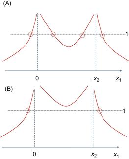
The function F(x1,x2) is shown with two possible cases considered. It can be seen that in Figure 1.24A, there are four real roots, while in Figure 1.24B, there are two real and two imaginary roots with one of the roots being positive. Thus for sufficiently small kvo plasma becomes unstable. In the case of a given v0, plasma is unstable for long-wave oscillations.
The maximum growth rate can be estimated from Eq. (1.139) for m/M![]() 1:
1:
![]() (1.143)
(1.143)
This instability is sometimes called the “Buneman” instability. Physics of this instability can be explained as follows. The natural electron frequency is ωp, while the ion frequency is Ωp=(m/M)0.5ωp. Because of the Doppler shift of oscillations moving with electrons, these two frequencies could be equal for given kvo. As a result, the energy can be transferred from electrons to ions providing conditions for wave growth.
1.3.7.2 Kinetic instabilities
So far we considered instabilities and waves using the fluid approximation and as such assuming that particles in plasma obey equilibrium (Maxwellian) velocity distribution. However, in many cases, the energy distribution function of the particles in plasmas can deviate from Maxwellian distribution due to imbalanced conditions. The deviation from the equilibrium distribution can be maintained due to rare collisional events in rarefied plasmas.
Let us consider small deviation from equilibrium as follows:
![]() (1.144)
(1.144)
where f0(r,v,t) is the Maxwellian distribution function. Linearized, the collisionless Boltzmann equation leads to
![]() (1.145)
(1.145)
In accordance with previous analysis, we assume
![]() (1.146)
(1.146)
By substituting Eq. (1.146) into Eq. (1.145), we arrive at
![]() (1.147)
(1.147)
Solving Eq. (1.147) for f1 yields the following:
![]() (1.148)
(1.148)
Using the Poisson equation, the electric field E1 can be expressed as
![]() (1.149)
(1.149)
After substituting f1 and some algebra, dispersion relation can be obtained:
![]() (1.150)
(1.150)
One can see that integral (1.150) has a singularity. Landau treated this integral using the contour integration. By doing that, one can arrive at
 (1.151)
where vϕ=(ω/k) is the phase velocity.
Taking into account that the fo is the Maxwellian distribution function, one can obtain expression for the decay rate of this oscillations of distribution function.
![]() (1.152)
(1.152)
Since imaginary part is negative, wave is damping. This effect is called Landau damping.
Note: This is very surprising result because the wave is damped without collisions! It was first discovered by Landau [23] theoretically and then was confirmed experimentally by Malmberg and Wharton [24].
In order to understand the underlying physical mechanism, let us consider the electron velocity distribution function as shown schematically in Figure 1.25. In particular we are interested in particles with velocities near the phase velocity as shown in Figure 1.25. The particles with velocity close to the phase velocity of the wave travel with wave and thus can interact efficiently with the wave. If decreasing branch of the velocity distribution function is considered as shown in Figure 1.25, it can be seen that more particles have velocity smaller than the phase velocity (slow electrons). In other words energy, more particles have energy smaller than the wave energy than particles with energy larger than the wave energy. In this case, the wave energy is transferred into particles and thus wave is damping.

Figure 1.25 Electron distribution function and distortion of a Maxwellian distribution function near phase velocity due to Landau damping.
Using analogy with waves in the sea can provide intuitive explanation of the Landau damping. In this case, we consider the particles as surfers trying to catch the wave as shown in Figure 1.26. If the surfer is moving on the water surface at a velocity slightly less than the waves, he will eventually be caught and pushed along the wave (and will gain the energy), while a surfer moving slightly faster than a wave will be pushing on the wave as he moves uphill (and will lose the energy to the wave).

In summary, in this section, we considered wave propagation in the plasma and plasma–wave interactions. In particular, we considered Langmuir wave, ion sound wave, as well as waves in a magnetic field. Plasma instability associated with either drift or gradients was considered for conditions relevant for some aerospace applications. In addition, we consider kinetic effect such as Landau damping which is relevant for rarefied plasmas considered in subsequent chapters.
1.4 Plasma–wall interactions
This section describes phenomena appeared in plasma–wall regions including electrostatic sheath formation and associated with particle–wall interaction, heat flux formation from the plasma, electron emission, and vaporization.
1.4.1 Plasma–wall transition: electrostatic phenomena
Typically laboratory plasmas contact the wall and such interaction leads to formation of the transitional region. The plasma-wall transition is characterized by subregion having different space charge, electric field particle densities, and velocities. Sheath is the strongly space charged subregion that appears as a result of charge particle separation in the immediate vicinity of the wall of a strong electric field. The subdivision of a discharge into a plasma bulk region and a sheath was introduced by Langmuir and Tonks [25]. Sheath region solution requires boundary conditions at the plasma–sheath interface assuring the monotonic potential distribution. Such boundary condition at the interface was considered by Bohm [26] who formulated a criterion for a stable potential distribution inside of the sheath, known as a Bohm criterion for the ion speed at the mentioned interface. It should be pointed out that while condition for the ion velocity is established, the sheath thickness is not well defined.
The transition between quasi-neutral plasma and collisionless sheath is continuing to be a subject of great interest having both academic and practical importance [27–30]. A controversial discussion on this subject was intensified in the last decade [31–36]. One of the major discussed issues is how solution of quasi-neutral plasma and sheath can be joined together using either matching or patching mathematical technique. Matching means that all variable and their derivatives are continuous; patching require continuity of variables only. A comprehensive review which addresses the problem of joining plasma and sheath solution over a wide range of physical conditions was reported by Franklin [37].
In general, the modern computer technique allows obtaining the continuity solutions without subdivisions of the plasma–wall transition layer. However, there are physical situations in which plasma region required multicomponent and multidimensional analysis, while sheath region can still be treated as a one-dimensional system. Moreover, sheath analysis has significant methodical value of illustrating the physics of the plasma–wall transition. For example, the low-pressure discharges in microdevices and plasma thrusters were studied with essentially two-dimensional plasma region and one-dimensional sheath region [38]. Thus it is often convenient to obtain the plasma and the sheath solutions separately. The essence of the Bohm criterion and an example of a solution in plasma–sheath regions will be analyzed below.
1.4.1.1 Condition for stable sheath: Bohm criterion
Let us discuss the necessity of certain ion velocity at the sheath edge to have a monotonic potential distribution in the sheath. To this end, a collisionless sheath with quasi-neutral presheath can be considered schematically presented in Figure 1.27. The ion velocity at the sheath edge can be calculated using the equations of energy particle flux conservation[69]:
![]() (1.153)
(1.153)
where φ(x) is the potential distribution function, M, V, and Cs are the ion mass, velocity, and sound velocity, respectively. The left-hand side corresponds to the ion kinetic energy evaluated in the sheath at boundary x=0.
Ion continuity equation can be written as
![]() (1.154)
(1.154)
where n(x) is the density distribution function. From Eqs (1.153) and (1.154), one can derive:
![]() (1.155)
(1.155)
According to Eqs (1.153) and (1.154), the ion density distribution is therefore:
![]() (1.156)
(1.156)
Electrons obey the Boltzmann distribution:
![]() (1.157)
(1.157)
Plasma is quasi-neutral at the presheath–sheath, i.e., nes=nis=ns, where nes and nis are, respectively, the electron and ion densities at the sheath edge.
The Poisson’s equation:
![]() (1.158)
(1.158)
Substituting expressions (1.156) and (1.157) for the ion and electron densities in the Poisson’s equation:
 (1.159)
Considering the one-dimensional approach, Eq. (1.159) can be expressed as
 (1.160)
Equation for the electric field can be obtained by first integration of Eq. (1.160):

where ![]() and C is the constant of integration.
and C is the constant of integration.
Using the following boundary conditions at x=0:
![]()
it can be obtained:
![]() (1.161)
(1.161)
Using Eq. (1.161), the equation for the electric field becomes
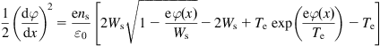 (1.162)
The Taylor expansion near the sheath edge reads
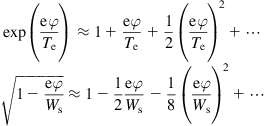 (1.163)
To reach the stable monotonic potential distribution in entire sheath region, the following condition at the external boundary of the sheath should be fulfilled:
![]() (1.164)
(1.164)
Consider potential near the sheath edge, eφ/Te<1. Thus high-order terms (such as (eφ/Te)2 and higher) can be neglected. After some algebra, Eq. (1.162) becomes
![]() (1.165)
(1.165)
This leads to the following condition, which is known as Bohm criterion:
![]() (1.166)
(1.166)
1.4.1.2 Monotonic solution for sheath–presheath region
Here we illustrate the sheath and in a more general sense plasma–wall interface by considering solutions of a quasi-neutral plasma and a sheath separately. By employing the patching technique, we will illustrate how to obtain the monotonic solution for entire plasma–wall transition region.
The fluid-based approach is considered below to illustrate the sheath problem and its solution. Schematically the transition regions are shown in Figure 1.27. According to Langmuir’s analysis [25], the ions are accelerated toward the Bohm velocity in a plasma region with a relatively weak electric field and this region called as presheath extends from the sheath into the quasi-neutral plasma volume. The electric field, thus, becomes a continuous function increasing in the sheath from a boundary value up to a maximal value at the wall. This boundary field can be obtained considering a model for the presheath region. The position of the sheath–plasma interface is determined by patching the electric field, ion velocity, and potential. Thus a relationship between the ion velocity and the electric field at the presheath–sheath interface should be determined to choose these parameters as boundary conditions for a sheath region solution.

The procedure described involves the following conditions: (i) the degree of the quasi-neutrality violation near the presheath edge that may affect the solution will be estimated; (ii) potential distribution is spatially monotonic in all regions, and (iii) continuity of the electrical field and potential at the sheath–presheath interface.
1.4.1.3 Mathematical formulation
Let us consider the governing equations to describe the problem including the plasma, the sheath, and the sheath–presheath interface. The plasma flow in the quasi-neutral plasma region is considered in the fluid approximation. Ion mass and momentum conservation taking into account and assuming that the electrons obey the Boltzmann distribution:
![]() (1.167)
(1.167)
![]() (1.168)
(1.168)
![]() (1.169)
(1.169)
where ne and ni are electron and ion densities, respectively, νi is the ionization collision frequency, and νc is the charge-exchange collision frequency. In order to obtain main dependencies, we assume that collision frequency is constant, Zi is the ion charge state (only single ionized ions will be considered, Zi=1), Pi is the ion pressure (cold ions are assumed, so Pi=0) and E=−dφ/dx is the electric field and φ is the potential. The potential is distributed according to Poisson’s equation:
![]() (1.170)
(1.170)
The system of equations (1.167)–(1.170) has following boundary conditions:
At the symmetry axis (as shown in Figure 1.28) (x=0), φ=0, dφ/dx=0, and ne=ni=no.

Figure 1.28 Schematics of the plasma–wall transition regions (not to scale). Ion velocity, Vo (normalized by Cs), and electric field, Eo (normalized by E*), distribution in the neighborhood of the presheath–sheath interface. The broken line shows the potential distribution in the sheath after patching.
The above system of equations is solved separately for the quasi-neutral collisional plasma region (presheath) and for collisionless space charge region (sheath). Finally it will be described how to patch these two solutions.
1.4.1.3.1 Presheath (quasi-neutral region, ne=ni)
Naturally we normalize these equations with u=Vi/Cs, χ=x/λc, η=eφ/kTe, where no is the plasma density at the plasma center, λc=Cs/(νc+νi), Cs=(kTe/m)1/2. The normalized system of equations (1.167)–(1.169) with quasi-neutrality assumption can be easily reduced to the following system of equations:
![]() (1.171)
(1.171)
![]() (1.172)
(1.172)
where α=(vi/(vi+vc)). This system of equations and the boundary conditions determine the solution up to point u→1, where a large electric field and therefore a certain deviation, Δn=ne−ni, from the quasi-neutrality condition can be expected. Using the potential distribution (from Eq. (1.170)), this deviation can be described as follows:
![]() (1.173)
(1.173)
where ψ=(λD/λc) and λD is the Debye length at the plasma axis (x=0) and λc is the collision mean free path. The relationship between Vo and Eo (Vo is the ion velocity normalized by Cs and Eo is the electric field normalized by E*=Te/eλD) can be obtained from Eqs (1.171) and (1.172). A monotonic sheath solution can be obtained by patching or matching the solution with normalized electric field and normalized velocity at the sheath–presheath interface.
1.4.1.3.2 Sheath
This is the plasma region where the volume space charge is relatively large and the plasma cannot be considered as a quasi-neutral substance. A collisionless sheath is assumed, i.e., νi=νc=0. This allows description of the ion density distribution in the sheath using a simple form of the mass and momentum conservations (Eqs (1.167) and (1.170)) as
![]() (1.174)
(1.174)
The electron density distribution in the sheath is still determined by the Boltzmann equilibrium:
![]() (1.175)
(1.175)
where ns is the density, ηo is the potential, and Vo is the ion velocity at the sheath–presheath interface. The potential distribution in the sheath is calculated from the following normalized Poisson equation:
![]() (1.176)
(1.176)
1.4.1.3.3 Direct numerical solution of the sheath–presheath regions
The above described approach can be compared with a direct numerical solution of the entire plasma–wall interface. This solution describes the entire transition region between the plasma and the wall without division between a quasi-neutral part and a sheath and taking into account collisions. Let us normalize Eqs (1.167)–(1.170) for the entire transition region from the plasma to the wall:
![]() (1.177)
(1.177)
![]() (1.178)
(1.178)
![]() (1.179)
(1.179)
![]() (1.180)
(1.180)
where ψ=(λD/λc), Ne=ne/no; Ni=ni/no. Below, the exact solution will be compared with the approximate patching solution. Before the solution will be presented, the relationship between velocity and electric field at the sheath edge is analyzed in the next section.
1.4.1.4 Monotonic potential distribution in the sheath
Consider Poisson equation for the sheath potential distribution in dimensionless form:
![]() (1.181)
(1.181)
The first integration of Eq. (1.181) in the vicinity of the sheath boundary with nonzero electric field at the sheath boundary, Eo=−(dη/dχ)o, gives
![]() (1.182)
(1.182)
where ηs is the potential at some point in the sheath including region close to the sheath edge. For the purpose of simplifying analyses, we assumed here that potential at the sheath boundary equals zero, η0=0. All parameters (density, velocity, and potential) are normalized by their values at the sheath edge. Near the sheath edge, one can make a series expansion in the small parameter ηs![]() 1:
1:
 (1.183)
Neglecting small terms in the expansion with order higher than ![]() reduces Eq. (1.182) to the following:
reduces Eq. (1.182) to the following:
![]() (1.184)
(1.184)
The condition for the monotonic potential distribution in the sheath would be that the right-hand side of Eq. (1.184) is positive. This condition has the following form:
![]() (1.185)
(1.185)
Obviously, Eq. (1.185) has no real solution in the sheath if Vo<1 and Eo=0. Therefore, for Eo=0, the potential distribution in the sheath is monotonic only when Vo≥1, i.e., with Bohm condition.
Equation (1.185) has real solution (the monotonic potential distribution) in the sheath for Vo<1 when Eo>0. The requested Eo that supports the monotonic potential distribution was obtained from the numerical solution of the sheath equations and shown below.
To get more understanding of the above points, let us analyze the solutions of Eq. (1.182) as a function of two variables η and dη/dχ, i.e., potential–electric field plane. In this case, the solution of Eq. (1.182) can be represented as dependences with parameter of ![]() Mathematical analysis of Eq. (1.182) in (η–dη/dχ) plane shows that the solutions could be centers or saddles. Centers solution corresponds to the periodic behavior of the mathematical system (oscillations), while saddles solution corresponds to spatially monotonic behavior.
Mathematical analysis of Eq. (1.182) in (η–dη/dχ) plane shows that the solutions could be centers or saddles. Centers solution corresponds to the periodic behavior of the mathematical system (oscillations), while saddles solution corresponds to spatially monotonic behavior.
The contours of ![]() directly computed from Eq. (1.182) are shown in Figure 1.29A. It can be seen that both saddles and centers curves of the same level of initial electric field Eo are possible and those solutions depend on the initial velocity Vo. Figure 1.29B shows that smaller
directly computed from Eq. (1.182) are shown in Figure 1.29A. It can be seen that both saddles and centers curves of the same level of initial electric field Eo are possible and those solutions depend on the initial velocity Vo. Figure 1.29B shows that smaller ![]() corresponds to centers curves, while large
corresponds to centers curves, while large ![]() corresponds to saddles curves.
corresponds to saddles curves.

Figure 1.29 (A) Level curves of ![]() for the case of Vo=0.95. Centers curves correspond to oscillatory solution, while saddles curves correspond to the monotonic solution. (B) Level curves of
for the case of Vo=0.95. Centers curves correspond to oscillatory solution, while saddles curves correspond to the monotonic solution. (B) Level curves of ![]() for the case of Vo=0.95. Centers curves correspond to oscillatory solution, while saddles curves correspond to the monotonic solution.
for the case of Vo=0.95. Centers curves correspond to oscillatory solution, while saddles curves correspond to the monotonic solution.
Recall that dependent on the boundary conditions at the sheath edge (i.e., electric field and ion velocity), spatially monotonic or oscillatory behavior of potential distribution is possible.
1.4.1.5 Solutions in plasma and sheath regions: procedure of patching
Firstly, the quasi-neutral (presheath) region (i.e., Eqs (1.171), (1.172)) is considered. The distribution of the velocity, electric field, and quasi-neutrality deviation is shown in Figure 1.30A and Figure 1.30B. The ion velocity variation in this scale length (fraction of a mean free path) is small, while the electric field and quasi-neutrality deviation noticeably increase in the presheath with distance toward the presheath edge and become singular (Figure 1.30A). As shown in Figure 1.30B, both the electric field and the quasi-neutrality deviation significantly increase when the ion velocity approaches to the Bohm velocity. This deviation becomes stronger with coefficient ψ decreasing.
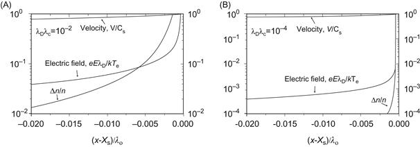
Figure 1.30 Velocity, electric field, and quasi-neutrality assessment spatial variation near the presheath edge with ψ as a parameter. Zero coordinate ((x−Xs)/λc=0) corresponds to the presheath edge, i.e., condition: V=Cs. α=1. (A) ψ=10−2 and (B) ψ=10−4.
Now let us consider the procedure of patching the presheath and the sheath solutions. The existence of the solution with spatially monotonic potential distribution in the sheath region is examined in Section 1.4.1.4. The procedure of finding the monotonic solution is as follows. Having the boundary velocity Vo and corresponded electric field Eo, the potential distribution in the sheath (Eqs (1.174)–(1.176)) is calculated. Two types of potential distribution are possible as shown in Figure 1.31. When electric field Eo is small and Vo<1, the only oscillating solution of the Poisson equation is possible. A combination of the nonzero electric field Eo and velocity Vo (if Vo<1) provides the spatially monotonic solution. These conditions are the boundary condition for the sheath.

Figure 1.31 Potential distribution in the sheath with boundary velocity as a parameter. Boundary electric field Eo corresponds to the velocity Vo in the presheath solution.
In the above described approach, the velocity Vo is searched as a minimal velocity for which spatially monotonic potential distribution in the sheath is possible.
The calculations show that when ψ increases, the ion velocity at the sheath edge is smaller than the Bohm velocity and at the same time the obtained electric field increases with ψ (Figure 1.32). However, the electric field increase coexists with the quasi-neutrality violation, as it is also shown in Figure 1.32. In the opposite limit, i.e., when ψ is small, the required velocity approaches the Bohm velocity and at the same time the electric field approaches zero. One can see that up until ψ=10−2, the level of deviation from quasi-neutrality is small (about few percent) and can be tolerated in many cases. In the case when the parameter ψ increases and approaches unity, the collisions become important in the sheath and therefore Eq. (1.174) should be modified taking into account the change of momentum by the collisions. The tendency is shown in Figure 1.32; when parameter ψ increases, the velocity significantly decreases and the Bohm criteria requirement is relaxed. Also there is an intermediate range of ψ (where 10−4<range<10−2) when the sheath can still be considered collisionless, but the sheath and presheath solutions can be patched with velocity smaller than the Bohm velocity and a nonzero electric field.
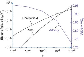
Figure 1.32 Velocity, electric field, and quasi-neutrality assessment at the patching point as a function of Debye length ratio to the collision mean free path ψ.
The accuracy of the proposed patching procedure for ψ=10−4 is compared with the continuous direct numerical solution (1.177)–(1.180) as shown in Figure 1.33, where the electric field as a function of the potential in the presheath and the sheath is shown. One can see a good agreement between continuous (direct) solution and solution using above developed patching approach.

Figure 1.33 The variation of electric field as a function of potential. α=1; ψ=10−4. The direct numerical solution of Eqs (1.177)–(1.180) is shown with dotted line. φw=−8kTe/e.
The density distribution across the sheath region shown in Figure 1.34 illustrates that two approaches (collisionless sheath-solid curve (i.e., patching) and dotted curve—direct numerical solution) produce very close results. The patching solution is obtained using the appropriate boundary conditions for ion velocity and electric field necessary for continuous distribution of these parameters at the sheath–presheath interface. The difference between those solutions is due to the fact that the collisions were neglected in the sheath solution. This implies that collisional effects in the sheath are not significant.

Figure 1.34 Ion and electron density distribution in the sheath. α=1; ψ=10−4. The direct numerical solution of Eqs (1.177)–(1.180) is shown with dotted lines. The calculated patching: velocity is Vo=0.944 and electric field, Eo=1.631·10−3.
1.4.1.6 Typical electrostatic sheath
1.4.1.6.1 Child–Langmuir sheath
A sheath with large potential bias on the wall with respect to the plasma is considered schematically presented in Figure 1.35, where “0” corresponds to the sheath edge and “s” corresponds to the wall. As a negative voltage is applied, electrons will be repelled away from the wall leading to positive sheath formation. The ions are accelerated toward the wall by the electric field of the sheath.

We can obtain the thickness of the sheath by integrating the Poisson equation (Eq. (1.170)):
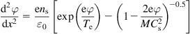 (1.186)
Setting the following boundary conditions:
![]()
The potential at the wall is chosen to be much larger than the electron temperature. In this case in most of the sheath region:
![]() and thus first term in Eq. (1.186) can be neglected. Also assuming that ni=constant=ns, the Poisson equation is then has the following form:
and thus first term in Eq. (1.186) can be neglected. Also assuming that ni=constant=ns, the Poisson equation is then has the following form:
![]() (1.187)
(1.187)
After integration of Eq. (1.187), it can be obtained a simple solution which is called ion matrix sheath.
For the electric field:
![]() (1.188)
(1.188)
The potential distribution can be obtained by integrating Eq. (1.188):
![]() (1.189)
(1.189)
Employing the boundary condition, i.e.,
![]()
at x=s,
![]()
at x=0.
Thus one can find that sheath thickness as
![]() (1.190)
(1.190)
The approach can be extended using the ion conservation equation, i.e., nivi=constant in the sheath. As it is done above, we also assume that electrons are depleted in the sheath due to high potential in comparison with electron temperature, i.e., ne![]() ni and that the ion velocity in the sheath is much higher than that at the sheath edge.
ni and that the ion velocity in the sheath is much higher than that at the sheath edge.
General equation (1.186) for the sheath is reduced to
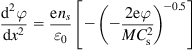 (1.191)
Following the definition of the ion current density, i.e., J0=ensCs, we can rewrite Eq. (1.191) as
 (1.192)
After integration, we arrive at
![]() (1.193)
(1.193)
Using the boundary condition φ(0)=0, it follows that constant C=0.
After some arithmetical operations:
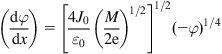 (1.194)
Second integration thus produces
![]() (1.195)
(1.195)
Using boundary condition at the wall, i.e., −φ=V0 at x=s, it is
![]() (1.196)
(1.196)
Solving this equation for the current results in
![]() (1.197)
(1.197)
This equation is well known as a Child–Langmuir law of space-limited current in a plane diode. When spacing s is fixed, the current between two electrodes can be calculated as a function of applied voltage. Child–Langmuir law is not valid when V0~Te and ion velocity at the positively charged electrode is not zero which is the case of a floating wall potential.
1.4.1.6.2 Sheath at floating wall
The potential drop across a sheath between the plasma and a floating wall can be calculated taking into account that total current to the wall must be equal to zero.
Ion current can be calculated as
![]() (1.198)
(1.198)
Electron current is calculated as
![]() (1.199)
(1.199)
As Ii=Ie, the wall potential solving Eqs (1.198) and (1.199) is
![]() (1.200)
(1.200)
1.4.1.6.3 Sheath with arbitrary ion distribution function: kinetic approach
By considering an arbitrary ion distribution function, Bohm criterion for a stable sheath can be generalized. Allen [39] demonstrated that the generalized Bohm criterion has the following form:
![]() (1.201)
(1.201)
where g(w) is the normalized ion velocity distribution function, w is the ion velocity, M is the ion mass, k is the Boltzmann’s constant, and Te is the electron temperature.
We will follow the interpretation of the condition (1.201) proposed in [40].
Ion density inside the sheath region can be calculated using the distribution function as
![]() (1.202)
(1.202)
where φs is the potential at the sheath edge and ns is the ion density at the sheath edge. After differentiating Eq. (1.202) with respect to φs, one arrives to
![]() (1.203)
(1.203)
At the sheath edge, ion density gradient becomes
![]() (1.204)
(1.204)
If we assume that electrons obey Boltzmann distribution, the electron density derivative at the sheath edge is
![]() (1.205)
(1.205)
Sheath stability is associated with requirement that electron density decreases faster than the ion density, i.e.,
![]() (1.206)
(1.206)
Let us now substitute expressions for ion and electron density gradient into Eq. (1.206):
![]() (1.207)
(1.207)
This leads us to Eq. (1.201), which is the generalized Bohm criterion in the case of arbitrary ion density distribution.
1.4.1.6.4 Sheath with secondary electron emission (SEE)
Under typical steady-state conditions considered above, the potential drop between the plasma and the wall is negative in order to repel the excess of thermal electrons (see Section 1.4.1.6.2). However, when the wall has substantial SEE, the floating potential drop may be different from that in the simple sheath. Hobbs and Wesson [41] were first to describe this situation in detail.
Considering a one-dimensional sheath model and taking into account the SEE from the wall, the electrostatic potential distribution in the sheath satisfies the Poisson equation:
![]() (1.208)
(1.208)
where φ is the potential, ne1 is the density of plasma electrons, ne2 is the density of secondary electrons, and ni is the ion density. The plasma electrons are assumed to obey the Boltzman distribution:
![]() (1.209)
(1.209)
where ne2(0) is the density of the secondary electrons at the sheath edge and no is the electron density at the sheath edge that is equal to the ion density ni(0). The ions are assumed to be cold and have at the presheath–sheath interface the energy ![]() where Vo is the ion velocity at the sheath edge and mi is the ion mass. Ions have free motion in the sheath and their density decreases according to
where Vo is the ion velocity at the sheath edge and mi is the ion mass. Ions have free motion in the sheath and their density decreases according to
![]() (1.210)
(1.210)
The current continuity equation can be written in the form
![]() (1.211)
(1.211)
where je1 is the flux of the primary electrons from the plasma (j=nV is the flux definition for all species), ji is the ion flux, and je2 is the flux of the secondary electrons. From this equation, one can obtain that
![]() (1.212)
(1.212)
where δ is the SEE coefficient determined as δ=je2/je1. We will furthermore assume that the electrons emitted from the surface are monoenergetic and freely move in the sheath. The boundary conditions for the sheath problem are the following:
![]() (1.213)
(1.213)
From the current continuity equation (Eq. (1.211)), one can calculate the potential drop across the sheath Δφw as
![]() (1.214)
(1.214)
One can see that the potential drop across the sheath decreases with the SEE coefficient. It should be noted that in this model, we have assumed that a monotonic potential distribution exists. However, when the SEE coefficient δ approaches unity, the solution in form (1.214) breaks down and when δ exceeds a critical value, a potential well forms such that a fraction of emitted electrons is returned to the wall. This happens when δ is less than 1 and it was obtained that the critical value of the SEE coefficient δ* can be calculated as
![]() (1.215)
(1.215)
From Eq. (1.215), it can be estimated that in the case of BN (commonly used dielectric material), the critical SEE coefficient is about 0.95.
1.4.1.7 Sheath in a magnetic field
Magnetic field affects the plasma–sheath transition. Schematically plasma–wall interface in a magnetic field is shown in Figure 1.36.
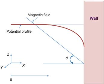
Daybelge and Bein [42] were the first to completely analyze a collisionless sheath, in which a magnetic field exists between fully ionized plasma and an infinite plane metal wall. The potential distribution in the sheath was obtained from the solution of Poisson equation, using the wall potential as a parameter and assuming a Maxwellian distribution for the charged particle velocities at the sheath–plasma edge. They obtained that sheath thickness is comparable to the ion Larmor radius in the case of negative wall potentials, whereas for positive wall potential it is reduced to the electron Larmor radius. However, Daybelge and Bein considered in their model the electrostatic sheath region only for the case LD![]() rLe, where LD is the Debye length and rLe is the electron Larmor radius. Therefore, the ionic presheath acceleration was not considered. Later, the effect of the magnetic field on the plasma presheath was studied by Chodura [43] in the collisionless limit. Plasma quasi-neutrality in the presheath and a Boltzmann distribution for the electron density were assumed in order to determine the electric field in the sheath. Chodura found that in order to satisfy the usual Bohm condition at the sheath–plasma edge, a new double-layer presheath was required. In the first double presheath region, the ions are accelerated to supersonic velocities parallel to the magnetic-field lines, which may be oblique with respect to the wall. In the second presheath region, which has the thickness of approximately the ion Larmor radius, the ion velocity vector is rotated so that the velocity normal to the wall is supersonic at the entrance to the sheath. Unlike the above-mentioned models, Riemann’s analysis of the presheath region in a plasma placed in a magnetic field also accounted for collisions[70]. The assumptions of Riemann’s fluid model are similar to those of Chodura, except that an ion collision term of constant collision frequency was added. A dependence of the potential distribution in the presheath on the magnetic field and collision frequency was found. The main effect of a strong magnetic field is to reduce the collisional presheath thickness, as it approximates now the ion Larmor radius and not the ion mean free path. Riemann also showed that in the collisional case, additional plasma presheath is not required, in contrast to the case studied by Chodura.
rLe, where LD is the Debye length and rLe is the electron Larmor radius. Therefore, the ionic presheath acceleration was not considered. Later, the effect of the magnetic field on the plasma presheath was studied by Chodura [43] in the collisionless limit. Plasma quasi-neutrality in the presheath and a Boltzmann distribution for the electron density were assumed in order to determine the electric field in the sheath. Chodura found that in order to satisfy the usual Bohm condition at the sheath–plasma edge, a new double-layer presheath was required. In the first double presheath region, the ions are accelerated to supersonic velocities parallel to the magnetic-field lines, which may be oblique with respect to the wall. In the second presheath region, which has the thickness of approximately the ion Larmor radius, the ion velocity vector is rotated so that the velocity normal to the wall is supersonic at the entrance to the sheath. Unlike the above-mentioned models, Riemann’s analysis of the presheath region in a plasma placed in a magnetic field also accounted for collisions[70]. The assumptions of Riemann’s fluid model are similar to those of Chodura, except that an ion collision term of constant collision frequency was added. A dependence of the potential distribution in the presheath on the magnetic field and collision frequency was found. The main effect of a strong magnetic field is to reduce the collisional presheath thickness, as it approximates now the ion Larmor radius and not the ion mean free path. Riemann also showed that in the collisional case, additional plasma presheath is not required, in contrast to the case studied by Chodura.
In all of the above-mentioned magnetic presheath models, a Boltzmann distribution for the electron density was assumed, and the magnetic field acted only on the ions. It should be noted that the Boltzmann distribution for the electron density is physically significant in the case of plasma flow parallel to the magnetic field. However, for plasma transport across a magnetic field, it is not obvious that this distribution will occur. It was shown by Beilis and coworkers [44,45] that the assumption about the electron distribution function influences strongly the presheath thickness. Effect of the angle of the magnetic field with respect to the wall on the presheath thickness is illustrated in Figure 1.37. One can see that when magnetic field is changed from being parallel to the wall (0°) to small incidence angle a significant change in the presheath thickness is occurred.
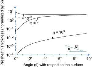
Figure 1.37 The magnetic presheath thickness (in units of the ion gyroradius) as a function of the intersection angle (90−θ, see Figure 1.36), with the electron to ion current ratio η as a parameter.
It was also shown that while density was calculated from the general system of equation (i.e., electron momentum equation that takes into account the magnetic field), the density profile does not deviate significantly from the one obtained from the Boltzmann equation as shown in Figure 1.38. However, neglecting the magnetic field term in the electron momentum equation affects the potential, density, velocity distribution in the presheath and the presheath thickness.
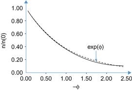
1.5 Surface phenomena: electron emission and vaporization
Plasmas in Laboratory settings are confined by physical boundaries. In this section, we consider interaction of plasma with solid materials by considering phenomena occurring at the material surface. In particular, we will consider emission of electron and material evaporation as shown schematically in Figure 1.39.

1.5.1 Electron emission
Electron emission is defined as a phenomenon of liberation of electron from the surface that is stimulated by temperature elevation, radiation, or by strong electric field. In a metallic crystal lattice, the outer electrons, valence electrons, and orbits overlap, and are shared by all the atoms in the solid. These electrons are not bound and are free to conduct current. Typically the free electron density in a metal is about 1023 cm−3. In a semiconductor, valence electrons are bound in covalent bonds. Electrons are forming a sphere in the energy space and the surface of this sphere is at the Fermi energy level. Although valence electrons are free to move inside the metal, they are bound relatively to the vacuum. A potential barrier at the surface is formed due to polarization of the electron gas according to the Shottky theory. Therefore, an image force Fim appears at the surface:
![]() (1.216)
(1.216)
where x is the distance from the surface and e is the electron charge. Thus, it is necessary to spend a certain amount of energy to enable for electron to overcome the potential barrier at the surface and be emitted from the solids. The amount of this energy is called the work function (Wf). The work functions for typical metallic emitters are presented in Table 1.1. In order to calculate the electron emission current, the electron energy distribution in the solid body should be taken in account. For example, in DC discharges, the electron current is sustained by the emission of electrons from the surface of the cathode.
Table 1.1
The Work Functions for Typical Metallic Emitters
| Element | Work Function (eV) |
| Cu (copper) | 4.4 |
| Ti (titanium) | 3.84 |
| Ag (silver) | 4.26 |
| Au (gold) | 4.8 |
| W (tungsten) | 4.5 |
According to Fermi–Dirac statistics, the electron energy distribution in the metal is
![]() (1.217)
(1.217)
where w is the electron energy and w0 is the Fermi level.
![]() (1.218)
(1.218)
where ne is the electron density and me is the electron mass.
1.5.1.1 Thermionic emission
When the metal is heated by an energy source, the surface temperature increases allowing the electrons to overcome the potential barrier at the surface. Integrating the distribution function taking the minimal energy electron as Wf:
![]() (1.219)
(1.219)
where ![]()
Presence of the electric field changes the potential distribution near the surface and lowers the potential barrier (shown in Figure 1.40) by the so-called Shottky effect reducing the work function by
 (1.220)

Figure 1.40 Schematics of the energy levels near the surface. With the external electric field, the potential barrier becomes finite.
Taking this into account the electron reflection due to quantum mechanical effect of tunneling, the expression for the current density by thermionic electron emission will have the following form:
![]() (1.221)
(1.221)
where D is the electron reflection coefficient. In general, electron reflection coefficient depends on material, surface conditions. As a result, effective thermoionic current varies significantly.
1.5.1.2 Field emission
The electron emission by electric field action is modeled assuming that surface temperature is zero. Presence of the electric field near the surface transforms the infinite thick potential distribution into a potential barrier of a finite width (Figure 1.41). As a result, electrons can escape the metal with probability determined by quantum mechanical tunneling mechanism. The current density due to the field emission, one needs to account for this quantum mechanical effect. Such treatment was done by Fowler–Nordheim, and the emission current density is given by the equation:
![]() (1.222)
(1.222)
where E is the electric field,
![]()
![]()
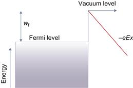
1.5.1.3 T–F emission
When the metal temperature and electric field are sufficiently high, a combined effect of thermoionic and field action was takes place. This mechanism is known as T–F emission:
![]() (1.223)
(1.223)
where eεB is the lowest potential inside the metal. According to Eq. (1.223), electron emission current is determined by two functions, namely, density of states N and emission probability D. Murphy and Good [46] performed the T–F emission analysis for some limited regions of T and E. The electron emission for wide region of T and E appropriate for conditions in a cathode spot was calculated in Ref. [47]. Results can be presented in the form of emission current density distribution as a function of energy (relative to Fermi level) of emitted electrons as shown in Figure 1.42. One can see that electrons can be emitted with energy that is lower or higher than the Fermi level dependent on electric field and surface temperature. Such general approach can recover both limits of thermoionic emission in the case of a small electric field and field emission in the case of smaller temperature.
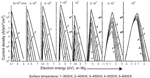
Figure 1.42 Dependence of the emission current density on the energy of emitted electrons with electric field and surface temperature as parameters (work function is 4.5 eV). Source: After Beilis [47].
1.5.1.4 Secondary electron emission
SEE is defined as a phenomenon in which primary electrons of sufficient energy induce the emission of secondary electrons by hitting the surface. The number of secondary electrons emitted per incident particle is called secondary emission yield. If the primary incident particles are ions, the effect is termed secondary ion emission. The coefficient of the SEE depends on the energy of incident electrons and the incident angle. Primary electron collisions with the surface of a target generate emissions of two main types of secondary electrons, namely, “true” secondary electrons and elastically reflected backscattered electrons. Measured electron emission yield is due to contribution of all secondary electrons. In general, SEE is higher for dielectric materials in the low-energy range (up to 100 eV) and high in the case of metal target material in the case of a kV energy range. Dawson [48] measured yields for some dielectric matrials as shown in Figure 1.43. Lucalox alumina and sapphire are both alumina, but in the preparation of this Lucalox alumina, a small amount of magnesia was added. As shown in Figure 1.2, the yields from the highly polished sapphire were a little greater at all energies. However, those from the polished Lucalox had become similar to the sapphire in their variation with primary energy.

Figure 1.43 SEE yield for dielectric materials. Source: Reprinted with permission from Ref. [48]. Copyright 1966, American Institute of Physics.
SEE yield δ(Ep) as a function of energy of the primary electrons was measured for several dielectric materials [49] as shown in Figure 1.44. One can see that SEE yield increases with energy and reaches unity at the energy of primary electrons of about 25–30 eV in the case of boron nitride.

Figure 1.44 Total yield of SEE σ(Ep) from boron nitride and quartz as a function of energy of primary electrons. Source: Reprinted with permission from Ref. [49]. Copyright 2003, American Institute of Physics.
1.5.2 Vaporization
Vaporization is the phenomenon of emission of atoms or molecules from the surface exposed to heat. In general, vaporization describes any type of phase transition from solid/liquid into a gas. Below the direct transition from solid or liquid material into the gas phase will be considered.
An important issue for many applications is the vaporization of a hot surface due to interaction with discharge plasmas. This phenomenon occurs in different devices such as ablation-controlled arcs [50], pulsed plasma thrusters [51,52], high-pressure discharges [53], vacuum arcs [54], electroguns [55], and metal evaporation by laser radiation action [56,71]. The mechanism of vaporization into vacuum was described by Langmuir relationship [57].
1.5.2.1 Langmuir model
This is the simplified model that is based on the equilibrium condition near the surface. Consider a rate at which molecules condense on a surface κν, where κ is the sticking coefficient (ratio of the flux condensed/flux striking the surface) and ν is the ablated flux. Langmuir showed that for the case of vapor for same metal, the coefficient κ=1.
On the other hand, the flux of evaporated molecules noted as μ equal to ν in the equilibrium. Taking into account that ν=(1/4)nVa, one arrives to the following rate of vaporization:
![]() (1.224)
(1.224)
The main Langmuir’s assumptions:
1. Atomic emission rate depends on surface temperature and not on the gas properties.
Despite the fact that this model is not exact in case of P∞≠0, it is widely used [58]. In the next section, more general kinetic model will be described.
1.5.2.2 Kinetic models
Anisimov [59] considered a case of vaporization of a metal exposed to laser radiation using a bimodal velocity distribution function in the nonequilibrium (kinetic) or Knudsen layer. The main result of this work is the calculation of the maximal flux of returned atoms to the surface, which was found to be about 18% of the flux of vaporized atoms. This result was obtained under the assumption that the atom flow velocity is equal to the sound velocity at the external boundary of the kinetic layer. Schematically this layer is shown in Figure 1.45. In many physical situations, however, the expansion of the vapor is not by the sound speed since there is dense plasma in the volume discharge. The vaporization phenomena in case of plasma presence at the metal surface with velocity lower than the sound speed were developed by Beilis [60–62] who considered metal vaporization into discharge plasmas in the case of a vacuum arc cathode spot. He concluded that the parameters at the outer boundary of the kinetic layer are close to their equilibrium values and that the velocity at the outer boundary of the kinetic layer is much smaller than the sound velocity.

The nonequilibrium layer close to the evaporating surface can be also modeled using the particle method known as direct simulation Monte Carlo (DSMC) [63]. This method solves numerically the Boltzmann equation allowing calculation of the thickness of the nonequilibrium layer. Below the numerical results will be compared with the results of above-mentioned analytical approach for the case when the vapor velocity at the outer boundary of the kinetic layer is given as a parameter.
1.5.2.3 Model of the nonequilibrium layer
1.5.2.3.1 DSMC particle approach
In the nonequilibrium layer near the surface, there are collisions between particles that eventually lead to change of the velocity distribution function. The DSMC method uses particle motion and collisions to perform a simulation of gas dynamics under nonequilibrium conditions. Each particle has spatial and velocity coordinates. Collision approach between particles is based on a probability model developed from the kinetic theory and commonly used in DSMC [64].
To perform the DSMC simulation, we have to specify conditions at two boundaries (see Figure 1.45). At the evaporating surface with density no and temperature To, the velocity distribution function for emitted particles is in the equilibrium form [59]:
![]() (1.225)
(1.225)
At the outer boundary of the kinetic layer, the distribution function for particles is assumed to be
![]() (1.226)
(1.226)
where U is the velocity at the outer edge of the Knudsen layer as shown in Figure 1.45, n1 is the density, and T1 is the temperature at the outer boundary. These boundary conditions are supplemented by using an empirical relation between To and no.
The DSMC model employed has the following strategy. Uniform cells with size of 0.5λ are employed and time step Δt=0.3λ/Vm,s [64], where λ and Vm,s=(2kTo/m)0.5 are the molecular mean free path and the most probable thermal speed at the ablated surface. Molecules enter the flow field successively from the surface due to evaporation and from the outer boundary due to Maxwellian velocity distribution that allows particle velocities in negative direction. Using the above assumed distribution functions at the surface and at the external boundary (Eq. (1.226)), we can calculate the flux of molecules entering from the surface, Gs, and from the outer boundary of the layer, Gb, as follows:
![]() (1.227)
(1.227)
![]() (1.228)
(1.228)
where α=U/(2kT1/m)0.5. The molecular interaction is described by the variable hard-sphere (VHS) model [62]. The VHS model is employed to select molecular collision pairs from cells and to distribute the postcollision velocities. This model assumes that the scattering from molecular collision is isotropic in the center of mass frame of reference. Both boundaries (wall and outer boundary of the kinetic layer) are assumed to be perfectly absorbing. The flow will arrive at a steady state when the sum of Gs and Gb is exactly balanced by the flux of molecules leaving from the outer boundary or sticking on the surface:
![]() (1.229)
(1.229)
where Gr is the flux of the particles returned to the surface during the time step and Gf is the flux of the particles crossing the outer boundary of the layer.
The location of the outer boundary was determined as a part of the solution. The parameters at the outer boundary (n1 and T1), the evolution of the velocity distribution function inside the kinetic layer, and the flux of returned particles are calculated as a function of the outer boundary location of the layer with given velocity U at this boundary as parameter.
1.5.2.3.2 Analytical approach
Let us consider the analytical approach, where the vapor parameters T1 and n1 at the outer boundary can be obtained using integral relations for the nonequilibrium layer. This means that the problem is reduced to integration of the conservation equations of mass, momentum, and energy across the layer [59,65]. We consider a nonequilibrium layer (thickness of about a mean free path λ) adjacent to the surface (as shown in Figure 1.45), where the velocity distribution function of the evaporated molecules reached equilibrium by the rarefied collisions with the background heavy particles and furthermore the vapor flow is described by a hydrodynamic approach. We have used Anisimov’s assumption [59] that the velocity distribution function for the returned particles (vx<0) is βf1(v), where β is the proportionality coefficient. The relations of the heavy particle parameters at the outer boundary of the kinetic layer are
![]()
![]() (1.230)
(1.230)
![]()
where do=m/2kTo, d1=m/2kT1, erfc(α)=1−erf(α), erf(α) is the error function. The system of equation (1.230) is obtained using the conservation laws of mass, momentum, and energy across the layer [59]. The flux of returned particles at the outer boundary was obtained calculating the parameters of the kinetic layer in the form
![]() (1.231)
(1.231)
The system of equation (1.229) has four unknowns and therefore the solution can be found having one unknown as a parameter, which is the velocity U at the outer boundary of the kinetic layer in our case.
1.5.2.3.3 Examples of Knudsen layer calculation
The returned atom fluxes calculated according to DSMC and the analytical approaches with the thickness of the kinetic layer as a parameter are shown in Figure 1.46.
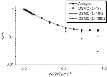
Figure 1.46 Comparison of the analytic and DSMC return flux as a function of velocity V1 with the distance of location of the outer boundary of the kinetic layer L as a parameter. Reprinted with permission from Ref. [65]. Copyright 2001, American Institute of Physics.
One can see that in the case of nomalized velocity ≤0.5 (Figure 1.46), all results agree well. This is the case when the thickness of the nonequilibrium layer is about one mean free path. In the case when evaporation occurs at about the sound velocity at the outer boundary, the DSMC calculations approach the analytical value at a layer thickness of ~10–20 mean free paths.
The calculated backflux (J−/J+) dependence on distance inside the layer is presented in Figure 1.47. It can be seen that the flux of the returned molecules depends upon the distance from the evaporating surface where the external boundary is placed. Thus, up to a layer thickness of about 20 mean free paths, the flux changed strongly and then it is saturated. Recall that varying of the position of the external boundary can be viewed as the method to find the thickness of the Knudsen layer. In this particular example, one can see that it is about 20 mean free paths. Thus one can determine the DSMC calculation predicts a 16% flux of returned particles, which is very close to the analytical result of 18%. The reason for this difference can be understood by analyzing the velocity distribution function of returned particles in the DSMC calculation. Let us now consider the velocity distribution.
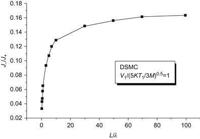
Figure 1.47 The DSMC calculated return flux as a function of the distance of location of the outer boundary of the kinetic layer L in the case of sound velocity at the boundary 1. Reprinted with permission from Ref. [65]. Copyright 2001, American Institute of Physics.
The velocity distribution functions calculated according to DSMC and the analytical approximation of βf1(v) for the sound velocity at the outer boundary are shown in Figure 1.48. DSMC distribution function agrees well with the analytic approximation when the velocity at the outer boundary of the kinetic layer is small as shown in Figure 1.48B. Therefore, the calculated flux of returned particles is also found to be in good agreement with the analytical result.

Figure 1.48 Variation of the velocity distribution function of the returned particles near the wall with the distance of location of the outer boundary of the kinetic layer L as a parameter. Reprinted with permission from Ref. [65]. Copyright 2001, American Institute of Physics.
The evolution of the particle distribution function within the Knudsen layer is shown in Figure 1.49. One can see that the velocity distribution function approaches a shifted Maxwellian at a distance of several mean free paths from the surface. The drift velocity slightly increases with further distance from the evaporating surface.
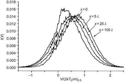
Figure 1.49 Variation of the velocity distribution function normal to the surface component with the distance from the evaporated surface as a parameter. Reprinted with permission from Ref. [65]. Copyright 2001, American Institute of Physics.
The results of calculation of the analytic system of equations 1.230 are presented in Figure 1.49 with the normalized velocity U as a parameter. The temperature T1, density n1, and the flux of returned particles J− all decrease as the velocity at the outer boundary of the kinetic layer increases. In the limiting case of the sound velocity, the flux of returned particles is equal to 18% as was obtained by Anisimov [59]. In this case, the analytically predicted flux of returned particles is larger than that obtained by numerical simulations (16%, see Figure 1.47). It should be pointed out that the dependence of the flux of returned particles J− on the velocity V1 has a minimum near the sound speed (see Figure 1.50). The minimum corresponds to the sound speed with adiabatic index 1.3, i.e., the distribution function of the returned particles is proportional to the distribution function at the outer boundary of the kinetic layer [58] (Figure 1.50). Although Figure 1.49 shows results for velocities larger than the sound speed for methodic purposes, one should note that solution with velocity higher than the sounds speed is not physical since there is no mechanism of supersonic acceleration in the model described.

Figure 1.50 Temperature, density, and returned flux at the outer boundary of the kinetic layer as a function of velocity at the outer edge of the Knudsen layer. Reprinted with permission from Ref. [65]. Copyright 2001, American Institute of Physics.
1.5.2.3.4 Ablation of the Teflon into discharge plasma
It was shown in the previous section that the velocity at the outer boundary of the kinetic layer strongly affects the kinetic layer parameters. To find the velocity V1, we apply the mass and momentum conservation equations for heavy particles in the hydrodynamic region (assuming a single fluid model) [66] between boundaries 1 and 2 as shown in Figure 1.51.

Assuming weakly ionized plasma in the hydrodynamic layer, the integration of the mass and momentum conservation equations yields the following relations between parameters at boundaries 1 and 2:
![]() (1.232)
(1.232)
![]() (1.233)
(1.233)
Combination of these two equations yields the following expression for the velocity at the outer boundary of the kinetic (Knudsen) layer:
![]() (1.234)
(1.234)
This equation makes it possible to calculate the velocity at boundary 1 and therefore to calculate the ablation rate that is proportional to V1n1. The system of equations is closed if the equilibrium vapor pressure can be specified. In the case of Teflon, the equilibrium pressure formula is used:
![]() (1.235)
(1.235)
where P=n0kT0 is the equilibrium pressure, and Pc=1.84×10¹⁵ N m2 and Tc=20 815 K are the characteristic pressure and temperature, respectively [67]. The solution of the problem depends upon plasma density n2, plasma temperature T2, and surface temperature T0. The parameters n2, T2 are determined by the bulk plasma flow. It was estimated from various experiments that, under typical operation conditions of a pulsed plasma accelerator, the plasma density near the Teflon surface is about 1021–1024 m−3, the plasma temperature is about 1–4 eV, and the Teflon surface temperature T0 is about 900–1000 K [67].
Ablation rate contours in the plane with the plasma density and Teflon surface temperature as the coordinates are displayed in Figure 1.52. The same ablation rate that can be found in the high- and low-density range corresponds to the solution of the problem with small and large velocities at the outer boundary of the kinetic layer, respectively. There is no solution for the ablation rate in regions above the curve with ablation rate equal to zero. This region in the n2–T0 plane corresponds to the case when the right-hand side of Eq. (1.234) is negative. The physical meaning of these results can be explained as follows. In the ablation-controlled discharge, the plasma density in the bulk is determined by the rate of ablation from the surface.

Figure 1.52 Contours of ablation rate in the plasma density (n2)–Teflon surface temperature (T0) plane.
In the case of small surface temperature, one can expect a smaller ablation rate and therefore high plasma densities in the discharge cannot be generated.
It is important to note that this model predicts the dependence of the ablation rate on the plasma bulk density, electron temperature, and the surface temperature. It is also found that the flow velocity at the outer boundary of the kinetic layer (that determines the ablation rate) is smaller than the sound velocity under typical conditions.
1.5.2.3.5 Outlook on evaporation analysis approached
Two kinetic approaches, numerical method DSMC and analytical approach, were employed to describe the particle parameters in the nonequilibrium kinetic layer near the evaporating surface. DSMC approach makes it possible to determine the thickness of the kinetic layer and the evolution of the particle distribution function within the layer. The layer thickness, the vapor density, and temperature in the kinetic layer adjacent to the evaporating surface depend upon the velocity at the outer boundary of the layer. The thickness of the kinetic layer increases with the particle velocity at the outer boundary of the layer and vary from a few mean free paths λ for relatively small velocity up to about 10–20λ in the case of the evaporation with sound speed.
The flux of returned particle calculated using analytical model agrees well with that calculated by DSMC approach over a wide range of velocity at the outer boundary of the layer. The present model can be used for calculation of the evaporation rate of the heated surface by interacting with plasmas. The free parameter of this model, the velocity at the outer boundary of the layer, can be determined by coupling this model with a model of the hydrodynamic layer and the plasma bulk as shown in Section 1.5.2.3.4.
Homework problems
Section 1
1. Debye length
A conductive sphere of radius a is immersed in an infinite uniform quasi-neutral plasma having density no, electrons in thermal equilibrium at temperature Te, and ions in thermal equilibrium at temperature Ti. Only single charged ions are presented. A small negative DC potential |V0|![]() Ti, Te is applied to the sphere.
Ti, Te is applied to the sphere.
a. Start from Poisson’s equation in spherical coordinates and using Boltzmann’s relation for both the electrons and ions derive expression for potential distribution.
b. Find expression for Debye length and show that Debye length is determined mainly by the temperature of the colder species.
c. Calculate Debye length for arc discharge plasma having electron density of about 1014 m−3 and electron temperature of about 1 eV and ion temperature of 0.1 eV.
Note 1: In spherical symmetry: ∇2φ=(1/r)d2(rφ)/dr2
2. Plasma oscillation
Compute plasma frequency for the following cases:
a. Vacuum arc with electron density of about 1021 m−3.
b. Hall thruster with electron density of about 1017 m−3.
c. Cold plasma with electron density of about 1020 m−3.
3. Estimate whether following ionized gases are plasmas according to conventional definition (i.e., quasi-neutrality) if characteristic size of the system is:
a. Interstellar space area (10 km)
b. Magnetic fusion device (1 m)
c. Internal confinement fusion (1 mm).
4. Compute the pressure (in atmospheres) exerted by arc plasma on its chamber. Assume that plasma is in equilibrium, i.e., Te=Ti=Ta=3000 K, n=1021 m−3. Ideal gas assumption can be employed.
Section 2
1. Ionization cross section
Plot ionization coefficient as a function of electron temperature (in eV) for nitrogen plasma. Ionization potential for nitrogen is 14.5 eV. Consider Te range 1–10 eV.
2. Plasma equilibrium
Calculate electron density of helium plasma in arc discharge at 0.1 atm as a function of electron temperature. Assume that gige/ga=2. Consider range of electron temperature 1–5 eV.
Note: LTE can be assumed.
3. Plasma composition
Calculate electron density of nitrogen–argon mixture. Pressure is 1 atm and ratio of partial pressures of nitrogen to argon is 0.5. Consider conditions for problem #2.
Section 3
1. Calculate the skin depth of electromagnetic wave in copper and iron material as a function of frequency. Consider frequencies in 10 kHz–1 MHz range.
2. Waves in plasmas. Consider plasma with density of about 1018 m−3 and electron temperature of about 5 eV. Plot the dispersion relation for electron plasma wave and ion plasma wave. Comment on results.
3. Calculate upper-hybrid and low-hybrid frequencies of arc discharge plasma having electron temperature 2 eV and electron density of about 1021 m−3. Plot dependence of both frequencies as a function of a magnetic field which is less than 1 T. Comment on results. What is the lower limit of magnetic field for low-hybrid frequency?
Note: Characteristic size of arc is 0.01 m.
4. A plasma consists of two uniform streams of ions with velocities Vx and −Vx and densities 1/3n0 and 2/3no. The neutralizing unmobile electron fluid has density no. Derive a dispersion relation for instabilities in this system.
Section 4
1. Calculate the floating potential on the probe in contact with Argon plasma with electron temperature of about 10 eV. How floating potential will change in presence of secondary electron emission (yield is about 0.4).
2. Consider hydrogen ion diode with interelectrode distance of about 2 mm. The applied voltage is −1000 V. Calculate the ion current density in the diode.
3. Consider sheath between the quasi-neutral helium plasma having electron density of about 1018 m−3 and electron temperature of about 2 eV and the floating wall. Calculate the electron density at the wall. What is the ion velocity at the wall.
Section 5
1. Calculate the electron current density due to thermoionic emission from the copper electrode as a function of surface temperature in the range of 1500–4000 K.
2. Equilibrium vapor pressure for copper (in mmHg) can be estimated as:
P=exp(A−(B/T)), where A=9.232; B=1.726×10⁴.
Calculate ablation rate using the Langmuir formula in the case of surface temperature of about 2500 K.
3. Compare the ablation rate calculated by Langmuir formula with the one predicted by the kinetic model. Use assumption that the normalized velocity at the edge of the Knudsen layer is about 1. Consider copper surface and surface temperature in the rage of 2000–4000 K.
4. Calculate contribution of the Shottky effect on the thermionic current in the case of titanium electrode. Consider surface temperature in the rage of 2500–4000 K and electric field in the rage of 107–109 V/m.
References
1. H.D. Mott-Smith, History of “Plasmas”, Nature, 233 (1971) 219.
2. Lawson JD. Some criteria for a power producing thermonuclear reactor. Proc Phys Soc B. 1957;70:6.
3. Fridman G, Friedman G, Gutsol A, Shekhter AB, Vasilets VN, Fridman A. Applied plasma medicine. Plasma Proc Polym. 2008;5:503–533.
4. Kong MG, Kroesen G, Morfill G, et al. Plasma medicine: an introductory review. New J Phys. 2009;11:115012.
5. MsscCaig CD, Rajnicek AM, Song B, Zhao M. Controlling cell behavior electrically: current views and future potential. Physiol Rev. 2005;85:943–978.
6. Stoffels E, Kieft IE, Sladek REJ, van den Bedem LJM, van der Laan EP, et al. Plasma needle for in vivo medical treatment: recent developments and perspectives. Plasma Sources Sci Technol. 2006;15:S169–S180.
7. Keidar M, Walk R, Shashurin A, et al. Cold plasma selectivity and the possibility of a paradigm shift in cancer therapy. Br J Cancer. 2011;105:1295–1301.
8. Wescott EM, Sentman D, Osborne D, Hampton D, Heavner M. Preliminary results from the Sprites94 aircraft campaign, 2, blue jets. Geophys Res Lett. 1995;22:1209–1212.
9. Raizer YuP, Milikh GM, Shneider MN. Streamer and leader-like processes in the upper atmosphere: models of red sprites and blue jets. J Geophys Res A 2010;115.
10. F.M. Penning, Die Naturwissenschaften, Über Ionisation durch metastabile Atome 15 (1927) 818.
11. Sesselmann W, Woratchek B, Kuppers J, Ertl G, Haberland H. Interaction of metastable noble-gas atoms with transition-metal surfaces: Resonance ionization and Auger neutralization, Phys Rev B. 1987;35:1547.
12. Kantorovich LN, Shluger AL, Sushko PV, Stoneham AM. The prediction of metastable impact electronic spectra (MIES): perfect and defective MgO(001) surfaces by state-of-the-art methods, Surf Sci. 2000;444:31.
13. Stracke P, Wiegershaus F, Krischok S, Kempter V. Formation of the nitrogen shape resonance in N+2 and N*2(A3Σ+u) collisions with metallic surfaces, Surf Sci. 1998;396:212.
14. Sakabe S, Izawa Y. Simple formula for the cross sections of resonant charge transfer between atoms and their positive ions at low impact velocity, Phys Rev A. 1992;45:2086–2089.
15. J.D. Huba, NRL Plasma Formulary, 2009.
16. Thomson JJ. Ionization by moving electrified particles, Phys Mag. 1912;23:449.
17. Itikawa Y. Cross sections for electron collisions with nitrogen molecules. J Phys Chem Ref Data. 2006;35.
18. L. J. Kiefer, G. H. Dunn, Electron impact ionization cross-section data for atoms, atomic ions, and diatomic molecules: I. Experimental data, Rev. Mod. Phys. 38, 1 (1966).
19. Bohm D, Gross EP. Theory of plasma oscillations. Phys Rev. 1949;75(12):1864–1876.
20. Wong AY, Motley RW, D’Angelo N. Landau damping of ion acoustic waves in highly ionized plasmas, Phys Rev. 1964;133:A436.
21. Chen F. Plasma physics and controlled fusion. Plasma Physics. vol. 1 New York: Springer; 2006.
22. Stix TH. Waves in Plasmas New York, NY: AIP; 1992.
23. Landau L. About oscillations of electron plasma, J Exp Theor Phys. 1946;16:574.
24. Malmberg JH, Wharton CB. Dispersion of electron plasma waves, Phys Rev Lett. 1966;17:175.
25. L. Tonks, I. Langmuir, A general theory of the plasma of an arc, Phys. Rev. 34, 876, 1929.
26. Bohm D. In: Guthry A, Wakerling RK, eds. The Characteristics of Electrical Discharges in Magnetic Field. New York, NY: McGraw-Hill; 1949.
27. Reimann KU. The influence of collisions on the plasma–sheath transition. Phys Plasmas. 1997;4(11):4158–4166.
28. Godyak V, Sternberg N. On the consistency model of collisionless sheath model. Phys Plasmas. 2002;9(11):4427–4430.
29. Sternberg N, Godyak V. On asymptotic matching and the sheath edge. IEEE Trans Plasma Sci. 2003;31(4):665–677.
30. Benilov MS. Method of matched asymptotic expansions versus intuitive approaches: calculation of space-charge sheaths. IEEE Trans Plasma Sci. 2003;31(4):678–690.
31. Franklin RN. You cannot patch active plasma and collisionless sheath. IEEE Trans Plasma Sci. 2002;30(1):352–356.
32. Allen JE. Comments on “On the consistency model of collisionless sheath model”. Phys Plasmas. 2002;9:4427.
32. Godyak V, Sternberg N. Response to “On the consistency model of collisionless sheath model”. Phys Plasmas. 2003;10:1528.
33. Tskhakaya DD, Shukla PK. Comments on “On the consistency model of collisionless sheath model”. Phys Plasmas. 2002;9:4427.
33. Godyak V, Sternberg N. Response to “On the consistency model of collisionless sheath model”. Phys Plasmas. 2003;10:3437.
34. Riemann KU. Comments on “On the consistency model of collisionless sheath model”. Phys Plasmas. 2002;9:4427.
34. Godyak V, Sternberg N. Response to “On the consistency model of collisionless sheath model”. Phys Plasmas. 2003;10:3432.
35. Riemann KU. Comments on “On asymptotic matching and the sheath edge”. IEEE Trans Plasma Sci. 2004;32:2265–2270.
35. Godyak V, Sternberg N. Reply to comments on “On asymptotic matching and the sheath edge”. IEEE Trans Plasma Sci. 2004;32:2271–2276.
36. Franklin RN. Where is the sheath edge? J Phys D Appl Phys. 2004;37:1342–1345.
37. Franklin RN. The plasma–sheath boundary region. J Phys D Appl Phys. 2003;36:R309–320.
38. Keidar M, Boyd ID, Beilis II. Plasma flow and plasma–wall transition in hall thruster channel. Phys Plasmas. 2001;8(12):5315–5322.
39. Allen JE. A note on the generalized sheath criterion, J Phys D. 1976;9:2331.
40. R.C. Bissell, The application of the generalized Bohm criterion to Emmert’s solution of the warm ion collisionless plasma equations, Phys. Fluids, 30 (1987), 2265.
41. Hobbs GD, Wesson JA. Heat flow through a Langmuir sheath in the presence of electron emission, Plasma Phys. 1967;9:85.
42. Daybelge U, Bein B. Electric sheath between a metal surface and a magnetized plasma, Phys Fluids. 1981;24:1190.
43. Chodura R. Plasma–wall transition in an oblique magnetic field, Phys Fluids. 1982;25:1628.
44. Beilis II, Keidar M, Goldsmith S. Plasma-wall transition: The influence of the electron to ion current ratio on the magnetic presheath structure, Phys Plasmas. 1997;4:3461.
45. Beilis II, Keidar M. Sheath and presheath structure in the plasma–wall transition layer in an oblique magnetic field, Phys Plasmas. 1998;5:1545.
46. Murphy EL, Good RH. Thermionic emission, field emission, and the transition region, Phys Rev. 1956;102:1464–1473.
47. Beilis II. Emission processes at the cathode of electric arc. Sov Phys Tech Phys. 1974;19:257–260.
48. Dawson PH. Secondary electron emission yields of some ceramics. J Appl Phys. 1966;37:3644–3665.
49. Dunavesky A, Raitses Y, Fisch NJ. Yield of secondary electron emission from ceramic materials of hall thruster. Phys Plasmas. 2003;10:2574.
50. Ruchti CB, Niemeyer L. Ablation controlled arc, IEEE Trans Plasma Sci. 1986;14:423.
51. Burton R, Turchi P. Pulsed plasma thrusters, J Prop Power. 1998;14:716.
52. Keidar M, Boyd ID, Beilis II. Electrical discharge in the teflon cavity of a coaxial pulsed plasma thruster, IEEE Trans Plasma Sci. 2000;28:376.
53. Boulos MI, Fauchais P, Pfender E. Thermal Plasmas: Fundamentals and Applications. vol. 1 New York, NY: Plenum; 1995.
54. Boxman RL, Martin P, Sanders D, eds. Vacuum Arc Science and Technology. Park Ridge, NJ: Noyes Publications; 1995.
55. I.I. Beilis, V.E. Ostashow, Model for a high-current discharge moving between parallel electrodes, High Temperatures. Vol. 27, No. 6, 1989, pp. 817–821.
56. Beilis II. Laser plasma generation and plasma interaction with ablative target. Laser Part Beams. 2007;25(01):53–63.
57. Langmuir I. The Vapor pressure of metallic tungsten, Phys Rev. 1913;2:329.
58. R. Li, X. Li, S. Jia, A.B. Murphy, Z. Shi, Study of different models of the wall ablation process in capillary discharge, IEEE Trans. Plasma Sci., 38 (2010) 1033–1041.
59. Anisimov SI. Evaporation of a light-absorbing metal, Sov Phys JETP. 1968;27:182.
60. Beilis II. On the theory of the erosion processes in the cathode region of an arc discharge, Sov Phys Dokl. 1982;27:150.
61. Beilis II. Parameters of kinetic layer of arc discharge cathode region, IEEE Trans Plasma Sci. 1985;13:288.
62. Beilis II. Theoretical modeling of cathode spot phenomena. In: Boxman RL, Martin P, Sanders D, eds. Vacuum Arc Science and Technology. Park Ridge, NJ: Noyes Publications; 1995.
63. Bird GA. Molecular Gas Dynamics and the Direct Simulation of Gas Flows Oxford: Clarendon Press; 1994.
64. Oran ES, Oh CK, Cybyk BZ. Direct Simulation Monte Carlo: Recent advances and applications, Annu Rev Fluid Mech. 1998;30:403.
65. Keidar M, Fan J, Boyd ID, Beilis II. Vaporization of heated materials into discharge plasmas, J Appl Phys. 2001;89:3095.
66. Keidar M, Boyd ID, Beilis II. On the model of Teèon ablation in an ablation-controlled discharge, J Phys D. 2001;34:1675.
67. Keidar M, Boyd ID, Beilis II. Model of an electrothermal pulsed plasma thruster, J Propul Power. 2003;19:424.
68. A Shashurin, M. Keidar, S. Bronnikov, R.A. Jurius, M.A. Stepp, Living tissue under treatment of cold plasma atmospheric jet, Appl. Phys. Lett 93(2008) 181501.
69. I.I. Beilis, V.A. Bityurin, U.A. Vasiljeva, et al, “MHD energy conversion. Physical and technical aspects”, In: V.A. Kirillin and A.E. Sheyndlin. (Eds.), Moscow: Nauka, 1983, p. 368 (in Russian).
70. K. U. Riemann, Theory of the collisional presheath in an oblique magnetic field, Phys. Plasmas 1, 552, 1994.
71. I.I. Beilis, “Modeling of the plasma produced by moderate energy laser beam interaction with metallic target: Physics of the phenomena”, Laser and Particle beams V30, N3, 2012, 341–356.