
Plasma Dynamics
4.1 Plasma in electric and magnetic field
In this section we will consider charged particle behavior in electric and magnetic fields using a single particle approach. One peculiarity of this approach is that both electric and magnetic fields will be considered given and independent of the plasma properties.
Let us consider firstly the influence of a magnetic field only on a charge q (which could be positive or negative) of a particle with mass m. In this case, equation of motion for a charge particle reads
![]() (4.1)
(4.1)
If the magnetic field has only component in z-direction (as shown in Figure 4.1), the equations for each component will be
![]() (4.2)
(4.2)
![]() (4.3)
(4.3)
![]() (4.4)
(4.4)

Taking derivative we arrive at
![]() (4.5)
(4.5)
![]() (4.6)
(4.6)
Equations (4.5) and (4.6) describe a harmonic oscillator with the frequency called the cyclotron frequency:
![]() (4.7)
(4.7)
The radius of the circular orbit or Larmor radius is defined as
![]() (4.8)
(4.8)
where v⊥ is the velocity in the plane perpendicular to magnetic field.
The direction of the gyro motion is such that the magnetic field generated by the rotating charged particle is opposite to the externally applied magnetic field, i.e., plasma is said to be diamagnetic. The particle velocity along the magnetic field is not affected by the magnetic field; thus, in general, the trajectory of a charged particle is a helix.
Now we will consider the charged particle motion in a magnetic field when a crossed electric field is present too. In this case, particle motion is the combination of two motions, namely, circular Larmor gyro motion and a drift. The particle motion is described by the following equation:
![]() (4.9)
(4.9)
Consider components of this equation for electron as an example shown in Figure 4.3. The component along the magnetic field, i.e., in z-direction is
![]() (4.10)
(4.10)
Equation (4.10) describes the acceleration of electron along the magnetic field. Components of Eq. (4.9) transverse to the magnetic field (x and y) read
![]() (4.11)
(4.11)
![]() (4.12)
(4.12)
In order to visually represent the concept of drift motion and to estimate the drift velocity, let us consider the cyclotron circle as shown in Figure 4.2.
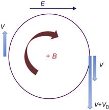
Force F=eE acts across the magnetic field during the one half cyclotron motion in the same direction of rotation, while during the second half it acts in opposite direction. As a result, the test particle will be moving faster from up to bottom and slower from bottom to top.
The difference between these velocities will lead to shift of the cyclotron motion in the direction orthogonal to B and to the force as shown schematically in Figure 4.3. Let us estimate the particle drift velocity taking into account the following acceleration factor as
![]() (4.13)
(4.13)

Thus, during the cyclotron rotation, the particle velocity changes as
![]() (4.14)
(4.14)
Consider Eq. (4.9) for the case in which electric field has only component in x-direction (see Figure 4.3). In this case, transverse components of velocity
![]() (4.15)
(4.15)
![]() (4.16)
(4.16)
After differentiation (assuming the case of constant electric field, Ex=E), one can arrive at
![]() (4.17)
(4.17)
![]() (4.18)
(4.18)
Since both electric and magnetic fields are constant, one can write
![]() (4.19)
(4.19)
Solution for Eqs (4.17) and (4.19) reads
![]() (4.20)
(4.20)
![]() (4.21)
(4.21)
where v⊥ is the velocity in the x–y plane. These equations describe rotation with the frequency ωc and superimposed drift in the negative y-direction, or E×B drift. Drift velocity is the same as it was estimated above (Eq. (4.14)).
The same procedure can be applied for any force transverse to magnetic field, F⊥:
![]() (4.22)
(4.22)
VF is the drift velocity in the case of applied arbitrary force F⊥.
Let us make several general comments regarding the guiding center motion approximation. Strictly speaking this approximation can be used if motion is collisionless as it was assumed in analysis above, i.e., mean free path for collisions is much larger than the characteristic size of the system. In addition, it is assumed that the magnetic field is spatially uniform on the scale of gyroradius:
![]()
4.2 Magnetic mirrors
A configuration of magnetic field used to confine charged particles is called a “magnetic mirror.” Let us consider electron motion in the magnetic mirror as shown schematically in Figure 4.4. A magnetic field having component along z-axis and whose magnitude varies along this axis is considered.

In addition, radial component of the magnetic field has to be taken into account since magnetic field converges. It will be shown that the particle motion in such configuration gives rise to a force. This force can trap the particle in the magnetic mirror.
Assuming the azimuthal symmetry in the cylindrical coordinate system, the equation for the magnetic field (obtained from Maxwell equation) reads
![]() (4.23)
(4.23)
If we assume that (∂Bz/∂z) does not vary with radius, Eq. (4.23) can be integrated:
![]() (4.24)
(4.24)
Therefore, the component of the Lorentz force (Eq. (4.9)) acting on electron in z-direction is
![]() (4.25)
(4.25)
where vθ is the azimuthal velocity. Let us average this force over one gyration consider the guiding center on the axis. In this case, vθ is constant during the gyration and it is equal to v⊥ and r=RL. Thus the average force is equal to
![]() (4.26)
(4.26)
This force pushes the particle into the region of smaller magnetic field (opposite to magnetic field gradient) and it is independent of charge.
Let us define the magnetic moment of gyrating particle as
![]() (4.27)
(4.27)
As the particle moves into the region of a strong magnetic field, its kinetic energy ![]() changes; however, the magnetic moment is conserved as will be shown below.
changes; however, the magnetic moment is conserved as will be shown below.
We start with calculating the total energy of the particle that must be conserved:
![]() (4.28)
(4.28)
where WII is the component of the particle energy in the direction along the magnetic field. The change of the WII is due to force Fz:
![]() (4.29)
(4.29)
where ![]() Using Eq. (4.28), we arrive at
Using Eq. (4.28), we arrive at
![]() (4.30)
(4.30)
Thus,
![]() (4.31)
(4.31)
it follows from Eq. (4.31) that
![]() (4.32)
(4.32)
This means that, the magnetic moment is conserved during the particle motion. The invariance of magnetic moment is the basis for one of the primary approaches for plasma confinement called magnetic mirror. Schematically magnetic mirror device is shown in Figure 4.5.
When charge particle moves from a region of a weak magnetic field to the region of a strong magnetic field, its ![]() should increase in order to keep constant μ. Since total energy of particle remains constant,
should increase in order to keep constant μ. Since total energy of particle remains constant, ![]() must decrease. If the magnetic field in the “bottleneck” of the mirror machine is high enough,
must decrease. If the magnetic field in the “bottleneck” of the mirror machine is high enough, ![]() becomes zero and the particle will be reflected back to the region of a weak magnetic field.
becomes zero and the particle will be reflected back to the region of a weak magnetic field.
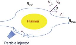
It should be pointed out that the charged particle trapping in the magnetic mirror machine is not perfect. For instance, if the particle does not have velocity component perpendicular to the magnetic field, i.e., ![]() it does not have magnetic moment and force Fz does not act on the particle. A particle with a small v⊥/vII in the region of a weak magnetic field (Bmin) can also escape if the Bmax is not strong enough. Let us estimate the condition for particle trapping. Consider a particle in the region of a weak magnetic field having the total velocity v0 as shown in Figure 4.5. At the turning point vII=0 and magnetic field is Bmax. The invariance of the magnetic moment yields
it does not have magnetic moment and force Fz does not act on the particle. A particle with a small v⊥/vII in the region of a weak magnetic field (Bmin) can also escape if the Bmax is not strong enough. Let us estimate the condition for particle trapping. Consider a particle in the region of a weak magnetic field having the total velocity v0 as shown in Figure 4.5. At the turning point vII=0 and magnetic field is Bmax. The invariance of the magnetic moment yields
![]() (4.33)
(4.33)
It follows from Eq. (4.33) that
![]() (4.34)
(4.34)
where β is the pitch angle in the region of a weak magnetic field. Particles with smaller β will be able to escape and not be trapped in the region of strong magnetic field. In other words, the condition for particle trap is
![]() (4.35)
(4.35)
Equation (4.35) defines the boundary of the region (of a conical shape) in the velocity space or so-called loss cone. Particles lying within the loss cone (i.e., β<βcrit) are not trapped in the mirror. As a result, plasmas in a magnetic mirror machine are not isotropic. It should be pointed out that discussion so far did not include collisions. Due to collisions, particles can be lost after changing their pitch angle and scattering into the loss cone.
4.3 Remarks on particle drift
In the previous sections, we discussed drift of the charged particle in the uniform magnetic and electric fields. It should be pointed out that the presence of any force in addition to the magnetic field could lead to particle drift as it is reflected in Eq. (4.19). Among the typical forces in addition to electric field that affect particle motions are gravity and centrifugal force. Spatial nonuniformity and temporal variation of the magnetic and the electric fields lead to additional drifts.
For instance, presence of the gravity field leads to the following drift:
![]() (4.36)
(4.36)
where g is the gravity constant.
Time-varying electric field leads to the so-called polarization drift:
![]() (4.37)
(4.37)
It should be noted out that in this case, ions and electrons are drifting in opposite directions. In addition, one can see that the drift velocity is proportional to the particle mass and thus the drift velocity of ions will be larger than that of electrons.
As another example, particle motion in the magnetic field having curvature caused centrifugal force leading to the curvature drift:
![]() (4.38)
(4.38)
where Rc is the curvature of the magnetic field.
4.4 The crossed E×B fields plasma dynamics in plasma devices
The devices based on closed electron drift are currently applied in plasma immersion ion implantation, magnetron sputtering, and electric thrusters for spacecraft propulsion. In these devices, theeffect of closed electron drift in a magnetic field is used to maintain large electric field in the quasi-neutral plasma. This electric field is a result of electrostatic coupling of the ion flow and thebackground charge of the closed electron drift. While ion dynamics in most devices can be relatively easily described, the underlying physics of electron transport is not well understood. As it will be shown in Chapter 5, the main problem lies in description of the electron transport mechanism across a magnetic field, which was found to be largely nonclassical. Several possible mechanisms of anomalous electron transport were proposed and investigated over years and some progress was achieved. The related phenomenon of the electric thrusters based on the electron transport in crossed electric and magnetic fields is described in detail in Section 5.2.
One additional example of E×B device is the magnetron, which is an electrical discharge for sputter deposition of thin films [1,2]. Modern magnetrons employ crossed E×B fields that cause a Hall current (Hall drift). It is clear that uncontrolled Hall current will lead to electrons escape from the discharge. Electron losses can be limited by closing the drift current, i.e., by the use of such field configuration that will provide a circular pass of the drift current. In this case, the use of closed-drift configurations ensured a significant increase in the plasma density and sputtering rate.
Recently plasma configurations and electron transport in cylindrical magnetron discharges were studied [3]. It was found that two stable plasma configurations are possible around the negatively biased cylindrical target, namely torus and thin disk. Diffuse plasma torus changes the shape with magnetic field to form a thin disk when the target voltage is less than 400 V. Experiments with low-current magnetrons show that the measured electron mobility across the magnetic field scales as 1/B and not according to classical scaling as 1/B2 [4]. As a result, the concept of anomalous or Bohm diffusion was introduced to describe the electron transport in magnetrons. Recently there was an attempt to analyze the mechanisms of electron cross-field mobility and its impact on the discharge characteristics [5]. The calculated curves for electron energies based on classical and Bohm anomalous diffusion are shown in Figure 4.6. One can see that the classical curve shows too low energy (2 eV versus 4.2 eV or measured/Bohm calculated).
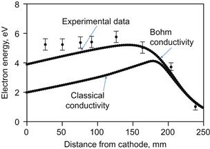
Figure 4.6 Dependence of electron energy on distance from cathode for cylindrical magnetron discharge.
This analysis suggests that the Bohm anomalous diffusion can properly describe the electron transport in cylindrical magnetron. It is interesting to note that in related study of the miniature Hall thruster (that will be discussed in Chapter 5), it was concluded that the Bohm-type diffusion can properly describe the electron cross-field transport [6].
Thus existing experimental evidence and simulations support the idea of the anomalous transport; however, it is not clear what physical phenomena may lead to anomalous electron mobility, and the mechanism of electron transport and plasma turbulence spectra in magnetron plasmas are still an open question.
4.5 Diffusion and transport of plasmas
Understanding the plasma transport phenomena in the presence of gradients of particles and pressure is important for many plasma applications. In this section, we will consider diffusion of plasma in the presence of density gradient. Effect of a magnetic field on the plasma diffusion will also be described.
4.5.1 Basic physics of diffusion
Particle diffusion in a nonuniform plasma arises due to friction term. We start with the steady-state momentum equation:
![]() (4.39)
(4.39)
where vcoll is the total momentum transfer frequency. Further analysis will be performed using the following basic assumptions:
Solving Eq. (4.39) for velocity v, we obtain
![]() (4.40)
(4.40)
By introducing the flux Γ=nv, Eq. (4.40) can be rewritten as
![]() (4.41)
(4.41)
Let us introduce two new parameters:
![]() (4.43)
(4.43)
With these coefficients, one can write the equation for flux (Eq. (4.41)) as
![]() (4.44)
(4.44)
In this equation, positive sign corresponds to ions and negative to electrons. The process of diffusion in the absence of the electric field is called free diffusion:
![]() (4.45)
(4.45)
Equation (4.45) is called Fick’s law. Substituting this equation into the continuity equation ((∂n/∂t)+∇·(nv)=0) without the source and sink terms, one obtains
![]() (4.46)
(4.46)
Note: It should be pointed out that mobility and diffusion coefficients (or transport coefficients) are related by the so-called Einstein relations:
![]() (4.47)
(4.47)
4.5.2 Ambipolar diffusion
In this section we will consider diffusion of plasma, i.e., coupled diffusion of ions and electrons. Typically flux of electrons is initially much larger than that of ions so that electric field will be build up to maintain zero total charge flux. Such diffusion process of electrons and ions without charge buildup will be called ambipolar diffusion. In the following analysis, plasma quasi-neutrally is assumed. Thus the basic conditions to be considered are
![]() (4.48)
(4.48)
![]() (4.49)
(4.49)
From Eq. (4.48), we obtain that
![]() (4.50)
(4.50)
Solving this equation for electric field yields
![]() (4.51)
(4.51)
Equation (4.51) can now be substituted into diffusion equation for ions:
![]() (4.52)
(4.52)
This equation has a form of the Fick’s law (Γ=−Da∇n) if we introduce a new coefficient that will be called ambipolar diffusion coefficient:
![]() (4.53)
(4.53)
Typically in plasma discharges, the electron mobility is much higher than that of ion mobility (i.e., μe![]() μi) and thus expression for ambipolar coefficient can be simplified:
μi) and thus expression for ambipolar coefficient can be simplified:
![]() (4.54)
(4.54)
One can see that diffusion is tied to the slower species (ions in this case). Using the Einstein relation, one can obtain that
![]() (4.55)
(4.55)
Thus one can see that ambipolar coefficient is proportional to the electron temperature, so that at higher electron temperature, ions and electrons will diffuse at the greater rate that in the case of ion diffusion rate.
4.5.3 Diffusion across a magnetic field
In this section we will discuss effect of the magnetic field on the plasma diffusion. Collision can change particle gyration around the magnetic field. On average collision moves the center of gyration by the Larmor radius. Since such process is random, it is similar to diffusion. In this case the Larmor radius can replace the mean free path for collisions.
In order to derive the diffusion coefficient across the magnetic field, we start with transverse component of the momentum equation:
![]() (4.56)
(4.56)
Schematically the process of diffusion is shown in Figure 4.7. Consider component of Eq. (4.56) in x-direction for electrons:
![]() (4.57)
(4.57)
![]() (4.58)
(4.58)
if we use definitions of mobility and diffusion coefficient, these equations can be rewritten as
![]() (4.59)
(4.59)
![]() (4.60)
(4.60)

Let us introduce the ratio of the cyclotron frequency to the collisional frequency i.e., β:
![]()
By substituting expressions for velocities vx and vy, Eqs (4.59) and (4.60) can be solved simultaneously for vx and vy:
![]() (4.61)
(4.61)
![]() (4.62)
(4.62)
One can introduce transport coefficients across the magnetic field:
![]() (4.63a)
(4.63a)
![]() (4.63b)
(4.63b)
It should be pointed out that Hall parameter β is an important parameter that indicates the degree of plasma confinement in a magnetic field. In the case of β2![]() 1, the diffusion coefficient across the magnetic field reduces to
1, the diffusion coefficient across the magnetic field reduces to
![]() (4.64)
(4.64)
Diffusion of electrons across a magnetic field is much smaller than that of ions due to electron magnetization:
![]()
If plasma flows across the magnetic field, one can introduce the ambipolar diffusion similarly to Eq. (4.54) except the transport coefficients across the magnetic field should be described as follows:
![]() (4.65)
(4.65)
In the magnetic field, the mobility of ions is higher than that of electrons, thus diffusion coefficient across the magnetic field can be approximated as
![]() (4.66)
(4.66)
Recall that the ambipolar diffusion coefficient is determined by the slower species (similarly to the case without a magnetic field), which is the one for electrons in the case across a magnetic field.
Plasmas (and in particular plasmas in a magnetic field) are subject to various instabilities as it was described in Chapter 1. Instabilities tend to destroy magnetic confinement due to development of a larger-amplitude turbulent diffusion. The diffusion has the upper limit of the Bohm diffusion that can be described by coefficient [7]:
![]()
The scaling of the Bohm diffusion coefficient as 1/B (compare to classical diffusion scaling as 1/B2, see Eq. (4.64)) makes it very important transport mechanism across the magnetic field as it will be described in Chapter 5.
4.6 Simulation approaches
In this section we will describe basic approaches for plasma modeling and, in particular, approaches that are based on numerical simulations. Two basic approaches were developed in plasma physics and engineering. First one is based on the fluid description of plasma solving numerically magnetohydrodynamic (MHD) equations. Such approaches capture flow field characteristics, however, lacking the ability to calculate the transport coefficients. The second one is the kinetic model particle techniques that take into account kinetic interactions among particles and electromagnetic fields. This simulation is computationally extensive as it is able to resolve local parameters of the plasma. By taking advantages of both simulation approaches, there are hybrid approaches with various levels of kinetic and fluid combinations. All these simulation approaches have their specific advantages and limitations that will be illustrated in this section.
More rigidly the difference between the fluid and kinetic approaches can be illustrated as follows: fluid approach treats the large-scale properties of plasma involving mass, momentum, and energy transport, while the kinetic approach provides accurate treatment of local processes (collisions, scattering) and transport properties.
We will start with description of the kinetic analysis.
4.7 Particle-in-cell techniques
Basic for analytic treatment of the plasma kinetics is the Vlasov equation:
![]() (4.67)
(4.67)
where f(x,v,t) is the distribution function, v is the velocity, E is the electric field, and B is the magnetic field.
Note: The Vlasov equation treats the collisionless plasma condition. If collisions between particles are important, one needs to consider a model for Boltzmann equation with the collisional term (collision integral) that will appear in the right-hand side of Eq. (4.67).
Common approach to kinetic modeling is to represent f(x,v,t) by a number of macroparticles (MPs) and compute the particle orbits in a self-consistent E and B. This is equivalent to solving the Vlasov equation by the method of characteristics.
Dawson [8] treated particles as discrete points and computed electric field force assuming explicitly the Coulomb interactions with each other particle. Number of pairs is N(N−1)/2~N2, where N is the number of particles.
Note: Consider 107 particle, 104 time steps and assume that in order to evaluate the force, we need 10 operations. The total number is N(N−1)/2×104×10~5×1018. If each operation will take 10−9 s, the total time will be 109 s.
Another approach is to use the spatial grid. In this case particles and current densities can be calculated using the interpolation scheme. Fields are solved on the grid while forces are interpolated. This procedure is called particle-in-cell (PIC) method. Number of operation per time step are reduced to N log(N).
PIC is a technique commonly used to simulate the motion of charged particles or plasma. The calculation flow chart in PIC is shown in Figure 4.8.

For each time step, the equation for the field is solved and the particle motion is implemented.
At t=0 initial conditions are given and particle velocity and positions are prescribed. Particles are loaded with each particle having index (Vi, Xi). Transition from particles to quantities (charge density, current) is made by calculating the charge and current density on the grid. This procedure is called weighting from the grid points and it depends on particle position. After charge density is calculated the electric field can be computed. Similarly once the current is calculated, the self-magnetic field can be computed as well. By calculating the electric field, we interpolate the fields from the grid to particle in order to apply force at the particle by performing again weighting. The following information for each particle is stored in the computer memory: (Vi, Xi, qi, mi). Usually there are more particles than the grid points.
Charged particles interact with each other by attracting particles of opposite charge and repelling those with the same charge. This is represented by the Coulomb force and is given by
![]() (4.68)
(4.68)
where q1,q2 are charges and r is the distance between interacting particles.
In principle, taking a collection of particles representing the real physical ions and electrons and directly computing this force can simulate plasmas. However, plasma simulations generally require at least 1 million particles in order to reduce numerical errors. Since Coulomb force leads to an n2 problem, computation of a single time step would require at least 1 trillion operations.
Note: In the following, we describe the procedure for PIC simulation following the time chart as shown in Figure 4.8. We will start with integration of the equation of motion.
4.7.1 Equation of motion
In general we have many particles and many time steps, so the method for calculating particle trajectories and electric field should be as fast as possible but should retain some accuracy. Also we want to store the minimum amount of information (not to have previous time steps Vi and Xi for high-order integration). Commonly used integration method is the leapfrog method. It is fast and numerically stable. First, we integrate velocity through the time step. Next, position is updated. The name comes from the fact that times at which velocity and positions are offset from each other by half a time step. As such, the two quantities leap over each other. This idea is shown in Figure 4.9.

Figure 4.9 The leapfrog method. In this approach velocity and positions are offset from each other by half a time step.
The equations that must be solved are
![]() (4.69)
(4.69)
![]() (4.70)
(4.70)
where F is the force. Finite-difference representation for these equations is
![]() (4.71)
(4.71)
![]() (4.72)
(4.72)
Positions are given at t=0, while velocities are at t−Δt using transformation employing force F(t=0). If we need to resolve oscillations or waves, we need to preserve
![]() (4.73)
(4.73)
where ωp is the plasma frequency. If magnetic field is used, the rotation of particle using the following equation should be performed:
![]() (4.74)
(4.74)
After particles are moved to new positions, it is necessary to verify that all particles are still in the computational domain. To this end boundary conditions should be examined. Two boundary interactions are possible. The particles can either exit the domain or collide with solid objects. Computational boundaries are either open (or absorbing, allowing particles to leave), reflective (elastically returning particles into the domain), or periodic (particles are transported to the opposite side of the domain). The reflective boundary is used to identify planes of symmetry.
4.7.2 Integration of the field equations
At this point, charges (ρ) and current densities (J) are assigned to the grid points, so we can calculate E,B using the Maxwell’s equations as sources. For instance, electric field can be calculated as
![]() (4.75)
(4.75)
Here ρ is the charge density. Electric potential is computed from E=−∇φ. Electric potential can be directly computed from the Poisson equation:
![]() (4.76)
(4.76)
Here ε0 is the permittivity of free space. Charge density is calculated as
![]() (4.77)
(4.77)
The subscripts i and e denote ions and electrons, respectively, and Zi is the average ion charge number.
Note: Due to very large mass ratio between ions and electrons, there is large difference in the characteristics times for ion and electron motion. Typically in order to resolve the electron motion, one needs to employ extremely small computation time steps (around 10−12 s). In other words, in the frame of reference of the ions, electrons move instantaneously. Therefore, if resolving electron motion is not essential for the particular problem of interest, it is possible to simplify the analysis by considering electrons as a fluid.
In this case, the electron density is then given by the Boltzmann relationship
![]() (4.78)
(4.78)
where n is the reference density and φ0 is the reference potential.
4.7.3 Particle and force weighting
The following procedure should be conducted to calculate the charge density and forces in the cell:
Calculate charge density on the discrete grid points taking into account particle positions.
Calculate the force on particles from fields on grid points.
This procedure is called weighting (form of interpolation). It is desirable to have the same weighting in both density and force to avoid a self-force (i.e., particle moves by itself).
4.7.3.1 Zero-order weighting
We need to count the number of particles within ±(Δx/2) which is the cell width about the jth grid point (Figure 4.10):
![]() (4.79)
(4.79)
where N(j) is the number of particles.

In this case, the computation is fast with only the one grid lookup. The same force F will be applied for all particles in jth cell. If particle moves into jth cell, density will increase, while if particle moves out of the cell the density will decrease. As a result, motion of the particle in and out of the cell will produce the noise.
4.7.3.2 First-order weighting
The idea is to smooth out the density and field fluctuations (noise). However, in this case, we need to use two grid points for each particle. This is more computationally expansive but produces better interpolation.
Particles are finite size rigid clouds that can freely pass through each other (the idea was proposed by Birdsall in 1969, called clouds in cells (CIC)) [9].
Let the total cloud charge be qC. The charge that the particle carries and that is assigned to j is
![]() (4.80)
(4.80)
Part of the charge that is assigned to j+1 is
![]() (4.81)
(4.81)
The net effect is to produce a triangular particle shape S(x) which has width 2Δx. Assignment to nearest grid point is called PIC [9]. As a particle moves through the grid, it contributes to density much more smoothly than the zero-order weight.
The field or force weight is similar. The first-order force comes from linear interpolation:
![]() (4.82)
(4.82)
4.7.4 Particle generation
In PIC, new particles are generated by sampling sources. Particle generation depends on specifics of the type of particle generation. For instance, particles can be generated at the electrode surface to model emission, or at the spacecraft thruster exit plane to model charge particle ejection. In some instances, all particles will be loaded initially, and the simulation will only compute their final distribution state. In many case of practical interest, particles are generated with the Maxwellian distribution. According to Birdsall and Langdon [9], the Maxwellian distribution can be approximated as
 (4.83)
where M is some number and Ri is an ith random number in range [0:1). The value chosen for M controls the accuracy of this method. It was suggested to use M=12 to prevent entries larger than six times the thermal velocity.
It should be pointed out that often the following simplification can be made. The current carried by the plasma can be assumed to be low and as a result the self-induced magnetic field can be neglected. If no external magnetic field is applied, the set of underlying Maxwell’s equations is reduced. This is the electrostatic PIC code.
An approach called particle-in-cell–Monte Carlo collisions (PIC-MCC) simulations is widely used to simulate very low-pressure plasmas taking into account rarefied collisions. In this approach the collisions such as ionization, excitation, momentum, and charge exchange between particles are treated with random numbers.
4.7.5 Example of application of PIC simulations
As an example, we consider a case of the plasma flow along the wall leading to formation of the interface-sheath between the plasma and the wall. Let us consider the sheath formation in the presence of a two-dimensional (2D) magnetic field incident to the wall. The analysis is performed using a 2D PIC code. For this example, a simple axisymmetric electrostatic particle-in-cell (ES-PIC) code was used. The code is based on the hybrid approach in which ions are treated as particles, but electrons are represented by a fluid model. As illustrated in Figure 4.11, the computational domain is limited to a small region near the wall. The small size of the domain allows resolving the Debye length and thus directly computes the electric potential in a reasonable amount of time (each simulation takes approximately 20 min). The upper boundary represents the outer wall, while the bottom boundary extends into the quasi-neutral bulk plasma region. Ions are injected into the simulation along the left boundary and leave through the open right and bottom face or by recombining with the upper wall.

Figure 4.11 Schematics of the computational domain. Ion particles are injected from the left. Poisson equation with Boltzmann electrons is used to compute electric potential. Reference potential and density for the Boltzmann relationship vary with the magnetic field line. Source: Reprinted with permission from Ref. [39]. Copyright (2012) by American Institute of Physics.
To simplify the subsequent computation, we select a simulation mesh in which the radial gridlines are aligned with the magnetic field. Such a formulation allows us to specify the necessary reference values as a function of the axial grid coordinate only. An example of the simulation is shown in Figure 4.12. Plasma density distribution along the flow and the wall is shown. Plasma density decreases due to acceleration along the flow direction as well toward the wall. Ion densities are shown using the contour plot. Velocity streamlines as well as the sheath boundary are also plotted. The sheath edge is plotted by the solid red line and corresponds to the contour where the radial velocity component (i.e., the component normal to the wall) reaches the Bohm velocity. The sheath forms a short distance from the injection plane and continues to grow as more ions are accelerated from the bulk plasma toward the wall. Plasma density decrease is also influenced by the net increase in ion velocity due to the axial electric field.
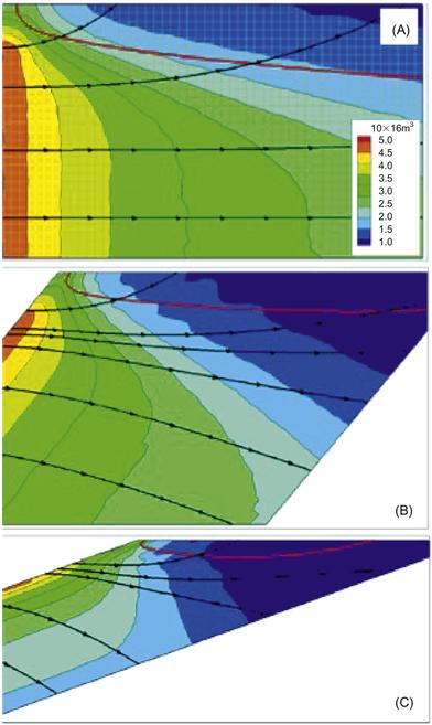
Figure 4.12 Simulation results showing the ion density profile for three different magnetic field line angles, 0° (A), 40° (B), and 70° (C), respectively. Streamlines show ion trajectories. The red lines correspond to the sheath edge as computed with the Poisson solver. The sheath edge is plotted by the solid red line and corresponds to the contour where the ion velocity component normal to the wall reaches the Bohm velocity. Source: Reprinted with permission from Ref. [39]. Copyright (2012) by American Institute of Physics.
The particle-in-cell code is available as a supplemental material to this book and it was provided by Particle-in-Cell Consulting Inc www.particleincellconsulting.com (Dr. Lubos Brieda).
4.8 Fluid simulations of plasmas: free boundary expansion
In this chapter, we consider fluid simulation of plasmas. In particular, an example of plasma jet expansion will be described. This example will be illustrated on the specific case of the free boundary plasma jet expansion from the cathode spot of the vacuum arc.
4.8.1 Fluid model of vacuum arc plasma jet
A general model for the plasma jet expansion, in particular, plasma jet from the cathode spots of a cathodic arc, should consider the changes in the plasma parameters at distances sufficiently large where plasma density is much lower than that in the region near to the spots.
The theoretical study of vacuum arc plasma jets has been concentrated on the plasma jet formation and magnetic collimation effects. Beilis et al. [10,11] and Hantzsche [12] studied the plasma jet without the presence of an axial magnetic field (AMF) for the various plasma density regions. It may be noted that in the low-density part of the plasma jet, an AMF may have a very significant effect on the jet expansion. 2D free jet plasma expansion in an AMF was analyzed and simulated by Keidar et al. [13]. The problem of the 2D free plasma jet expansion is very complicated and a numerical method is needed in order to obtain the solution in the general case. One of the main difficulties in the jet expansion problem is the formulation of the physical conditions at the plasma–vacuum boundary.
The free boundary conditions at the interface between the plasma and the vacuum in the case of large current density, where the self-magnetic field plays a significant role, were discussed by Huysmans et al. [14]. The plasma boundary was defined by the condition that the magnetic field lines cannot point out of the plasma (i.e., the normal component of the magnetic field at the plasma boundary must be equal to zero). The jump in the tangential component of the magnetic field across the boundary is defined as the surface current. The boundary condition that the normal component of the plasma velocity to the fixed plasma boundary must be zero was also used by Kress and Riedel [15,16].
4.8.2 Basic model
Let us discuss the plasma jet with characteristic radius Ro (Figure 4.13) at some distance from the cathode surface where the jets from the individual cathode spots in the case of the multicathode-spot vacuum arc are averaged and therefore all plasma parameters will be assumed to be uniform. This plasma is sufficiently rarefied so that inelastic collisions (ionization, recombination, etc.) do not cause changes in the plasma density. In addition, it is considered that the electron and ion temperatures are different but do not change substantially during expansion. In these conditions, the electric field in the interelectrode gap does not significantly influence the expansion of the plasma jet but may play a dominant role in the current collection at the anode.
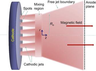
The anode is assumed not to influence the flow field and only acts as a current collector. The imposed AMF has only an axial component. The geometric position of the free boundary will be determined as part of a self-consistent solution.
The steady-state plasma flow in the vacuum arc is characterized by a directed velocity V of about 104 m/s, which is larger than the thermal velocity. The plasma jet of the low-current vacuum arc (IARC~100–300 A) has a plasma density in the rarefied part of the cathode region [10,11] of about 1020 m−3 and a characteristic radius of about few cm. Taking into account that the electron temperature (Te) is about 1–2 eV, we have a mean free path Lc, which is 10−3 m. The magnetic diffusion time τ is about 10−7 s. This problem is characterized by a timescale of τf=L/V, where L is the interelectrode region length. For L~0.1 m, τf is about 10−5 s.
The current carrying plasma flow in the magnetic field will be studied with the aid of the following assumptions based on the above estimations:
1. The plasma is fully ionized and consists of two species of charged particles.
2. During the expansion, the temperature of each species is not substantially changed and thus can be considered constant.
3. The plasma parameters at the starting plane and in most of the expansion region having a characteristic length L is such that the mean free path for electron–ion collisions (Lc) is much smaller than the L. Thus, the hydrodynamic approximation may be used to describe the flow of the plasma in the magnetic field.
4. The electron component is not inertial and thus (me(Ve·∇)Ve≈0).
5. Quasi-neutral plasma expansion is considered, i.e., |Ne−ZiNi|/Ne![]() 1, where Ne and Ni are the electron and ion densities, respectively, and Zi is the ionicity.
1, where Ne and Ni are the electron and ion densities, respectively, and Zi is the ionicity.
The behavior of this steady-state plasma may be described by the momentum conservation equations:
![]() (4.84)
(4.84)
![]() (4.85)
(4.85)
and the mass conservation equations:
![]() (4.86)
(4.86)
![]() (4.87)
(4.87)
where Vi and Ve are ion and electron velocities, respectively, mi and me are the ion and electron masses, respectively, m*=mime/(mi+me)≅me is the effective mass. P is the partial pressure, E is the electric field, νei is the electron–ion collision frequency:
![]()
where Te is the electron temperature (in eV) and ln Λ is the Coulomb logarithm. In addition, we use the definition νeiNe=νieNi.
Let us define the electric current density j=eN(Vi−Ve) and the plasma conductivity σ=(e2N/meνei). The ions and electrons are assumed to be ideal gases with partial pressures Pα=eTαNα, where α=e, i, and k is Boltzmann’s constant. By using the last expressions and condition, N=Ne=ZiNi, and adding Eq. (4.84) with Eqs (4.85) and (4.86) with Eq. (4.87), Eq. (4.84) may be written in the following form:
![]() (4.88)
(4.88)
![]() (4.89)
(4.89)
![]() (4.90)
(4.90)
![]() (4.91)
(4.91)
Let us discuss the situation in which the plasma parameters are such that the electrons are magnetized, while the ions are not, i.e., where ρi![]() L
L![]() ρe, where ρe, ρi are the electron and ion Larmor radii, respectively. Equations (4.88)–(4.91) may be written in component form in cylindrical coordinates (see Figure 4.13) by taking into account that the magnetic field has only an axial component (i.e., B=izBZ):
ρe, where ρe, ρi are the electron and ion Larmor radii, respectively. Equations (4.88)–(4.91) may be written in component form in cylindrical coordinates (see Figure 4.13) by taking into account that the magnetic field has only an axial component (i.e., B=izBZ):
![]() (4.92)
(4.92)
![]() (4.93)
(4.93)
![]() (4.94)
(4.94)
![]() (4.95)
(4.95)
![]() (4.96)
(4.96)
![]() (4.97)
(4.97)
where Vz and Vr are the axial and radial components of the ion velocity, respectively, jr, jz, jθ are radial, axial, and azimuthal components of the current density, respectively, Cs2=k(ZiTe+Ti)/mi, βe=ωe/νei, where ωe=eB/me. In the momentum conservation equation for ions, the term with magnetic field is absent as a result of the ion being unmagnetized.
Let us use Eqs (4.94)–(4.97) in order to express the equation for the electric field in explicit form. Taking into account that the Coulomb logarithm ln Λ has a weak dependence on the density N, we obtain that νei=a·N, where a=constant. After some linear transformations in the expressions for ∂jr/∂r and ∂jz/∂z, and using the definition E=−∇φ, we obtain the following expression for the potential distribution φ:
 (4.98)
The boundary conditions for this system of equations will be discussed below for free plasma jet expansion.
4.8.3 Free plasma jet expansion
In this section, the current carrying plasma flow in the magnetic field is analyzed using the free jet expansion approach. We assume that the arc runs to an annular or ring anode, and that the characteristic size of the cathodic plasma (e.g., the cathode radius or the cathode-spot radius) is smaller than the inner radius of the anode and thus a free jet flow occurs.
4.8.4 Boundary condition for free plasma jet expansion
Mathematically, the free boundary problem consists of a system of partial differential equations, together with the necessary boundary conditions. The free boundary is unknown and must be determined as part of the solution. General approach for the solution of the free boundary problem is the trial free boundary method.
Generally, in order to solve the system of equations (4.92)–(4.98), it is necessary to know the geometric position of the plasma boundary, where two kinds of the boundary conditions, (1) hydrodynamic conditions for the plasma density and velocity, and (2) electrostatic conditions for the electric potential and electric field, are required.
If the plasma is in a stable steady state, the shape of the boundary is described by a function α(z), which is the angle of the jet boundary (Figure 4.14).

The main problem then is to develop an equation for this function. Let us introduce the spatial coordinate in the direction n normal to the boundary and the coordinate τ in the direction tangential to the boundary. The plasma velocity direction is tangential to the boundary and therefore the normal component Vn is equal to zero (point A in Figure 4.14). At the point C, the normal n1 and tangential τ1 vectors are translated and rotated relative to the normal and tangential vectors at point A. The angle between the tangential axis τ1 and the old axis τ at C is equal to the jet angle change from point A to point C. According to Figure 4.14, the jet angle change from the point A to the point C in the limit of very small distances between points A and C may be defined as α(C)−α(A)=tan−1(Vn/Vτ), where α(A) is the jet angle at point A, α(C) is the jet angle at C, and Vn and Vτ are the normal and tangential components of the velocity vector at C in the coordinate system {n,τ}. The change in the jet angle α can be obtained by differentiation of the above expression:
![]() (4.99)
(4.99)
The velocity component Vn changes along axis τ from zero at the point A to some nonzero value. Taking into account that (∂Vn/∂τ)≠0 and Vn=0 at point A, together with Eq. (4.99), yields the final expression for the jet angle change at point A:
![]() (4.100)
(4.100)
In order to solve this equation, an expression for ∂Vn/∂τ and Vτ will be obtained from the n-components of Eq. (4.92) (see Figure 4.14):
![]() (4.101)
(4.101)
where the normal component of the vector j×B is given [j×B]n=jθB cos(α) and α is the jet angle. Taking into account that Vn=0 at the boundary and using Eq. (4.100), we have the following simplified form of Eq. (4.101):
![]() (4.102)
(4.102)
where ωi=eB/mi. Vτ is obtained from the tangential component of Eq. (4.88) using the boundary condition Vn=0:
![]() (4.103)
(4.103)
The velocity components will be obtained from Eqs (4.102) and (4.103) assuming that the plasma density and current distribution are known (a specific boundary condition will be discussed below), and the jet angle change will be calculated.
The generalized equation for the velocities will now be obtained in order to investigate the influence of the boundary conditions. We can solve Eq. (4.102) for jr and then substitute this expression into Eq. (4.103), we obtain the following expression:
![]() (4.104)
(4.104)
The main theoretical problem in the plasma expansion is defining the boundary conditions for the density and electric potential at the plasma–vacuum interface. The condition for the density on the external surface of the boundary layer is N=0 in the case of plasma expansion into vacuum, as illustrated in Figure 4.14.
In order to close the problem of the free boundary jet expansion, the boundary conditions for the potential will be formulated. The present model is based on the premise that the current carrying plasma flows from the cathode to the anode, which does not influence the flow field. At the anode plane, we set the anode potential, which is the boundary condition for the potential equation (see Eq. (4.98)). This procedure models the physical conditions presented by a grid anode, and to some extent those presented by a large diameter thin ring anode. At the free plasma boundary, the condition Jn=0 is used and then we have following equation for the electric field at the plasma boundary:
![]() (4.105)
(4.105)
Let us discuss two limiting cases for the above equation. When B=0, it reduces to the simple equation in which the electrical field at the plasma boundary depends on the electron temperature and density gradient. In the general case (B≠0), the component of the electric field normal to the plasma boundary is dependent on the magnetic field and for large magnetic fields may change sign, and in the limiting case when ∂N/∂n=0, it will be determined by the magnetic field and current density.
The system of equations (4.92)–(4.105) with boundary conditions for the density, potential, and current fully determines the free boundary jet expansion problem. The ion velocity, current density, and density distribution are obtained numerically using the implicit second-order accuracy method [17].
4.8.4.1 Example of calculation of free boundary plasma jet expansion
The model that will be described here is related to the single or multicathode-spot vacuum arc plasma jet expansion. The problem was analyzed using dimensionless variables, where all velocities are normalized by Cs, the density by density at the starting boundary No, all coordinates by Ro, electrical current density by eNoCs, and the electrical potential by the electron temperature (kTe/e). In this example, plasma parameters were chosen to correspond to the Ti plasma jet.
The calculated plasma jet boundary in the r–z plane is shown in Figure 4.15 for different magnetic fields for the following conditions: arc current I=200 A, initial Mach number M=5, electron temperature Te=2 eV [10,11], Ti/Te=0.5, Zi=1, ion current fraction fi=0.1, plasma density at the starting plane No=1020 m−3, which corresponds to the conditions in the external part of the cathode jet.

Figure 4.15 The plasma free jet boundary in the r–z plane with magnetic field as the parameter. Initial Mach number M=5. Ion temperature to the electron temperature ratio Ti/Te=0.5, electron temperature Te=2 eV, arc current I=200 A, initial plasma density No=1020 m−3, ion current fraction fi=0.1. Source: Reprinted with permission from Ref. [13]. Copyright (1996) by Institute of Physics.
The jet has an approximately conical shape with an angle which changes in the axial direction and depends on the magnetic field. The main jet shape changes occur over axial distances z~(3–4)Ro. The jet angle and the plasma density decrease did not change substantially at the larger distances z>4Ro. The potential drop U between (r,z)=(0,0) and (0,4Ro) depends on the electron temperature and in the case of Te=2 eV it was found that U=8.4 V for B=0 and U=9 V for B=0.01 T at z=4Ro. The electric equipotential surfaces were normal to the z-axis (i.e., Er is small) except near the boundary as shown in Figure 4.16.

The normalized axial current density distribution Jz(r) for different distances from the initial plane and magnetic fields is shown in Figure 4.17, and the radial current density distribution Jr(r) is plotted in Figure 4.18. The radial current density component has its maximum value off-axis, while the maximum Jz(r) is on the axis. This off-axis maximum in Jr(r) is caused by the strong plasma density changes in the region of maximum.
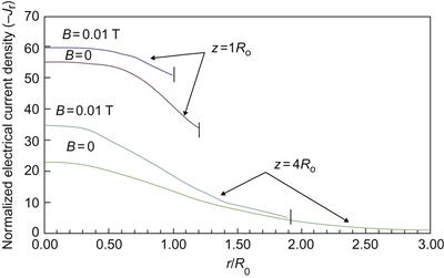
Figure 4.17 Normalized axial electrical current density distribution for magnetic fields B=0.01 T and B=0. I marks the plasma boundary. Source: Reprinted with permission from Ref. [13]. Copyright (1996) by Institute of Physics.

Figure 4.18 Normalized radial electrical current density distribution for the magnetic field B=0.01 T and B=0. I marks the plasma boundary. Source: Reprinted with permission from Ref. [13]. Copyright (1996) by Institute of Physics.
The normalized radial plasma density distribution for z=4Ro with the magnetic field as parameter is presented in Figure 4.19. For the relatively large magnetic fields of B>0.01 T, the plasma density distribution near the boundary asymptotically approaches the condition of the radial density gradient equaling zero.

Figure 4.19 Normalized radial density distribution with magnetic field as a parameter. I marks the plasma boundary position. Source: Reprinted with permission from Ref. [13]. Copyright (1996) by Institute of Physics.
The plasma density distribution for different distances from the initial plane in the case of a 0.01 T magnetic field is plotted in Figure 4.20. The radial plasma density gradient in the boundary region is seen to approach zero with z>3Ro.

Figure 4.20 Normalized radial density distribution for different distances from the initial plane. I marks the plasma boundary position. Source: Reprinted with permission from Ref. [13]. Copyright (1996) by Institute of Physics.
The conditions for plasma collimation depend on the initial plasma density at the starting plane. If the plasma density at the starting plane is known, then it is possible to obtain good collimation (jet angle less than 20°) by the proper choice of magnetic field.
The radial distribution of the axial and radial velocity components at z=4Ro are presented in Figure 4.21 for initial Mach number M=5 with magnetic fields of 0.001 and 0.01 T. The axial velocity in both cases slightly increases due to the pressure gradient. The radial velocity increases approximately linearly starting from zero on the axis and reaching significant values at the plasma boundary as a result of the expansion into the vacuum. In the 0.001 T case, the magnitude of the radial velocity approaches the axial velocity.

Figure 4.21 The radial distribution of the axial and radial velocity components at z=4Ro with the magnetic field as parameter. I marks the plasma boundary position. Source: Reprinted with permission from Ref. [13]. Copyright (1996) by Institute of Physics.
The presence of a stronger magnetic field, however, restricts the axial growth of the radial velocity, as can be seen in Figure 4.22, where the radial to axial velocity ratio at the plasma boundary is shown. Based on this results one can conclude that the streamline angle is about 40° for the 0.001 T magnetic field and about 20° for 0.01 T.

Figure 4.22 A plot of the radial to the axial velocity ratio at the plasma boundary with magnetic field as the parameter. Source: Reprinted with permission from Ref. [13]. Copyright (1996) by Institute of Physics.
The normal component of the electric field at the plasma boundary is shown in Figure 4.23. In the case of βeo→0 at the starting plane, a space charge layer is formed at the plasma–vacuum transition, in which the potential drop depends on the electron temperature and plasma density gradient. In the more general case with the presence of a magnetic field (values at the starting plane of βeo=0.01 or βeo=0.5 in Figure 4.23), this layer is also present, but at some point in the jet expansion where βe≥1 the electric field changes sign. This occurs because the electrons are strongly magnetized while the ions are unmagnetized, and thus the electrons are confined and produce an electric field with a polarity that retards ion flow from the plasma. This electric field perturbs the plasma neutrality at the plasma boundary.

Figure 4.23 The distribution of the normal component of the electric field at the plasma boundary with βeo at the starting plane (z=0) as parameter. Source: Reprinted with permission from Ref. [13]. Copyright (1996) by Institute of Physics.
The normal component of the electric field at the plasma boundary decreases with axial distance. This is caused by decrease in the plasma density gradient.
4.8.4.2 Example of calculation: hollow anode vacuum arc
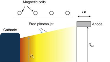
It is follows from Section 4.8.4.1 that in order to control the plasma jet parameters far from the cathode spot and to collimate the plasma flux from the plasma source, it is necessary to apply an AMF. Magnetic collimation of the plasma jet is limited by the growth of arc voltage, and the arc becomes increasingly unstable with increasing of the magnetic field component perpendicular to the cathode–anode direction. To this end, in this example, we analyze electrical characteristics such as current collection on the anode and voltage distribution in the interelectrode gap of the vacuum arc with a hollow anode. The problem is shown schematically in Figure 4.24.
Let us focus now on the boundary conditions at the plasma-near anode region interface.
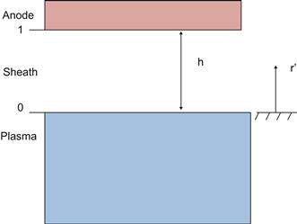
4.8.4.2.1 Near anode region (anode sheath)
The plasma–anode interface consists of a sheath with charge separation. A 1D sheath will be considered because generally the sheath thickness (~LD) is smaller than the anode length La (Figure 4.25). Let us assume that the electrical current in the sheath is carried mainly by electrons, i.e., Ji/Je![]() 1. The electrons are magnetized in the sheath and drift in the direction parallel to the wall. The electron current in the direction toward the wall is the result of electron collisions even when the collision mean free path is smaller than the sheath thickness. Taking into account strong electron magnetization (βe
1. The electrons are magnetized in the sheath and drift in the direction parallel to the wall. The electron current in the direction toward the wall is the result of electron collisions even when the collision mean free path is smaller than the sheath thickness. Taking into account strong electron magnetization (βe![]() 1), and after neglecting the pressure gradient force in Eq. (4.89) the following expression for the electron velocity can be obtained:
1), and after neglecting the pressure gradient force in Eq. (4.89) the following expression for the electron velocity can be obtained:
![]() (4.106)
(4.106)
In the sheath (where generally Ne≠ZiNi), the equation system (4.92)–(4.97) will be supplemented by Poisson’s equation:
![]() (4.107)
(4.107)
The solution of Poisson’s equation (Eq. (4.107)) for the potential distribution under the above conditions, after taking into account Eq. (4.106), has the following form [40]:
![]() (4.108)
(4.108)
![]()
where Jer is the radial current density on the anode, φo and (∂φ/∂r)o are the potential and the potential gradient at the plasma–sheath boundary, respectively (Figure 4.25, boundary 0).
Taking into account that the thickness of the space charge sheath approximately equal to the Debye length, it is possible to obtain the dependence of the anode sheath drop Ush as a function of the magnetic field. The total arc voltage U (excluding the cathode voltage drop) consists of the voltage drops in the quasi-neutral plasma Upl and sheath voltage drop Ush. The voltage in the plasma Upl depends on the electrical current distribution j(r,z) which is obtained from the 2D calculation of free jet expansion.
The calculated jet voltage Upl in the plasma and the sheath voltage drop Ush are shown in Figure 4.26. The jet voltage Upl was calculated in the quasi-neutral plasma for fixed arc current and interelectrode gap geometry. The sheath voltage drop was calculated using the definition Ush=φ(h)−φ(0).

Figure 4.26 Voltage drop as a function of magnetic field. Ti, I=200 A, Te=2 eV, Ti/Te=0.5, z=0.5Ro, Ran/Ro=1, r=0.5.
The voltage drop decreases with anode length La as shown in Figure 4.27, where γ=La/Ro. The calculated results were compared with experiments with different anode length to the cathode radius ratio γ and were plotted in Figure 4.28. Note that in experiment, cathode radius Rc was used as a characteristics scale of the plasma jet radius.

Figure 4.27 Total voltage drop U as a function of magnetic field with γ as parameter. z=0.5Ro, Ran/Ro=1.

Figure 4.28 Voltage drop as a function of magnetic field, experiment, and theory for different γ: (a) (γ=1) [18], (b) (γ=10) [19], and (c) (γ=0.4) [20].
Experimental parameters and assumptions taken into account in this calculation are given in Table 4.1. In both the experiments and theory, larger voltage drops are observed with smaller values of γ. One can see that the good qualitative agreement was obtained.

4.8.4.3 Discussion of the free boundary model
The objective of this section is to describe the behavior of the expanding vacuum arc plasma jet in a vacuum environment in the presence of a magnetic field. In the region of the plasma generation (i.e., at the cathode spots), the plasma is so dense that the magnetic field does not influence the plasma expansion, which depends only on the plasma parameters, and the plasma jet has a conical shape. In the rarefied part of the vacuum arc jet, a magnetic field can significantly affect the plasma expansion, and the jet shape will depend on the magnetic field. At the distance of about 3–4 initial radii, the radial component of the velocity at the plasma boundary becomes comparable to the axial component due to radial plasma expansion. Although the expanding jet becomes rarefied, the plasma remains quasi-neutral in all regions except at the free boundary, where an electrostatic sheath is formed. The electric field at the boundary of the sheath depends on the magnetic field. When the electrons are strongly magnetized and the ions remain unmagnetized, the magnetic field bounds the plasma and can act as a “magnetic wall.” The boundary condition on the plasma density, N=0, produces a radial plasma density distribution having a density gradient ∂N/∂n→0 for large magnetic fields.
Nowadays, vacuum arc plasmas are employed in variety of applications ranging from circuit breakers [21], thin film deposition [22], ion implantation [23], and space propulsion [24]. Such wide applications of the vacuum arc are warranted due to outstanding properties of plasma jets (high degree of atom ionization, high directed ion energy, etc.) ejected from high dense cathode spots [25]. However, there are disadvantages such as relatively high cathode erosion and emission of macroscopic droplets MPs, which are critical in some instances [26]. In particular, MP emission is detrimental for thin film.
The simulation of vacuum arc for some applications will be considered in detail in the following section including the high-current vacuum arc interrupters. In the case of a high-current vacuum arc interrupters, the main issue to be considered is the interaction between the individual plasma jets and formation of the plasma channel. This approach helps to explain longstanding problem of the nonlinear behavior of the arc voltage as a function of the magnetic field.
4.8.4.4 Modeling of plasma flow in high-current vacuum arc interrupters
In this section we describe application of the free boundary plasma jet analysis for the case of high-current interrupters. One critical feature of vacuum arcs in the high-current range is columnar arc formation [27]. The vacuum arc in a stationary columnar mode (fixed arc roots) is characterized by high erosion that leads to substantial vapor density in the interelectrode gap. It has been found that the application of an AMF in the gap allows the arc to remain in a diffuse mode up to a much higher current [28]. Without an AMF, a high-current vacuum arc is characterized by a high arc voltage UARC [29], which may lead to an increase in the heat flux on the electrodes. Imposition of an AMF also changes the arc’s current–voltage characteristic [30]. At high currents, UARC initially decreases as the AMF increases from zero, then reaches a minimum at a critical value of the AMF, and thereafter increases slowly with further increase of the field. For several metals including Cu, the increasing branch of the voltage characteristic was found to be independent of the arc current at a given AMF if the current is above a certain level.
Recall that the problem of a vacuum arc in an AMF was considered elsewhere [31]. It is typically associated with splitting of the overlapping cathode-spot plasma jets into columns, which are separated, on the average. Furthermore, an abrupt transition to connect the falling branch of the voltage-magnetic field dependence to the rising branch is employed.
Using a plasma jet simulation tool outline in this section, it is possible to calculate the arc voltage dependence on the AMF from the unified point of view. Such 2D model explains the physical reasons for the rising and falling branches of the dependence of UARC on an AMF as well as the smooth transition from one region to the other. In addition, the model predictions will be verified by comparison with experimental data.
Consider an individual expanding plasma jet from a cathode spot having radius Ro as shown in Figure 4.29. As it was shown in Ref. [13], the plasma jet expands radially due to pressure gradients. The radial expansion of the plasma jets makes possible the mixing of adjacent jets and the forming of the common current channel. Therefore, an important feature of the high-current vacuum arc is that in the interelectrode gap two regions can be present along the length of the gap: individual channels up to a distance L′ and a common channel, as shown in Figure 4.29. In the case of high current, the self-magnetic field leads to constriction of the plasma mass density and current flow in the common channel, which is accompanied by increasing UARC [32]. An imposed AMF leads to collimation of the individual plasma jets [13]. Thus the plasma jet mixing occurs at larger distances from the cathode surface as the AMF is increased. Correspondingly, (i) the region of the commoncurrent channel becomes shorter and (ii) in the common channel the constriction of the plasma and current flow is limited by the AMF. Both of these lead to an initial decrease in the total UARC with increasing AMF. In a significantly large AMF, the individual current channels may be completely separated. In this case, UARC is the potential drop of an individual parallel channel andthus does not depend on the arc current. Consequently, this model explains the smooth transition from the low magnetic field branch of the current–voltage characteristic to the high magnetic field branch.

Figure 4.29 Schematics of the vacuum arc plasma jet formation: (A) individual cathodic jet mixing and (B) jet separation in a strong magnetic field.
In this consideration we will use the cathode area covered by the cathode spots which is characterized by radius Ra as a parameter. The characteristic distance between spots is 2h (see Figure 4.29).
In order to study the plasma expansion and current flow, the model of 2D free-boundary plasma jet expansion in an AMF was used as described above. The model allows us to calculate the geometry of an individual plasma jet as a function of the axial distance from the cathode surface as shown in Figure 4.30. One can see that the plasma jet significantly expands in the radial direction for the case of BZ=0. Increasing BZ substantially reduces this expansion effect.

Using this result and having the average distance between adjacent plasma jets, it is possible to calculate the distance from the cathode surface where plasma jet mixing will occur. For some critical magnetic field, this distance is equal to the interelectrode gap. This is the case when the vacuum arc starts to burn as a number of parallel arcs, thus making UARC independent of the arc current. This case corresponds to the rising branch and the dependence of UARC on magnetic field. Thus, the condition of the minimum UARC is connected with individual channel splitting and may be formulated as
![]() (4.109)
(4.109)
where L is the gap length, Δrjet(L,B) is the increase of the plasma jet radius due to the radial expansion, and h(IARC,Ra) is the distance between two individual adjacent channels.
This model was used to calculate UARC in the interelectrode gap (except the cathode sheath) for Gundlach’s experimental configuration [33] with a cathode radius Rc of 30 mm and electrode separation of 10 mm. The potential drop as a function of AMF is calculated for a case of a 20 kA arc as shown in Figure 4.31. In this calculation, we use the area of the cathode surface covered by the cathode spots (radius Ra) as a parameter. This parameter provides the average distance between individual cathodic jets, and thus makes it possible to calculate the average distance from the cathode where mixing of two adjacent jets occurs. The individual jet length L′ (100 A current channel) increases with an imposed AMF. Accordingly, the common channel length decreases, since mixing of individual jets occurs at larger distances from the cathode surface. The total voltage in the interelectrode gap consists of the sum of the potential drop in the region of individual channels and the potential drop in the common channel. In our model of the configuration of Ref. [33], the length L′ becomes equal to the gap length when B>0.1 T if Ra=0.7Rc.

Figure 4.31 Voltage (—) and length (---) of the two axial regions of the plasma versus the AMF for IARC=20 kA: (a) common channel, toward anode, (b) 100 A individual channels, toward cathode, and (c) total plasma voltage.
The total plasma voltage as a function of a magnetic field is shown in Figure 4.32, with arc current as parameters. For comparison, the experimental data of Ref. [33] are also plotted. The model qualitatively predicts the arc voltage behavior with an AMF. One can also see that good agreement with experiment was obtained in the case of Ra=0.5Rc. In particular, the magnetic field that corresponds to the minimum UARC, B=0.1 T, is also correctly predicted. Overall, these results also show good agreement with experiment.

Figure 4.32 Voltage in the quasi-neutral plasma versus BZ for three values of IARC=IPEAK, Ra=0.5Rc (17 V subtracted for cathode fall). Source: Data points from Gundlach [33].
One can define B* as the BZ for which the arc voltage is a minimum for a given IARC, L, and contact (cathode) diameter RC (after the transient expansion of the initiated arc is complete [34]). The calculated B* as a function of IARC is shown in Figure 4.33 for L=10 mm, with the radius Ra of the area covered by the cathode spots as a parameter. The B* increases with IARC, as expected. The data of Refs [33,35] indicate that B* is probably influenced by an increase in the average contact area covered by cathode spots as IARC increases.

Figure 4.33 B* for minimum arc voltage versus IARC, with radius of the cathode-spot region Ra=1.5 and 2 cm. Experimental data are shown for Gundlach [33] (L=10 mm, Rc=3 cm) and Morimiya et al. [35] (L=10 mm, Rc=2.2 cm).
In summary, it appears that there are two different regions of the plasma along the length of the gap: toward the cathode, the individual cathode-spot plasma jets are separated and noninteracting; toward the anode, the plasma takes the form of a common channel. In our model, the common channel forms at the distance from the cathode where the expanding plasma jets overlap and begin mixing. In the region of the individual jets, the vacuum arc burns as a number of parallel current channels, which makes the voltage drop independent of the arc current. The model predicts that the effect of an AMF on the jet expansion and UARC depends on the gap length. The model allows calculation of the condition of the transition from the falling branch to the rising branch of the dependence of UARC on the AMF, and also predicts the smooth transition between these regimes. An AMF has significant influence on the plasma jet expansion. The plasma jet collimation in the AMF leads to increase in the length of the individual channel region and thus to decrease the common channel length. High potential drop occurs in the common channel due to the self-magnetic field effect. Consequently, the plasma voltage decreases with an AMF increase. The rising branch corresponds to the high-AMF regime, when individual jets are well collimated across the gap. In the rising branch, UARC rises with increasing AMF because of the increasing current density in the individual channels. This results from (i) the decrease in the radial expansion of the jets and (ii) the decrease in the axial plasma density gradient as a result of this plasma collimation. The predicted arc voltage behavior for a test case agrees well with experimental data.

Figure 4.34 (A) Sketch of the contact gap in the case of a single cathode plasma jet at a distance from a high-current plasma column (“core”). U is plasma voltage. High-speed photographs of a diffuse column arc in an AMF. (B) Few or no cathode spots outside the central column at 27 kA and 270 mT. (C) Stable cathode spots covering the remaining contact surface at 19 kA and 190 mT.
4.8.4.5 On the modeling of transition from diffuse to constricted high-current mode
In this section, the high-current diffuse columnar arc in vacuum is described. A separate cathode-spot jet appearing to the side of a high-current plasma column is modeled using the framework described above and described elsewhere [36–38]. Important to note that the plasma expansion and current flow in the jet are affected by the presence of the main column and the applied AMF.
Increasing that the current in the plasma column causes the arc voltage to increase, in turn, affecting the displaced parallel jet. In this case, the anode sheath potential drop in the displaced parallel jet increases from a negative voltage drop of about 1 V toward zero as shown in Figure 4.35 [36–38]. Displaced jet will extinguish when the arc voltage exceeds a critical value defined in Ref. [36] as the arc voltage at which the anode sheath potential drop of the displaced jet changes from negative to positive.

Figure 4.35 Calculated anode sheath potential drop for a displaced 100 A jet that is burning in parallel with a main column as a function of I, with the AMF as a parameter. Modeled experimental conditions are those of Gundlach [33].
Calculated anode sheath potential drop as a function of arc current with AMF is shown in Figure 4.35. One can note that the increase of arc discharge current leads to decrease of the anode sheath potential drop of the displaced jet and transition from a negative potential drop to zero. Arc current at which anode potential drop of the displaced jet is equal to zero, we shall call a critical arc current [36]. Critical arc current is associated with transition from diffuse to collimated arc [36–38].
Homework problems
Section 1
1. Larmor radius
Calculate the Larmor radius for the following cases:
a. A 20 eV titanium ion in the magnetic field of about 0.001 T
b. A 10 eV electron in a magnetic field of about 0.02 T
c. A 30 keV electron in the Earth’s magnetic field of 0.00003 T
2. Magnetization.
In collisionless system charge particles are considered magnetized if Larmor radius is smaller than the characteristic size of the plasma. Evaluate whether magnetization condition is fulfilled in the following cases:
a. Hall thruster channel of 0.01 m width and magnetic field of about 0.015 T. Consider 20 eV electrons and xenon ions having velocity of about 1.3×10⁴ m/s.
b. Titanium ions in the magnetic field of about 0.01 T and magnetic filter having radius of about 1 cm
3. Calculate electron drift velocity in the Hall thruster having magnetic field of about 0.02 T and potential drop of about 200 V across the acceleration region of about 1 cm.
4. Calculate the magnetic moment for the following cases:
a. A 10 eV hydrogen atom in a magnetic field of about 0.5 T
b. A 1 keV electron in a magnetic field of about 1 T
5. Consider mirror machine with the magnetic field in the center of about 0.01 T and maximum magnetic field is about 0.5 T. Calculate the loss cone angle.
6. A 1 keV helium ion in a mirror device has a pitch angle of 30 degrees at midplane, Bmin=0.5 T. Calculate its Larmor radius.
7. Consider partially ionized titanium plasma. Calculate the ambipolar flux if plasma density gradient is about 1021 m−4. Ionization fraction is about 10−4. Consider electron temperature of about 3 eV and electron density of about 1018 m−3
Section 2
1. Simulate the plasma-wall transition region (sheath) numerically. Following conditions to consider: wall potential is −5 V with respect to the plasma; electron density is about 1017 m−3; electron temperature is 1 eV; Sheath can be considered collisionless. Electrons are distributed according to Boltzmann relation. Use 1D Particle-in-Cell simulation technique.
2. Free plasma jet expansion. Estimate the normal component of the electric field at the boundary of the fully ionized plasma jet. The electron temperature is about 2 eV and the plasma density is about 1020 m−3.
3. Anode sheath in a magnetic field. It can be assumed that the sheath thickness is about the electron Larmor radius. Using this assumption, compute the anode sheath voltage drop as a function of the magnetic field. Consider 100 A arc discharge having the anode surface area of about 1 cm2.
4. Vacuum arc plasma jets. Estimate the distance at which there is mixing of the cathodic plasma jets using results shown in Fig.4.2.24. Cathode diameter is 2 cm and arc discharge current is 5 kA.
References
1. Wang Z, Cohen SA. Geometrical aspects of a hollow-cathode planar magnetron. Phys Plasmas. 1999;6(5):1655–1666.
2. Levchenko I, Romanov M, Keidar M, Beilis II. Stable plasma configurations in a cylindrical magnetron discharge. Appl Phys Lett. 2004;85(11):2202–2205.
3. Levchenko I, Romanov M, Keidar M. Investigation of a steady-state cylindrical magnetron discharge for plasma immersion treatment. J Appl Phys. 2003;94(4):1408–1413.
4. Rossnagel SM, Kaufman HR. Induced drift currents in circular planar magnetrons. J Vac Sci Technol. 1987;A5(1):88–91.
5. Levchenko I, Keidar M, Ostrikov K. Electron transport across magnetic field in low-temperature plasmas: an alternative approach for obtaining evidence of Bohm mechanism. Phys Lett A. 2009;373(12–13):1140–1143.
6. Smirnov A, Raitses Y, Fisch NJ. Electron cross-field transport in a low power cylindrical hall thruster. Phys Plasmas. 2004;11(11):4922–4933.
7. Bohm O. In: Guthrue A, Wakerling RK, eds. The Characteristics of Electrical Discharges in Magnetic Fields. New York, NY: McGraw-Hill; 1949.
8. Dawson JM. One-dimensional plasma model. Phys Fluids. 1962;5:445–459.
9. Birdsall CK, Langdon AB. Plasma physics via computer simulation, Adam Hilger, New York 1991.
10. Beilis II, Zektser MP, Lyubimov GA. Analysis of the formulation and solution of the problem of the cathode jet of a vacuum arc. Sov Phys Tech Phys. 1988;33(10):1132–1137.
11. Beilis II, Zektser MP. Calculation of the cathode jet parameters of the arc discharge. High Temp. 1991;29:501–504.
12. Hantzsche E. Theory of the expanding plasma of vacuum arcs. J Phys D Appl Phys. 1991;24:1339–1359.
13. M. Keidar, I. Beilis, R. L. Boxman, S. Goldsmith. 2-D Expansion of the low-density interelectrode vacuum arc plasma jet in an axial magnetic field. J. Phys. D: Appl. Phys., 29(1996) 1973–1983.
14. Huysmans GTA, Goedbloed JP, Kerner W. Free boundary resistive modes in tokamaks. Phys Fluids B. 1991;5(5):1545–1558.
15. Kress ME, Riedel KS. Semi-implicit reduced magnetohydrodynamics. J Comp Phys. 1989;83:237–239.
16. Crank J. Free and Moving Boundary Problem Oxford: Clarendon Press; 1984.
17. Paskonov VM. A standard program for the solution of boundary-layer problems. In: Roslyakov GS, Chudov LA, eds. Numerical Methods in Gas Dynamics. Jerusalem: Israel Program for Scientific Translation; 1966.
18. Akari K, Tamagaki H, Kumakiry T, Tsuji K, Koh ES, Tai CN. Reduction in macroparticles during the deposition of TiN films prepared by arc ion plating. Surf Coat Technol. 1990;43/44:312–323.
19. Aksenov II, Padalka VG, Tolok VT, Khoroshikh VM. Motion of plasma streams from a vacuum arc in a long, straight plasma-optics system. Sov J Plasma Phys. 1980;6(4):504–507.
20. Zhitomirsky VN, Boxman RL, Goldsmith S. Unstable arc operation and cathode spot motion in a magnetically filtered vacuum arc deposition system. J Vac Sci Technol. 1995;A13(4):2233–2240.
21. Lafferty JM. Vacuum Arcs—Theory and Application New York, NY: Wiley; 1980.
22. Boxman RL, David H, Martin PJ. Vacuum Arc Science and Technology Park Ridge, NJ: William Andrew Publishing/Noyes; 1995.
23. Anders A. Handbook on Plasma Immersion Ion Implantation and Deposition New York, NY: Wiley; 2000.
24. Keidar M, Schein J, Wilson K, et al. Magnetically enhanced vacuum arc thruster, Plasma Sour Sci Technol. 2005;14:661–669.
25. Beilis II. State of the theory of vacuum arcs, Plasma Sci IEEE Trans. 2001;29:657–670.
26. Keidar M, Beilis II, Boxman RL, Goldsmith S. Transport of macroparticles in magnetized plasma ducts Plasma Sci IEEE Trans. 1996;24:226–234.
27. Heberlein JVR, Gorman JG. The high current metal vapor arc column between separating electrodes. IEEE Trans Plasma Sci. 1980;PS-8:283–288.
28. Kimblin CW, Voshall RE. Interruption ability of vacuum interrupters subjected to axial magnetic fields. Proc IEEE. 1972;119:1754–1758.
29. Rondeel WGJ. The vacuum arc in an axial magnetic field. J Phys D Appl Phys. 1975;8:934–942.
30. Agarwal MS, Holmes R. Arcing voltage of the metal vapour vacuum arc. J Phys D Appl Phys. 1984;17:757–767.
31. V.A. Nemchinsky, Vacuum arc in axial magnetic field, Proc. XIVth Int. Symp. on Discharges and Electrical Insulation in Vacuum, Santa Fe, 1990, pp. 260–262.
32. Keidar M, Schulman MB. Modeling the effect of an axial magnetic field on the vacuum arc. IEEE Trans Plasma Sci. 2001;29(5):684–689.
33. H.C.W. Gundlach, Interaction between a vacuum arc and an axial magnetic field, Proc. VIIIth Int. Symp. on Discharges and Electrical Insulation in Vacuum, 1978, pp. A2-1–A2-11.
34. Schulman MB, Schellekens H. Visualization and characterization of high-current diffuse vacuum arcs on axial magnetic field contacts. IEEE Trans Plasma Sci. 2000;28.
35. Morimiya O, Sohma S, Sugawara T, Mizutani H. High current vacuum arc stabilized by axial magnetic field. IEEE Trans Power Appar Syst. 1973;92:1723–1732.
36. Keidar M, Schulman MB, Taylor ED. Model of a diffuse column vacuum arc as cathode jets burning in parallel with a high-current plasma core. IEEE Trans Plasma Sci. 2004;32(2):783–791.
37. Taylor ED, Keidar M. Transition mode of the vacuum arc in an axial magnetic field: comparison of experimental results and theory. IEEE Trans Plasma Sci. 2005;33(5):1527–1531.
38. Keidar M, Taylor ED. A generalized criterion of transition to the diffuse column vacuum arc. IEEE Trans Plasma Sci. 2009;37(5):693–697.
39. L. Brieda and M. Keidar, Plasma-wall interaction in Hall thrusters with magnetic lens configuration, J. Appli. Physi., 111(2012) 123302.
40. M. Keidar, I. Beilis, R. L. Boxman, S. Goldsmith. Voltage of the vacuum arc with a ring anode in an axial magnetic field. IEEE Trans. Plasma Sci., 25(1997), 580–585.