What Is Instruction-Level Parallelism?

All the techniques in this chapter exploit parallelism among instructions. The amount of parallelism available within a basic block—a straight-line code sequence with no branches in except to the entry and no branches out except at the exit—is quite small. For typical MIPS programs, the average dynamic branch frequency is often between 15% and 25%, meaning that between three and six instructions execute between a pair of branches. Since these instructions are likely to depend upon one another, the amount of overlap we can exploit within a basic block is likely to be less than the average basic block size. To obtain substantial performance enhancements, we must exploit ILP across multiple basic blocks.

The simplest and most common way to increase the ILP is to exploit parallelism among iterations of a loop. This type of parallelism is often called loop-level parallelism. Here is a simple example of a loop that adds two 1000-element arrays and is completely parallel:

Every iteration of the loop can overlap with any other iteration, although within each loop iteration there is little or no opportunity for overlap.

We will examine a number of techniques for converting such loop-level parallelism into instruction-level parallelism. Basically, such techniques work by unrolling the loop either statically by the compiler (as in the next section) or dynamically by the hardware (as in Sections 3.5 and 3.6).

An important alternative method for exploiting loop-level parallelism is the use of SIMD in both vector processors and Graphics Processing Units (GPUs), both of which are covered in Chapter 4. A SIMD instruction exploits data-level parallelism by operating on a small to moderate number of data items in parallel (typically two to eight). A vector instruction exploits data-level parallelism by operating on many data items in parallel using both parallel execution units and a deep pipeline. For example, the above code sequence, which in simple form requires seven instructions per iteration (two loads, an add, a store, two address updates, and a branch) for a total of 7000 instructions, might execute in one-quarter as many instructions in some SIMD architecture where four data items are processed per instruction. On some vector processors, this sequence might take only four instructions: two instructions to load the vectors x and y from memory, one instruction to add the two vectors, and an instruction to store back the result vector. Of course, these instructions would be pipelined and have relatively long latencies, but these latencies may be overlapped.

Data Dependences and Hazards

Determining how one instruction depends on another is critical to determining how much parallelism exists in a program and how that parallelism can be exploited. In particular, to exploit instruction-level parallelism we must determine which instructions can be executed in parallel. If two instructions are parallel, they can execute simultaneously in a pipeline of arbitrary depth without causing any stalls, assuming the pipeline has sufficient resources (and hence no structural hazards exist). If two instructions are dependent, they are not parallel and must be executed in order, although they may often be partially overlapped. The key in both cases is to determine whether an instruction is dependent on another instruction.

Data Dependences

There are three different types of dependences: data dependences (also called true data dependences), name dependences, and control dependences. An instruction j is data dependent on instruction i if either of the following holds:

Instruction i produces a result that may be used by instruction j.

Instruction j is data dependent on instruction k, and instruction k is data dependent on instruction i.

The second condition simply states that one instruction is dependent on another if there exists a chain of dependences of the first type between the two instructions. This dependence chain can be as long as the entire program. Note that a dependence within a single instruction (such as ADDD R1,R1,R1) is not considered a dependence.

For example, consider the following MIPS code sequence that increments a vector of values in memory (starting at 0(R1) and with the last element at 8(R2)) by a scalar in register F2. (For simplicity, throughout this chapter, our examples ignore the effects of delayed branches.)

The data dependences in this code sequence involve both floating-point data:

and integer data:

In both of the above dependent sequences, as shown by the arrows, each instruction depends on the previous one. The arrows here and in following examples show the order that must be preserved for correct execution. The arrow points from an instruction that must precede the instruction that the arrowhead points to.

If two instructions are data dependent, they must execute in order and cannot execute simultaneously or be completely overlapped. The dependence implies that there would be a chain of one or more data hazards between the two instructions. (See Appendix C for a brief description of data hazards, which we will define precisely in a few pages.) Executing the instructions simultaneously will cause a processor with pipeline interlocks (and a pipeline depth longer than the distance between the instructions in cycles) to detect a hazard and stall, thereby reducing or eliminating the overlap. In a processor without interlocks that relies on compiler scheduling, the compiler cannot schedule dependent instructions in such a way that they completely overlap, since the program will not execute correctly. The presence of a data dependence in an instruction sequence reflects a data dependence in the source code from which the instruction sequence was generated. The effect of the original data dependence must be preserved.

Dependences are a property of programs. Whether a given dependence results in an actual hazard being detected and whether that hazard actually causes a stall are properties of the pipeline organization. This difference is critical to understanding how instruction-level parallelism can be exploited.

A data dependence conveys three things: (1) the possibility of a hazard, (2) the order in which results must be calculated, and (3) an upper bound on how much parallelism can possibly be exploited. Such limits are explored in Section 3.10 and in Appendix H in more detail.

Since a data dependence can limit the amount of instruction-level parallelism we can exploit, a major focus of this chapter is overcoming these limitations. A dependence can be overcome in two different ways: (1) maintaining the dependence but avoiding a hazard, and (2) eliminating a dependence by transforming the code. Scheduling the code is the primary method used to avoid a hazard without altering a dependence, and such scheduling can be done both by the compiler and by the hardware.

A data value may flow between instructions either through registers or through memory locations. When the data flow occurs in a register, detecting the dependence is straightforward since the register names are fixed in the instructions, although it gets more complicated when branches intervene and correctness concerns force a compiler or hardware to be conservative.

Dependences that flow through memory locations are more difficult to detect, since two addresses may refer to the same location but look different: For example, 100(R4) and 20(R6) may be identical memory addresses. In addition, the effective address of a load or store may change from one execution of the instruction to another (so that 20(R4) and 20(R4) may be different), further complicating the detection of a dependence.

In this chapter, we examine hardware for detecting data dependences that involve memory locations, but we will see that these techniques also have limitations. The compiler techniques for detecting such dependences are critical in uncovering loop-level parallelism.

Data Hazards

A hazard exists whenever there is a name or data dependence between instructions, and they are close enough that the overlap during execution would change the order of access to the operand involved in the dependence. Because of the dependence, we must preserve what is called program order—that is, the order that the instructions would execute in if executed sequentially one at a time as determined by the original source program. The goal of both our software and hardware techniques is to exploit parallelism by preserving program order only where it affects the outcome of the program. Detecting and avoiding hazards ensures that necessary program order is preserved.

Data hazards, which are informally described in Appendix C, may be classified as one of three types, depending on the order of read and write accesses in the instructions. By convention, the hazards are named by the ordering in the program that must be preserved by the pipeline. Consider two instructions i and j, with i preceding j in program order. The possible data hazards are

RAW (read after write)—j tries to read a source before i writes it, so j incorrectly gets the old value. This hazard is the most common type and corresponds to a true data dependence. Program order must be preserved to ensure that j receives the value from i.

WAW (write after write)—j tries to write an operand before it is written by i. The writes end up being performed in the wrong order, leaving the value written by i rather than the value written by j in the destination. This hazard corresponds to an output dependence. WAW hazards are present only in pipelines that write in more than one pipe stage or allow an instruction to proceed even when a previous instruction is stalled.

WAR (write after read)—j tries to write a destination before it is read by i, so i incorrectly gets the new value. This hazard arises from an antidependence (or name dependence). WAR hazards cannot occur in most static issue pipelines—even deeper pipelines or floating-point pipelines—because all reads are early (in ID in the pipeline in Appendix C) and all writes are late (in WB in the pipeline in Appendix C). A WAR hazard occurs either when there are some instructions that write results early in the instruction pipeline and other instructions that read a source late in the pipeline, or when instructions are reordered, as we will see in this chapter.

Note that the RAR (read after read) case is not a hazard.

Control Dependences

The last type of dependence is a control dependence. A control dependence determines the ordering of an instruction, i, with respect to a branch instruction so that instruction i is executed in correct program order and only when it should be. Every instruction, except for those in the first basic block of the program, is control dependent on some set of branches, and, in general, these control dependences must be preserved to preserve program order. One of the simplest examples of a control dependence is the dependence of the statements in the “then” part of an if statement on the branch. For example, in the code segment

S1 is control dependent on p1, and S2 is control dependent on p2 but not on p1.

In general, two constraints are imposed by control dependences:

When processors preserve strict program order, they ensure that control dependences are also preserved. We may be willing to execute instructions that should not have been executed, however, thereby violating the control dependences, if we can do so without affecting the correctness of the program. Thus, control dependence is not the critical property that must be preserved. Instead, the two properties critical to program correctness—and normally preserved by maintaining both data and control dependences—are the exception behavior and the data flow.

Preserving the exception behavior means that any changes in the ordering of instruction execution must not change how exceptions are raised in the program. Often this is relaxed to mean that the reordering of instruction execution must not cause any new exceptions in the program. A simple example shows how maintaining the control and data dependences can prevent such situations. Consider this code sequence:

In this case, it is easy to see that if we do not maintain the data dependence involving R2, we can change the result of the program. Less obvious is the fact that if we ignore the control dependence and move the load instruction before the branch, the load instruction may cause a memory protection exception. Notice that no data dependence prevents us from interchanging the BEQZ and the LW; it is only the control dependence. To allow us to reorder these instructions (and still preserve the data dependence), we would like to just ignore the exception when the branch is taken. In Section 3.6, we will look at a hardware technique, speculation, which allows us to overcome this exception problem. Appendix H looks at software techniques for supporting speculation.

The second property preserved by maintenance of data dependences and control dependences is the data flow. The data flow is the actual flow of data values among instructions that produce results and those that consume them. Branches make the data flow dynamic, since they allow the source of data for a given instruction to come from many points. Put another way, it is insufficient to just maintain data dependences because an instruction may be data dependent on more than one predecessor. Program order is what determines which predecessor will actually deliver a data value to an instruction. Program order is ensured by maintaining the control dependences.

For example, consider the following code fragment:

In this example, the value of R1 used by the OR instruction depends on whether the branch is taken or not. Data dependence alone is not sufficient to preserve correctness. The OR instruction is data dependent on both the DADDU and DSUBU instructions, but preserving that order alone is insufficient for correct execution.

Instead, when the instructions execute, the data flow must be preserved: If the branch is not taken, then the value of R1 computed by the DSUBU should be used by the OR, and, if the branch is taken, the value of R1 computed by the DADDU should be used by the OR. By preserving the control dependence of the OR on the branch, we prevent an illegal change to the data flow. For similar reasons, the DSUBU instruction cannot be moved above the branch. Speculation, which helps with the exception problem, will also allow us to lessen the impact of the control dependence while still maintaining the data flow, as we will see in Section 3.6.

Sometimes we can determine that violating the control dependence cannot affect either the exception behavior or the data flow. Consider the following code sequence:

Suppose we knew that the register destination of the DSUBU instruction (R4) was unused after the instruction labeled skip. (The property of whether a value will be used by an upcoming instruction is called liveness.) If R4 were unused, then changing the value of R4 just before the branch would not affect the data flow since R4 would be dead (rather than live) in the code region after skip. Thus, if R4 were dead and the existing DSUBU instruction could not generate an exception (other than those from which the processor resumes the same process), we could move the DSUBU instruction before the branch, since the data flow cannot be affected by this change.

If the branch is taken, the DSUBU instruction will execute and will be useless, but it will not affect the program results. This type of code scheduling is also a form of speculation, often called software speculation, since the compiler is betting on the branch outcome; in this case, the bet is that the branch is usually not taken. More ambitious compiler speculation mechanisms are discussed in Appendix H. Normally, it will be clear when we say speculation or speculative whether the mechanism is a hardware or software mechanism; when it is not clear, it is best to say “hardware speculation” or “software speculation.”

Control dependence is preserved by implementing control hazard detection that causes control stalls. Control stalls can be eliminated or reduced by a variety of hardware and software techniques, which we examine in Section 3.3.

Basic Pipeline Scheduling and Loop Unrolling

To keep a pipeline full, parallelism among instructions must be exploited by finding sequences of unrelated instructions that can be overlapped in the pipeline. To avoid a pipeline stall, the execution of a dependent instruction must be separated from the source instruction by a distance in clock cycles equal to the pipeline latency of that source instruction. A compiler’s ability to perform this scheduling depends both on the amount of ILP available in the program and on the latencies of the functional units in the pipeline. Figure 3.2 shows the FP unit latencies we assume in this chapter, unless different latencies are explicitly stated. We assume the standard five-stage integer pipeline, so that branches have a delay of one clock cycle. We assume that the functional units are fully pipelined or replicated (as many times as the pipeline depth), so that an operation of any type can be issued on every clock cycle and there are no structural hazards.

Figure 3.2 Latencies of FP operations used in this chapter. The last column is the number of intervening clock cycles needed to avoid a stall. These numbers are similar to the average latencies we would see on an FP unit. The latency of a floating-point load to a store is 0, since the result of the load can be bypassed without stalling the store. We will continue to assume an integer load latency of 1 and an integer ALU operation latency of 0.

In this subsection, we look at how the compiler can increase the amount of available ILP by transforming loops. This example serves both to illustrate an important technique as well as to motivate the more powerful program transformations described in Appendix H. We will rely on the following code segment, which adds a scalar to a vector:

We can see that this loop is parallel by noticing that the body of each iteration is independent. We formalize this notion in Appendix H and describe how we can test whether loop iterations are independent at compile time. First, let’s look at the performance of this loop, showing how we can use the parallelism to improve its performance for a MIPS pipeline with the latencies shown above.

The first step is to translate the above segment to MIPS assembly language. In the following code segment, R1 is initially the address of the element in the array with the highest address, and F2 contains the scalar value s. Register R2 is precomputed, so that 8(R2) is the address of the last element to operate on.

The straightforward MIPS code, not scheduled for the pipeline, looks like this:

Let’s start by seeing how well this loop will run when it is scheduled on a simple pipeline for MIPS with the latencies from Figure 3.2.

In the previous example, we complete one loop iteration and store back one array element every seven clock cycles, but the actual work of operating on the array element takes just three (the load, add, and store) of those seven clock cycles. The remaining four clock cycles consist of loop overhead—the DADDUI and BNE—and two stalls. To eliminate these four clock cycles we need to get more operations relative to the number of overhead instructions.

A simple scheme for increasing the number of instructions relative to the branch and overhead instructions is loop unrolling. Unrolling simply replicates the loop body multiple times, adjusting the loop termination code.

Loop unrolling can also be used to improve scheduling. Because it eliminates the branch, it allows instructions from different iterations to be scheduled together. In this case, we can eliminate the data use stalls by creating additional independent instructions within the loop body. If we simply replicated the instructions when we unrolled the loop, the resulting use of the same registers could prevent us from effectively scheduling the loop. Thus, we will want to use different registers for each iteration, increasing the required number of registers.

In real programs we do not usually know the upper bound on the loop. Suppose it is n, and we would like to unroll the loop to make k copies of the body. Instead of a single unrolled loop, we generate a pair of consecutive loops. The first executes (n mod k) times and has a body that is the original loop. The second is the unrolled body surrounded by an outer loop that iterates (n/k) times. (As we shall see in Chapter 4, this technique is similar to a technique called strip mining, used in compilers for vector processors.) For large values of n, most of the execution time will be spent in the unrolled loop body.

In the previous example, unrolling improves the performance of this loop by eliminating overhead instructions, although it increases code size substantially. How will the unrolled loop perform when it is scheduled for the pipeline described earlier?

The gain from scheduling on the unrolled loop is even larger than on the original loop. This increase arises because unrolling the loop exposes more computation that can be scheduled to minimize the stalls; the code above has no stalls. Scheduling the loop in this fashion necessitates realizing that the loads and stores are independent and can be interchanged.

Summary of the Loop Unrolling and Scheduling

Throughout this chapter and Appendix H, we will look at a variety of hardware and software techniques that allow us to take advantage of instruction-level parallelism to fully utilize the potential of the functional units in a processor. The key to most of these techniques is to know when and how the ordering among instructions may be changed. In our example we made many such changes, which to us, as human beings, were obviously allowable. In practice, this process must be performed in a methodical fashion either by a compiler or by hardware. To obtain the final unrolled code we had to make the following decisions and transformations:

Determine that unrolling the loop would be useful by finding that the loop iterations were independent, except for the loop maintenance code.

Use different registers to avoid unnecessary constraints that would be forced by using the same registers for different computations (e.g., name dependences).

Eliminate the extra test and branch instructions and adjust the loop termination and iteration code.

Determine that the loads and stores in the unrolled loop can be interchanged by observing that the loads and stores from different iterations are independent. This transformation requires analyzing the memory addresses and finding that they do not refer to the same address.

Schedule the code, preserving any dependences needed to yield the same result as the original code.

The key requirement underlying all of these transformations is an understanding of how one instruction depends on another and how the instructions can be changed or reordered given the dependences.

Three different effects limit the gains from loop unrolling: (1) a decrease in the amount of overhead amortized with each unroll, (2) code size limitations, and (3) compiler limitations. Let’s consider the question of loop overhead first. When we unrolled the loop four times, it generated sufficient parallelism among the instructions that the loop could be scheduled with no stall cycles. In fact, in 14 clock cycles, only 2 cycles were loop overhead: the DADDUI, which maintains the index value, and the BNE, which terminates the loop. If the loop is unrolled eight times, the overhead is reduced from 1/2 cycle per original iteration to 1/4.

A second limit to unrolling is the growth in code size that results. For larger loops, the code size growth may be a concern particularly if it causes an increase in the instruction cache miss rate.

Another factor often more important than code size is the potential shortfall in registers that is created by aggressive unrolling and scheduling. This secondary effect that results from instruction scheduling in large code segments is called register pressure. It arises because scheduling code to increase ILP causes the number of live values to increase. After aggressive instruction scheduling, it may not be possible to allocate all the live values to registers. The transformed code, while theoretically faster, may lose some or all of its advantage because it generates a shortage of registers. Without unrolling, aggressive scheduling is sufficiently limited by branches so that register pressure is rarely a problem. The combination of unrolling and aggressive scheduling can, however, cause this problem. The problem becomes especially challenging in multiple-issue processors that require the exposure of more independent instruction sequences whose execution can be overlapped. In general, the use of sophisticated high-level transformations, whose potential improvements are difficult to measure before detailed code generation, has led to significant increases in the complexity of modern compilers.

Loop unrolling is a simple but useful method for increasing the size of straight-line code fragments that can be scheduled effectively. This transformation is useful in a variety of processors, from simple pipelines like those we have examined so far to the multiple-issue superscalars and VLIWs explored later in this chapter.

Tournament Predictors: Adaptively Combining Local and Global Predictors

The primary motivation for correlating branch predictors came from the observation that the standard 2-bit predictor using only local information failed on some important branches and that, by adding global information, the performance could be improved. Tournament predictors take this insight to the next level, by using multiple predictors, usually one based on global information and one based on local information, and combining them with a selector. Tournament predictors can achieve both better accuracy at medium sizes (8K–32K bits) and also make use of very large numbers of prediction bits effectively. Existing tournament predictors use a 2-bit saturating counter per branch to choose among two different predictors based on which predictor (local, global, or even some mix) was most effective in recent predictions. As in a simple 2-bit predictor, the saturating counter requires two mispredictions before changing the identity of the preferred predictor.

The advantage of a tournament predictor is its ability to select the right predictor for a particular branch, which is particularly crucial for the integer benchmarks. A typical tournament predictor will select the global predictor almost 40% of the time for the SPEC integer benchmarks and less than 15% of the time for the SPEC FP benchmarks. In addition to the Alpha processors that pioneered tournament predictors, recent AMD processors, including both the Opteron and Phenom, have used tournament-style predictors.

Figure 3.4 looks at the performance of three different predictors (a local 2-bit predictor, a correlating predictor, and a tournament predictor) for different numbers of bits using SPEC89 as the benchmark. As we saw earlier, the prediction capability of the local predictor does not improve beyond a certain size. The correlating predictor shows a significant improvement, and the tournament predictor generates slightly better performance. For more recent versions of the SPEC, the results would be similar, but the asymptotic behavior would not be reached until slightly larger predictor sizes.

Figure 3.4 The misprediction rate for three different predictors on SPEC89 as the total number of bits is increased. The predictors are a local 2-bit predictor, a correlating predictor that is optimally structured in its use of global and local information at each point in the graph, and a tournament predictor. Although these data are for an older version of SPEC, data for more recent SPEC benchmarks would show similar behavior, perhaps converging to the asymptotic limit at slightly larger predictor sizes.

The local predictor consists of a two-level predictor. The top level is a local history table consisting of 1024 10-bit entries; each 10-bit entry corresponds to the most recent 10 branch outcomes for the entry. That is, if the branch was taken 10 or more times in a row, the entry in the local history table will be all 1s. If the branch is alternately taken and untaken, the history entry consists of alternating 0s and 1s. This 10-bit history allows patterns of up to 10 branches to be discovered and predicted. The selected entry from the local history table is used to index a table of 1K entries consisting of 3-bit saturating counters, which provide the local prediction. This combination, which uses a total of 29K bits, leads to high accuracy in branch prediction.

The Intel Core i7 Branch Predictor

Intel has released only limited amounts of information about the Core i7’s branch predictor, which is based on earlier predictors used in the Core Duo chip. The i7 uses a two-level predictor that has a smaller first-level predictor, designed to meet the cycle constraints of predicting a branch every clock cycle, and a larger second-level predictor as a backup. Each predictor combines three different predictors: (1) the simple two-bit predictor, which was introduced in Appendix C (and used in the tournament predictor discussed above); (2) a global history predictor, like those we just saw; and (3) a loop exit predictor. The loop exit predictor uses a counter to predict the exact number of taken branches (which is the number of loop iterations) for a branch that is detected as a loop branch. For each branch, the best prediction is chosen from among the three predictors by tracking the accuracy of each prediction, like a tournament predictor. In addition to this multilevel main predictor, a separate unit predicts target addresses for indirect branches, and a stack to predict return addresses is also used.

As in other cases, speculation causes some challenges in evaluating the predictor, since a mispredicted branch may easily lead to another branch being fetched and mispredicted. To keep things simple, we look at the number of mispredictions as a percentage of the number of successfully completed branches (those that were not the result of misspeculation). Figure 3.5 shows these data for 19 of the SPECCPU 2006 benchmarks. These benchmarks are considerably larger than SPEC89 or SPEC2000, with the result being that the misprediction rates are slightly higher than those in Figure 3.4 even with a more elaborate combination of predictors. Because branch misprediction leads to ineffective speculation, it contributes to the wasted work, as we will see later in this chapter.

Figure 3.5 The misprediction rate for 19 of the SPECCPU2006 benchmarks versus the number of successfully retired branches is slightly higher on average for the integer benchmarks than for the FP (4% versus 3%). More importantly, it is much higher for a few benchmarks.

Dynamic Scheduling: The Idea

A major limitation of simple pipelining techniques is that they use in-order instruction issue and execution: Instructions are issued in program order, and if an instruction is stalled in the pipeline no later instructions can proceed. Thus, if there is a dependence between two closely spaced instructions in the pipeline, this will lead to a hazard and a stall will result. If there are multiple functional units, these units could lie idle. If instruction j depends on a long-running instruction i, currently in execution in the pipeline, then all instructions after j must be stalled until i is finished and j can execute. For example, consider this code:

The SUB.D instruction cannot execute because the dependence of ADD.D on DIV.D causes the pipeline to stall; yet, SUB.D is not data dependent on anything in the pipeline. This hazard creates a performance limitation that can be eliminated by not requiring instructions to execute in program order.

In the classic five-stage pipeline, both structural and data hazards could be checked during instruction decode (ID): When an instruction could execute without hazards, it was issued from ID knowing that all data hazards had been resolved.

To allow us to begin executing the SUB.D in the above example, we must separate the issue process into two parts: checking for any structural hazards and waiting for the absence of a data hazard. Thus, we still use in-order instruction issue (i.e., instructions issued in program order), but we want an instruction to begin execution as soon as its data operands are available. Such a pipeline does out-of-order execution, which implies out-of-order completion.

Out-of-order execution introduces the possibility of WAR and WAW hazards, which do not exist in the five-stage integer pipeline and its logical extension to an in-order floating-point pipeline. Consider the following MIPS floating-point code sequence:

There is an antidependence between the ADD.D and the SUB.D, and if the pipeline executes the SUB.D before the ADD.D (which is waiting for the DIV.D), it will violate the antidependence, yielding a WAR hazard. Likewise, to avoid violating output dependences, such as the write of F6 by MUL.D, WAW hazards must be handled. As we will see, both these hazards are avoided by the use of register renaming.

Out-of-order completion also creates major complications in handling exceptions. Dynamic scheduling with out-of-order completion must preserve exception behavior in the sense that exactly those exceptions that would arise if the program were executed in strict program order actually do arise. Dynamically scheduled processors preserve exception behavior by delaying the notification of an associated exception until the processor knows that the instruction should be the next one completed.

Although exception behavior must be preserved, dynamically scheduled processors could generate imprecise exceptions. An exception is imprecise if the processor state when an exception is raised does not look exactly as if the instructions were executed sequentially in strict program order. Imprecise exceptions can occur because of two possibilities:

Imprecise exceptions make it difficult to restart execution after an exception. Rather than address these problems in this section, we will discuss a solution that provides precise exceptions in the context of a processor with speculation in Section 3.6. For floating-point exceptions, other solutions have been used, as discussed in Appendix J.

To allow out-of-order execution, we essentially split the ID pipe stage of our simple five-stage pipeline into two stages:

An instruction fetch stage precedes the issue stage and may fetch either into an instruction register or into a queue of pending instructions; instructions are then issued from the register or queue. The execution stage follows the read operands stage, just as in the five-stage pipeline. Execution may take multiple cycles, depending on the operation.

We distinguish when an instruction begins execution and when it completes execution; between the two times, the instruction is in execution. Our pipeline allows multiple instructions to be in execution at the same time; without this capability, a major advantage of dynamic scheduling is lost. Having multiple instructions in execution at once requires multiple functional units, pipelined functional units, or both. Since these two capabilities—pipelined functional units and multiple functional units—are essentially equivalent for the purposes of pipeline control, we will assume the processor has multiple functional units.

In a dynamically scheduled pipeline, all instructions pass through the issue stage in order (in-order issue); however, they can be stalled or bypass each other in the second stage (read operands) and thus enter execution out of order. Scoreboarding is a technique for allowing instructions to execute out of order when there are sufficient resources and no data dependences; it is named after the CDC 6600 scoreboard, which developed this capability. Here, we focus on a more sophisticated technique, called Tomasulo’s algorithm. The primary difference is that Tomasulo’s algorithm handles antidependences and output dependences by effectively renaming the registers dynamically. Additionally, Tomasulo’s algorithm can be extended to handle speculation, a technique to reduce the effect of control dependences by predicting the outcome of a branch, executing instructions at the predicted destination address, and taking corrective actions when the prediction was wrong. While the use of scoreboarding is probably sufficient to support a simple two-issue superscalar like the ARM A8, a more aggressive processor, like the four-issue Intel i7, benefits from the use of out-of-order execution.

Dynamic Scheduling Using Tomasulo’s Approach

The IBM 360/91 floating-point unit used a sophisticated scheme to allow out-of-order execution. This scheme, invented by Robert Tomasulo, tracks when operands for instructions are available to minimize RAW hazards and introduces register renaming in hardware to minimize WAW and WAR hazards. There are many variations on this scheme in modern processors, although the key concepts of tracking instruction dependences to allow execution as soon as operands are available and renaming registers to avoid WAR and WAW hazards are common characteristics.

IBM’s goal was to achieve high floating-point performance from an instruction set and from compilers designed for the entire 360 computer family, rather than from specialized compilers for the high-end processors. The 360 architecture had only four double-precision floating-point registers, which limits the effectiveness of compiler scheduling; this fact was another motivation for the Tomasulo approach. In addition, the IBM 360/91 had long memory accesses and long floating-point delays, which Tomasulo’s algorithm was designed to overcome. At the end of the section, we will see that Tomasulo’s algorithm can also support the overlapped execution of multiple iterations of a loop.

We explain the algorithm, which focuses on the floating-point unit and load-store unit, in the context of the MIPS instruction set. The primary difference between MIPS and the 360 is the presence of register-memory instructions in the latter architecture. Because Tomasulo’s algorithm uses a load functional unit, no significant changes are needed to add register-memory addressing modes. The IBM 360/91 also had pipelined functional units, rather than multiple functional units, but we describe the algorithm as if there were multiple functional units. It is a simple conceptual extension to also pipeline those functional units.

As we will see, RAW hazards are avoided by executing an instruction only when its operands are available, which is exactly what the simpler scoreboarding approach provides. WAR and WAW hazards, which arise from name dependences, are eliminated by register renaming. Register renaming eliminates these hazards by renaming all destination registers, including those with a pending read or write for an earlier instruction, so that the out-of-order write does not affect any instructions that depend on an earlier value of an operand.

To better understand how register renaming eliminates WAR and WAW hazards, consider the following example code sequence that includes potential WAR and WAW hazards:

There are two antidependences: between the ADD.D and the SUB.D and between the S.D and the MUL.D. There is also an output dependence between the ADD.D and the MUL.D, leading to three possible hazards: WAR hazards on the use of F8 by ADD.D and the use of F6 by the SUB.D, as well as a WAW hazard since the ADD.D may finish later than the MUL.D. There are also three true data dependences: between the DIV.D and the ADD.D, between the SUB.D and the MUL.D, and between the ADD.D and the S.D.

These three name dependences can all be eliminated by register renaming. For simplicity, assume the existence of two temporary registers, S and T. Using S and T, the sequence can be rewritten without any dependences as:

In addition, any subsequent uses of F8 must be replaced by the register T. In this code segment, the renaming process can be done statically by the compiler. Finding any uses of F8 that are later in the code requires either sophisticated compiler analysis or hardware support, since there may be intervening branches between the above code segment and a later use of F8. As we will see, Tomasulo’s algorithm can handle renaming across branches.

In Tomasulo’s scheme, register renaming is provided by reservation stations, which buffer the operands of instructions waiting to issue. The basic idea is that a reservation station fetches and buffers an operand as soon as it is available, eliminating the need to get the operand from a register. In addition, pending instructions designate the reservation station that will provide their input. Finally, when successive writes to a register overlap in execution, only the last one is actually used to update the register. As instructions are issued, the register specifiers for pending operands are renamed to the names of the reservation station, which provides register renaming.

Since there can be more reservation stations than real registers, the technique can even eliminate hazards arising from name dependences that could not be eliminated by a compiler. As we explore the components of Tomasulo’s scheme, we will return to the topic of register renaming and see exactly how the renaming occurs and how it eliminates WAR and WAW hazards.

The use of reservation stations, rather than a centralized register file, leads to two other important properties. First, hazard detection and execution control are distributed: The information held in the reservation stations at each functional unit determines when an instruction can begin execution at that unit. Second, results are passed directly to functional units from the reservation stations where they are buffered, rather than going through the registers. This bypassing is done with a common result bus that allows all units waiting for an operand to be loaded simultaneously (on the 360/91 this is called the common data bus, or CDB). In pipelines with multiple execution units and issuing multiple instructions per clock, more than one result bus will be needed.

Figure 3.6 shows the basic structure of a Tomasulo-based processor, including both the floating-point unit and the load/store unit; none of the execution control tables is shown. Each reservation station holds an instruction that has been issued and is awaiting execution at a functional unit and either the operand values for that instruction, if they have already been computed, or else the names of the reservation stations that will provide the operand values.

Figure 3.6 The basic structure of a MIPS floating-point unit using Tomasulo’s algorithm. Instructions are sent from the instruction unit into the instruction queue from which they are issued in first-in, first-out (FIFO) order. The reservation stations include the operation and the actual operands, as well as information used for detecting and resolving hazards. Load buffers have three functions: (1) hold the components of the effective address until it is computed, (2) track outstanding loads that are waiting on the memory, and (3) hold the results of completed loads that are waiting for the CDB. Similarly, store buffers have three functions: (1) hold the components of the effective address until it is computed, (2) hold the destination memory addresses of outstanding stores that are waiting for the data value to store, and (3) hold the address and value to store until the memory unit is available. All results from either the FP units or the load unit are put on the CDB, which goes to the FP register file as well as to the reservation stations and store buffers. The FP adders implement addition and subtraction, and the FP multipliers do multiplication and division.

The load buffers and store buffers hold data or addresses coming from and going to memory and behave almost exactly like reservation stations, so we distinguish them only when necessary. The floating-point registers are connected by a pair of buses to the functional units and by a single bus to the store buffers. All results from the functional units and from memory are sent on the common data bus, which goes everywhere except to the load buffer. All reservation stations have tag fields, employed by the pipeline control.

Before we describe the details of the reservation stations and the algorithm, let’s look at the steps an instruction goes through. There are only three steps, although each one can now take an arbitrary number of clock cycles:

The data structures that detect and eliminate hazards are attached to the reservation stations, to the register file, and to the load and store buffers with slightly different information attached to different objects. These tags are essentially names for an extended set of virtual registers used for renaming. In our example, the tag field is a 4-bit quantity that denotes one of the five reservation stations or one of the five load buffers. As we will see, this produces the equivalent of 10 registers that can be designated as result registers (as opposed to the four double-precision registers that the 360 architecture contains). In a processor with more real registers, we would want renaming to provide an even larger set of virtual registers. The tag field describes which reservation station contains the instruction that will produce a result needed as a source operand.

Once an instruction has issued and is waiting for a source operand, it refers to the operand by the reservation station number where the instruction that will write the register has been assigned. Unused values, such as zero, indicate that the operand is already available in the registers. Because there are more reservation stations than actual register numbers, WAW and WAR hazards are eliminated by renaming results using reservation station numbers. Although in Tomasulo’s scheme the reservation stations are used as the extended virtual registers, other approaches could use a register set with additional registers or a structure like the reorder buffer, which we will see in Section 3.6.

In Tomasulo’s scheme, as well as the subsequent methods we look at for supporting speculation, results are broadcast on a bus (the CDB), which is monitored by the reservation stations. The combination of the common result bus and the retrieval of results from the bus by the reservation stations implements the forwarding and bypassing mechanisms used in a statically scheduled pipeline. In doing so, however, a dynamically scheduled scheme introduces one cycle of latency between source and result, since the matching of a result and its use cannot be done until the Write Result stage. Thus, in a dynamically scheduled pipeline, the effective latency between a producing instruction and a consuming instruction is at least one cycle longer than the latency of the functional unit producing the result.

It is important to remember that the tags in the Tomasulo scheme refer to the buffer or unit that will produce a result; the register names are discarded when an instruction issues to a reservation station. (This is a key difference between Tomasulo’s scheme and scoreboarding: In scoreboarding, operands stay in the registers and are only read after the producing instruction completes and the consuming instruction is ready to execute.)

Each reservation station has seven fields:

Op—The operation to perform on source operands S1 and S2.

Qj, Qk—The reservation stations that will produce the corresponding source operand; a value of zero indicates that the source operand is already available in Vj or Vk, or is unnecessary.

Vj, Vk—The value of the source operands. Note that only one of the V fields or the Q field is valid for each operand. For loads, the Vk field is used to hold the offset field.

A—Used to hold information for the memory address calculation for a load or store. Initially, the immediate field of the instruction is stored here; after the address calculation, the effective address is stored here.

Busy—Indicates that this reservation station and its accompanying functional unit are occupied.

The register file has a field, Qi:

Qi—The number of the reservation station that contains the operation whose result should be stored into this register. If the value of Qi is blank (or 0), no currently active instruction is computing a result destined for this register, meaning that the value is simply the register contents.

The load and store buffers each have a field, A, which holds the result of the effective address once the first step of execution has been completed.

In the next section, we will first consider some examples that show how these mechanisms work and then examine the detailed algorithm.

Tomasulo’s Algorithm: The Details

Figure 3.9 specifies the checks and steps that each instruction must go through. As mentioned earlier, loads and stores go through a functional unit for effective address computation before proceeding to independent load or store buffers. Loads take a second execution step to access memory and then go to write result to send the value from memory to the register file and/or any waiting reservation stations. Stores complete their execution in the write result stage, which writes the result to memory. Notice that all writes occur in write result, whether the destination is a register or memory. This restriction simplifies Tomasulo’s algorithm and is critical to its extension with speculation in Section 3.6.

Figure 3.9 Steps in the algorithm and what is required for each step. For the issuing instruction, rd is the destination, rs and rt are the source register numbers, imm is the sign-extended immediate field, and r is the reservation station or buffer that the instruction is assigned to. RS is the reservation station data structure. The value returned by an FP unit or by the load unit is called result. RegisterStat is the register status data structure (not the register file, which is Regs[]). When an instruction is issued, the destination register has its Qi field set to the number of the buffer or reservation station to which the instruction is issued. If the operands are available in the registers, they are stored in the V fields. Otherwise, the Q fields are set to indicate the reservation station that will produce the values needed as source operands. The instruction waits at the reservation station until both its operands are available, indicated by zero in the Q fields. The Q fields are set to zero either when this instruction is issued or when an instruction on which this instruction depends completes and does its write back. When an instruction has finished execution and the CDB is available, it can do its write back. All the buffers, registers, and reservation stations whose values of Qj or Qk are the same as the completing reservation station update their values from the CDB and mark the Q fields to indicate that values have been received. Thus, the CDB can broadcast its result to many destinations in a single clock cycle, and if the waiting instructions have their operands they can all begin execution on the next clock cycle. Loads go through two steps in execute, and stores perform slightly differently during write result, where they may have to wait for the value to store. Remember that, to preserve exception behavior, instructions should not be allowed to execute if a branch that is earlier in program order has not yet completed. Because any concept of program order is not maintained after the issue stage, this restriction is usually implemented by preventing any instruction from leaving the issue step, if there is a pending branch already in the pipeline. In Section 3.6, we will see how speculation support removes this restriction.

Tomasulo’s Algorithm: A Loop-Based Example

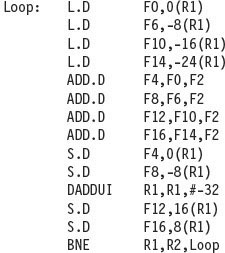
To understand the full power of eliminating WAW and WAR hazards through dynamic renaming of registers, we must look at a loop. Consider the following simple sequence for multiplying the elements of an array by a scalar in F2:

If we predict that branches are taken, using reservation stations will allow multiple executions of this loop to proceed at once. This advantage is gained without changing the code—in effect, the loop is unrolled dynamically by the hardware using the reservation stations obtained by renaming to act as additional registers.

Let’s assume we have issued all the instructions in two successive iterations of the loop, but none of the floating-point load/stores or operations has completed. Figure 3.10 shows reservation stations, register status tables, and load and store buffers at this point. (The integer ALU operation is ignored, and it is assumed the branch was predicted as taken.) Once the system reaches this state, two copies of the loop could be sustained with a CPI close to 1.0, provided the multiplies could complete in four clock cycles. With a latency of six cycles, additional iterations will need to be processed before the steady state can be reached. This requires more reservation stations to hold instructions that are in execution. As we will see later in this chapter, when extended with multiple instruction issue, Tomasulo’s approach can sustain more than one instruction per clock.

Figure 3.10 Two active iterations of the loop with no instruction yet completed. Entries in the multiplier reservation stations indicate that the outstanding loads are the sources. The store reservation stations indicate that the multiply destination is the source of the value to store.

A load and a store can safely be done out of order, provided they access different addresses. If a load and a store access the same address, then either

The load is before the store in program order and interchanging them results in a WAR hazard, or

The store is before the load in program order and interchanging them results in a RAW hazard.

Similarly, interchanging two stores to the same address results in a WAW hazard.

Hence, to determine if a load can be executed at a given time, the processor can check whether any uncompleted store that precedes the load in program order shares the same data memory address as the load. Similarly, a store must wait until there are no unexecuted loads or stores that are earlier in program order and share the same data memory address. We consider a method to eliminate this restriction in Section 3.9.

To detect such hazards, the processor must have computed the data memory address associated with any earlier memory operation. A simple, but not necessarily optimal, way to guarantee that the processor has all such addresses is to perform the effective address calculations in program order. (We really only need to keep the relative order between stores and other memory references; that is, loads can be reordered freely.)

Let’s consider the situation of a load first. If we perform effective address calculation in program order, then when a load has completed effective address calculation, we can check whether there is an address conflict by examining the A field of all active store buffers. If the load address matches the address of any active entries in the store buffer, that load instruction is not sent to the load buffer until the conflicting store completes. (Some implementations bypass the value directly to the load from a pending store, reducing the delay for this RAW hazard.)

Stores operate similarly, except that the processor must check for conflicts in both the load buffers and the store buffers, since conflicting stores cannot be reordered with respect to either a load or a store.

A dynamically scheduled pipeline can yield very high performance, provided branches are predicted accurately—an issue we addressed in the last section. The major drawback of this approach is the complexity of the Tomasulo scheme, which requires a large amount of hardware. In particular, each reservation station must contain an associative buffer, which must run at high speed, as well as complex control logic. The performance can also be limited by the single CDB. Although additional CDBs can be added, each CDB must interact with each reservation station, and the associative tag-matching hardware would have to be duplicated at each station for each CDB.

In Tomasulo’s scheme, two different techniques are combined: the renaming of the architectural registers to a larger set of registers and the buffering of source operands from the register file. Source operand buffering resolves WAR hazards that arise when the operand is available in the registers. As we will see later, it is also possible to eliminate WAR hazards by the renaming of a register together with the buffering of a result until no outstanding references to the earlier version of the register remain. This approach will be used when we discuss hardware speculation.

Tomasulo’s scheme was unused for many years after the 360/91, but was widely adopted in multiple-issue processors starting in the 1990s for several reasons:

The Basic VLIW Approach

VLIWs use multiple, independent functional units. Rather than attempting to issue multiple, independent instructions to the units, a VLIW packages the multiple operations into one very long instruction, or requires that the instructions in the issue packet satisfy the same constraints. Since there is no fundamental difference in the two approaches, we will just assume that multiple operations are placed in one instruction, as in the original VLIW approach.

Since the advantage of a VLIW increases as the maximum issue rate grows, we focus on a wider issue processor. Indeed, for simple two-issue processors, the overhead of a superscalar is probably minimal. Many designers would probably argue that a four-issue processor has manageable overhead, but as we will see later in this chapter, the growth in overhead is a major factor limiting wider issue processors.

Let’s consider a VLIW processor with instructions that contain five operations, including one integer operation (which could also be a branch), two floating-point operations, and two memory references. The instruction would have a set of fields for each functional unit—perhaps 16 to 24 bits per unit, yielding an instruction length of between 80 and 120 bits. By comparison, the Intel Itanium 1 and 2 contain six operations per instruction packet (i.e., they allow concurrent issue of two three-instruction bundles, as Appendix H describes).

To keep the functional units busy, there must be enough parallelism in a code sequence to fill the available operation slots. This parallelism is uncovered by unrolling loops and scheduling the code within the single larger loop body. If the unrolling generates straight-line code, then local scheduling techniques, which operate on a single basic block, can be used. If finding and exploiting the parallelism require scheduling code across branches, a substantially more complex global scheduling algorithm must be used. Global scheduling algorithms are not only more complex in structure, but they also must deal with significantly more complicated trade-offs in optimization, since moving code across branches is expensive.

In Appendix H, we will discuss trace scheduling, one of these global scheduling techniques developed specifically for VLIWs; we will also explore special hardware support that allows some conditional branches to be eliminated, extending the usefulness of local scheduling and enhancing the performance of global scheduling.

For now, we will rely on loop unrolling to generate long, straight-line code sequences, so that we can use local scheduling to build up VLIW instructions and focus on how well these processors operate.

Example

Suppose we have a VLIW that could issue two memory references, two FP operations, and one integer operation or branch in every clock cycle. Show an unrolled version of the loop x[i] = x[i] + s (see page 158 for the MIPS code) for such a processor. Unroll as many times as necessary to eliminate any stalls. Ignore delayed branches.

Answer

Figure 3.16 shows the code. The loop has been unrolled to make seven copies of the body, which eliminates all stalls (i.e., completely empty issue cycles), and runs in 9 cycles. This code yields a running rate of seven results in 9 cycles, or 1.29 cycles per result, nearly twice as fast as the two-issue superscalar of Section 3.2 that used unrolled and scheduled code.

Figure 3.16 VLIW instructions that occupy the inner loop and replace the unrolled sequence. This code takes 9 cycles assuming no branch delay; normally the branch delay would also need to be scheduled. The issue rate is 23 operations in 9 clock cycles, or 2.5 operations per cycle. The efficiency, the percentage of available slots that contained an operation, is about 60%. To achieve this issue rate requires a larger number of registers than MIPS would normally use in this loop. The VLIW code sequence above requires at least eight FP registers, while the same code sequence for the base MIPS processor can use as few as two FP registers or as many as five when unrolled and scheduled.

For the original VLIW model, there were both technical and logistical problems that make the approach less efficient. The technical problems are the increase in code size and the limitations of lockstep operation. Two different elements combine to increase code size substantially for a VLIW. First, generating enough operations in a straight-line code fragment requires ambitiously unrolling loops (as in earlier examples), thereby increasing code size. Second, whenever instructions are not full, the unused functional units translate to wasted bits in the instruction encoding. In Appendix H, we examine software scheduling approaches, such as software pipelining, that can achieve the benefits of unrolling without as much code expansion.

To combat this code size increase, clever encodings are sometimes used. For example, there may be only one large immediate field for use by any functional unit. Another technique is to compress the instructions in main memory and expand them when they are read into the cache or are decoded. In Appendix H, we show other techniques, as well as document the significant code expansion seen on IA-64.

Early VLIWs operated in lockstep; there was no hazard-detection hardware at all. This structure dictated that a stall in any functional unit pipeline must cause the entire processor to stall, since all the functional units must be kept synchronized. Although a compiler may be able to schedule the deterministic functional units to prevent stalls, predicting which data accesses will encounter a cache stall and scheduling them are very difficult. Hence, caches needed to be blocking and to cause all the functional units to stall. As the issue rate and number of memory references becomes large, this synchronization restriction becomes unacceptable. In more recent processors, the functional units operate more independently, and the compiler is used to avoid hazards at issue time, while hardware checks allow for unsynchronized execution once instructions are issued.

Binary code compatibility has also been a major logistical problem for VLIWs. In a strict VLIW approach, the code sequence makes use of both the instruction set definition and the detailed pipeline structure, including both functional units and their latencies. Thus, different numbers of functional units and unit latencies require different versions of the code. This requirement makes migrating between successive implementations, or between implementations with different issue widths, more difficult than it is for a superscalar design. Of course, obtaining improved performance from a new superscalar design may require recompilation. Nonetheless, the ability to run old binary files is a practical advantage for the superscalar approach.

The EPIC approach, of which the IA-64 architecture is the primary example, provides solutions to many of the problems encountered in early VLIW designs, including extensions for more aggressive software speculation and methods to overcome the limitation of hardware dependence while preserving binary compatibility.

The major challenge for all multiple-issue processors is to try to exploit large amounts of ILP. When the parallelism comes from unrolling simple loops in FP programs, the original loop probably could have been run efficiently on a vector processor (described in the next chapter). It is not clear that a multiple-issue processor is preferred over a vector processor for such applications; the costs are similar, and the vector processor is typically the same speed or faster. The potential advantages of a multiple-issue processor versus a vector processor are their ability to extract some parallelism from less structured code and their ability to easily cache all forms of data. For these reasons multiple-issue approaches have become the primary method for taking advantage of instruction-level parallelism, and vectors have become primarily an extension to these processors.