
3.9 Advanced Techniques for Instruction Delivery and Speculation
In a high-performance pipeline, especially one with multiple issues, predicting branches well is not enough; we actually have to be able to deliver a high-bandwidth instruction stream. In recent multiple-issue processors, this has meant delivering 4 to 8 instructions every clock cycle. We look at methods for increasing instruction delivery bandwidth first. We then turn to a set of key issues in implementing advanced speculation techniques, including the use of register renaming versus reorder buffers, the aggressiveness of speculation, and a technique called value prediction, which attempts to predict the result of a computation and which could further enhance ILP.
Increasing Instruction Fetch Bandwidth
A multiple-issue processor will require that the average number of instructions fetched every clock cycle be at least as large as the average throughput. Of course, fetching these instructions requires wide enough paths to the instruction cache, but the most difficult aspect is handling branches. In this section, we look at two methods for dealing with branches and then discuss how modern processors integrate the instruction prediction and prefetch functions.
Branch-Target Buffers
To reduce the branch penalty for our simple five-stage pipeline, as well as for deeper pipelines, we must know whether the as-yet-undecoded instruction is a branch and, if so, what the next program counter (PC) should be. If the instruction is a branch and we know what the next PC should be, we can have a branch penalty of zero. A branch-prediction cache that stores the predicted address for the next instruction after a branch is called a branch-target buffer or branch-target cache. Figure 3.21 shows a branch-target buffer.

Figure 3.21 A branch-target buffer. The PC of the instruction being fetched is matched against a set of instruction addresses stored in the first column; these represent the addresses of known branches. If the PC matches one of these entries, then the instruction being fetched is a taken branch, and the second field, predicted PC, contains the prediction for the next PC after the branch. Fetching begins immediately at that address. The third field, which is optional, may be used for extra prediction state bits.
Because a branch-target buffer predicts the next instruction address and will send it out before decoding the instruction, we must know whether the fetched instruction is predicted as a taken branch. If the PC of the fetched instruction matches an address in the prediction buffer, then the corresponding predicted PC is used as the next PC. The hardware for this branch-target buffer is essentially identical to the hardware for a cache.
If a matching entry is found in the branch-target buffer, fetching begins immediately at the predicted PC. Note that unlike a branch-prediction buffer, the predictive entry must be matched to this instruction because the predicted PC will be sent out before it is known whether this instruction is even a branch. If the processor did not check whether the entry matched this PC, then the wrong PC would be sent out for instructions that were not branches, resulting in worse performance. We only need to store the predicted-taken branches in the branch-target buffer, since an untaken branch should simply fetch the next sequential instruction, as if it were not a branch.
Figure 3.22 shows the steps when using a branch-target buffer for a simple five-stage pipeline. From this figure we can see that there will be no branch delay if a branch-prediction entry is found in the buffer and the prediction is correct. Otherwise, there will be a penalty of at least two clock cycles. Dealing with the mispredictions and misses is a significant challenge, since we typically will have to halt instruction fetch while we rewrite the buffer entry. Thus, we would like to make this process fast to minimize the penalty.

To evaluate how well a branch-target buffer works, we first must determine the penalties in all possible cases. Figure 3.23 contains this information for a simple five-stage pipeline.

Figure 3.23 Penalties for all possible combinations of whether the branch is in the buffer and what it actually does, assuming we store only taken branches in the buffer. There is no branch penalty if everything is correctly predicted and the branch is found in the target buffer. If the branch is not correctly predicted, the penalty is equal to one clock cycle to update the buffer with the correct information (during which an instruction cannot be fetched) and one clock cycle, if needed, to restart fetching the next correct instruction for the branch. If the branch is not found and taken, a two-cycle penalty is encountered, during which time the buffer is updated.
Example
Determine the total branch penalty for a branch-target buffer assuming the penalty cycles for individual mispredictions from Figure 3.23. Make the following assumptions about the prediction accuracy and hit rate:
Answer
We compute the penalty by looking at the probability of two events: the branch is predicted taken but ends up being not taken, and the branch is taken but is not found in the buffer. Both carry a penalty of two cycles.

This penalty compares with a branch penalty for delayed branches, which we evaluate in Appendix C, of about 0.5 clock cycles per branch. Remember, though, that the improvement from dynamic branch prediction will grow as the pipeline length and, hence, the branch delay grows; in addition, better predictors will yield a larger performance advantage. Modern high-performance processors have branch misprediction delays on the order of 15 clock cycles; clearly, accurate prediction is critical!
One variation on the branch-target buffer is to store one or more target instructions instead of, or in addition to, the predicted target address. This variation has two potential advantages. First, it allows the branch-target buffer access to take longer than the time between successive instruction fetches, possibly allowing a larger branch-target buffer. Second, buffering the actual target instructions allows us to perform an optimization called branch folding. Branch folding can be used to obtain 0-cycle unconditional branches and sometimes 0-cycle conditional branches.
Consider a branch-target buffer that buffers instructions from the predicted path and is being accessed with the address of an unconditional branch. The only function of the unconditional branch is to change the PC. Thus, when the branch-target buffer signals a hit and indicates that the branch is unconditional, the pipeline can simply substitute the instruction from the branch-target buffer in place of the instruction that is returned from the cache (which is the unconditional branch). If the processor is issuing multiple instructions per cycle, then the buffer will need to supply multiple instructions to obtain the maximum benefit. In some cases, it may be possible to eliminate the cost of a conditional branch.
Return Address Predictors
As we try to increase the opportunity and accuracy of speculation we face the challenge of predicting indirect jumps, that is, jumps whose destination address varies at runtime. Although high-level language programs will generate such jumps for indirect procedure calls, select or case statements, and FORTRAN-computed gotos, the vast majority of the indirect jumps come from procedure returns. For example, for the SPEC95 benchmarks, procedure returns account for more than 15% of the branches and the vast majority of the indirect jumps on average. For object-oriented languages such as C++ and Java, procedure returns are even more frequent. Thus, focusing on procedure returns seems appropriate.
Though procedure returns can be predicted with a branch-target buffer, the accuracy of such a prediction technique can be low if the procedure is called from multiple sites and the calls from one site are not clustered in time. For example, in SPEC CPU95, an aggressive branch predictor achieves an accuracy of less than 60% for such return branches. To overcome this problem, some designs use a small buffer of return addresses operating as a stack. This structure caches the most recent return addresses: pushing a return address on the stack at a call and popping one off at a return. If the cache is sufficiently large (i.e., as large as the maximum call depth), it will predict the returns perfectly. Figure 3.24 shows the performance of such a return buffer with 0 to 16 elements for a number of the SPEC CPU95 benchmarks. We will use a similar return predictor when we examine the studies of ILP in Section 3.10. Both the Intel Core processors and the AMD Phenom processors have return address predictors.

Figure 3.24 Prediction accuracy for a return address buffer operated as a stack on a number of SPEC CPU95 benchmarks. The accuracy is the fraction of return addresses predicted correctly. A buffer of 0 entries implies that the standard branch prediction is used. Since call depths are typically not large, with some exceptions, a modest buffer works well. These data come from Skadron et al. [1999] and use a fix-up mechanism to prevent corruption of the cached return addresses.
Integrated Instruction Fetch Units
To meet the demands of multiple-issue processors, many recent designers have chosen to implement an integrated instruction fetch unit as a separate autonomous unit that feeds instructions to the rest of the pipeline. Essentially, this amounts to recognizing that characterizing instruction fetch as a simple single pipe stage given the complexities of multiple issue is no longer valid.
Instead, recent designs have used an integrated instruction fetch unit that integrates several functions:
Virtually all high-end processors now use a separate instruction fetch unit connected to the rest of the pipeline by a buffer containing pending instructions.
Speculation: Implementation Issues and Extensions
In this section we explore four issues that involve the design trade-offs in speculation, starting with the use of register renaming, the approach that is often used instead of a reorder buffer. We then discuss one important possible extension to speculation on control flow: an idea called value prediction.
Speculation Support: Register Renaming versus Reorder Buffers
One alternative to the use of a reorder buffer (ROB) is the explicit use of a larger physical set of registers combined with register renaming. This approach builds on the concept of renaming used in Tomasulo’s algorithm and extends it. In Tomasulo’s algorithm, the values of the architecturally visible registers (R0, …, R31 and F0, …, F31) are contained, at any point in execution, in some combination of the register set and the reservation stations. With the addition of speculation, register values may also temporarily reside in the ROB. In either case, if the processor does not issue new instructions for a period of time, all existing instructions will commit, and the register values will appear in the register file, which directly corresponds to the architecturally visible registers.
In the register-renaming approach, an extended set of physical registers is used to hold both the architecturally visible registers as well as temporary values. Thus, the extended registers replace most of the function of the ROB and the reservation stations; only a queue to ensure that instructions complete in order is needed. During instruction issue, a renaming process maps the names of architectural registers to physical register numbers in the extended register set, allocating a new unused register for the destination. WAW and WAR hazards are avoided by renaming of the destination register, and speculation recovery is handled because a physical register holding an instruction destination does not become the architectural register until the instruction commits. The renaming map is a simple data structure that supplies the physical register number of the register that currently corresponds to the specified architectural register, a function performed by the register status table in Tomasulo’s algorithm. When an instruction commits, the renaming table is permanently updated to indicate that a physical register corresponds to the actual architectural register, thus effectively finalizing the update to the processor state. Although an ROB is not necessary with register renaming, the hardware must still track instructions in a queue-like structure and update the renaming table in strict order.
An advantage of the renaming approach versus the ROB approach is that instruction commit is slightly simplified, since it requires only two simple actions: (1) record that the mapping between an architectural register number and physical register number is no longer speculative, and (2) free up any physical registers being used to hold the “older” value of the architectural register. In a design with reservation stations, a station is freed up when the instruction using it completes execution, and a ROB entry is freed up when the corresponding instruction commits.
With register renaming, deallocating registers is more complex, since before we free up a physical register, we must know that it no longer corresponds to an architectural register and that no further uses of the physical register are outstanding. A physical register corresponds to an architectural register until the architectural register is rewritten, causing the renaming table to point elsewhere. That is, if no renaming entry points to a particular physical register, then it no longer corresponds to an architectural register. There may, however, still be uses of the physical register outstanding. The processor can determine whether this is the case by examining the source register specifiers of all instructions in the functional unit queues. If a given physical register does not appear as a source and it is not designated as an architectural register, it may be reclaimed and reallocated.
Alternatively, the processor can simply wait until another instruction that writes the same architectural register commits. At that point, there can be no further uses of the older value outstanding. Although this method may tie up a physical register slightly longer than necessary, it is easy to implement and is used in most recent superscalars.
One question you may be asking is how do we ever know which registers are the architectural registers if they are constantly changing? Most of the time when the program is executing, it does not matter. There are clearly cases, however, where another process, such as the operating system, must be able to know exactly where the contents of a certain architectural register reside. To understand how this capability is provided, assume the processor does not issue instructions for some period of time. Eventually all instructions in the pipeline will commit, and the mapping between the architecturally visible registers and physical registers will become stable. At that point, a subset of the physical registers contains the architecturally visible registers, and the value of any physical register not associated with an architectural register is unneeded. It is then easy to move the architectural registers to a fixed subset of physical registers so that the values can be communicated to another process.
Both register renaming and reorder buffers continue to be used in high-end processors, which now feature the ability to have as many as 40 or 50 instructions (including loads and stores waiting on the cache) in flight. Whether renaming or a reorder buffer is used, the key complexity bottleneck for a dynamically schedule superscalar remains issuing bundles of instructions with dependences within the bundle. In particular, dependent instructions in an issue bundle must be issued with the assigned virtual registers of the instructions on which they depend. A strategy for instruction issue with register renaming similar to that used for multiple issue with reorder buffers (see page 198) can be deployed, as follows:
Note that just as in the reorder buffer case, the issue logic must both determine dependences within the bundle and update the renaming tables in a single clock, and, as before, the complexity of doing this for a larger number of instructions per clock becomes a chief limitation in the issue width.
How Much to Speculate
One of the significant advantages of speculation is its ability to uncover events that would otherwise stall the pipeline early, such as cache misses. This potential advantage, however, comes with a significant potential disadvantage. Speculation is not free. It takes time and energy, and the recovery of incorrect speculation further reduces performance. In addition, to support the higher instruction execution rate needed to benefit from speculation, the processor must have additional resources, which take silicon area and power. Finally, if speculation causes an exceptional event to occur, such as a cache or translation lookaside buffer (TLB) miss, the potential for significant performance loss increases, if that event would not have occurred without speculation.
To maintain most of the advantage, while minimizing the disadvantages, most pipelines with speculation will allow only low-cost exceptional events (such as a first-level cache miss) to be handled in speculative mode. If an expensive exceptional event occurs, such as a second-level cache miss or a TLB miss, the processor will wait until the instruction causing the event is no longer speculative before handling the event. Although this may slightly degrade the performance of some programs, it avoids significant performance losses in others, especially those that suffer from a high frequency of such events coupled with less-than-excellent branch prediction.
In the 1990s, the potential downsides of speculation were less obvious. As processors have evolved, the real costs of speculation have become more apparent, and the limitations of wider issue and speculation have been obvious. We return to this issue shortly.
Speculating through Multiple Branches
In the examples we have considered in this chapter, it has been possible to resolve a branch before having to speculate on another. Three different situations can benefit from speculating on multiple branches simultaneously: (1) a very high branch frequency, (2) significant clustering of branches, and (3) long delays in functional units. In the first two cases, achieving high performance may mean that multiple branches are speculated, and it may even mean handling more than one branch per clock. Database programs, and other less structured integer computations, often exhibit these properties, making speculation on multiple branches important. Likewise, long delays in functional units can raise the importance of speculating on multiple branches as a way to avoid stalls from the longer pipeline delays.
Speculating on multiple branches slightly complicates the process of speculation recovery but is straightforward otherwise. As of 2011, no processor has yet combined full speculation with resolving multiple branches per cycle, and it is unlikely that the costs of doing so would be justified in terms of performance versus complexity and power.
Speculation and the Challenge of Energy Efficiency
What is the impact of speculation on energy efficiency? At first glance, one might argue that using speculation always decreases energy efficiency, since whenever speculation is wrong it consumes excess energy in two ways:
Certainly, speculation will raise the power consumption and, if we could control speculation, it would be possible to measure the cost (or at least the dynamic power cost). But, if speculation lowers the execution time by more than it increases the average power consumption, then the total energy consumed may be less.
Thus, to understand the impact of speculation on energy efficiency, we need to look at how often speculation is leading to unnecessary work. If a significant number of unneeded instructions is executed, it is unlikely that speculation will improve running time by a comparable amount! Figure 3.25 shows the fraction of instructions that are executed from misspeculation. As we can see, this fraction is small in scientific code and significant (about 30% on average) in integer code. Thus, it is unlikely that speculation is energy efficient for integer applications. Designers could avoid speculation, try to reduce the misspeculation, or think about new approaches, such as only speculating on branches that are known to be highly predictable.

Value Prediction
One technique for increasing the amount of ILP available in a program is value prediction. Value prediction attempts to predict the value that will be produced by an instruction. Obviously, since most instructions produce a different value every time they are executed (or at least a different value from a set of values), value prediction can have only limited success. There are, however, certain instructions for which it is easier to predict the resulting value—for example, loads that load from a constant pool or that load a value that changes infrequently. In addition, when an instruction produces a value chosen from a small set of potential values, it may be possible to predict the resulting value by correlating it with other program behavior.
Value prediction is useful if it significantly increases the amount of available ILP. This possibility is most likely when a value is used as the source of a chain of dependent computations, such as a load. Because value prediction is used to enhance speculations and incorrect speculation has detrimental performance impact, the accuracy of the prediction is critical.
Although many researchers have focused on value prediction in the past ten years, the results have never been sufficiently attractive to justify their incorporation in real processors. Instead, a simpler and older idea, related to value prediction, has been used: address aliasing prediction. Address aliasing prediction is a simple technique that predicts whether two stores or a load and a store refer to the same memory address. If two such references do not refer to the same address, then they may be safely interchanged. Otherwise, we must wait until the memory addresses accessed by the instructions are known. Because we need not actually predict the address values, only whether such values conflict, the prediction is both more stable and simpler. This limited form of address value speculation has been used in several processors already and may become universal in the future.
3.10 Studies of the Limitations of ILP
Exploiting ILP to increase performance began with the first pipelined processors in the 1960s. In the 1980s and 1990s, these techniques were key to achieving rapid performance improvements. The question of how much ILP exists was critical to our long-term ability to enhance performance at a rate that exceeds the increase in speed of the base integrated circuit technology. On a shorter scale, the critical question of what is needed to exploit more ILP is crucial to both computer designers and compiler writers. The data in this section also provide us with a way to examine the value of ideas that we have introduced in this chapter, including memory disambiguation, register renaming, and speculation.
In this section we review a portion of one of the studies done of these questions (based on Wall’s 1993 study). All of these studies of available parallelism operate by making a set of assumptions and seeing how much parallelism is available under those assumptions. The data we examine here are from a study that makes the fewest assumptions; in fact, the ultimate hardware model is probably unrealizable. Nonetheless, all such studies assume a certain level of compiler technology, and some of these assumptions could affect the results, despite the use of incredibly ambitious hardware.
As we will see, for hardware models that have reasonable cost, it is unlikely that the costs of very aggressive speculation can be justified: the inefficiencies in power and use of silicon are simply too high. While many in the research community and the major processor manufacturers were betting in favor of much greater exploitable ILP and were initially reluctant to accept this possibility, by 2005 they were forced to change their minds.
The Hardware Model
To see what the limits of ILP might be, we first need to define an ideal processor. An ideal processor is one where all constraints on ILP are removed. The only limits on ILP in such a processor are those imposed by the actual data flows through either registers or memory.
The assumptions made for an ideal or perfect processor are as follows:
Assumptions 2 and 3 eliminate all control dependences. Likewise, assumptions 1 and 4 eliminate all but the true data dependences. Together, these four assumptions mean that any instruction in the program’s execution can be scheduled on the cycle immediately following the execution of the predecessor on which it depends. It is even possible, under these assumptions, for the last dynamically executed instruction in the program to be scheduled on the very first cycle! Thus, this set of assumptions subsumes both control and address speculation and implements them as if they were perfect.
Initially, we examine a processor that can issue an unlimited number of instructions at once, looking arbitrarily far ahead in the computation. For all the processor models we examine, there are no restrictions on what types of instructions can execute in a cycle. For the unlimited-issue case, this means there may be an unlimited number of loads or stores issuing in one clock cycle. In addition, all functional unit latencies are assumed to be one cycle, so that any sequence of dependent instructions can issue on successive cycles. Latencies longer than one cycle would decrease the number of issues per cycle, although not the number of instructions under execution at any point. (The instructions in execution at any point are often referred to as in flight.)
Of course, this ideal processor is probably unrealizable. For example, the IBM Power7 (see Wendell et. al. [2010]) is the most advanced superscalar processor announced to date. The Power7 issues up to six instructions per clock and initiates execution on up to 8 of 12 execution units (only two of which are load/store units), supports a large set of renaming registers (allowing hundreds of instructions to be in flight), uses a large aggressive branch predictor, and employs dynamic memory disambiguation. The Power7 continued the move toward using more thread-level parallelism by increasing the width of simultaneous multithreading (SMT) support (to four threads per core) and the number of cores per chip to eight. After looking at the parallelism available for the perfect processor, we will examine what might be achievable in any processor likely to be designed in the near future.
To measure the available parallelism, a set of programs was compiled and optimized with the standard MIPS optimizing compilers. The programs were instrumented and executed to produce a trace of the instruction and data references. Every instruction in the trace is then scheduled as early as possible, limited only by the data dependences. Since a trace is used, perfect branch prediction and perfect alias analysis are easy to do. With these mechanisms, instructions may be scheduled much earlier than they would otherwise, moving across large numbers of instructions on which they are not data dependent, including branches, since branches are perfectly predicted.
Figure 3.26 shows the average amount of parallelism available for six of the SPEC92 benchmarks. Throughout this section the parallelism is measured by the average instruction issue rate. Remember that all instructions have a one-cycle latency; a longer latency would reduce the average number of instructions per clock. Three of these benchmarks (fpppp, doduc, and tomcatv) are floating-point intensive, and the other three are integer programs. Two of the floating-point benchmarks (fpppp and tomcatv) have extensive parallelism, which could be exploited by a vector computer or by a multiprocessor (the structure in fpppp is quite messy, however, since some hand transformations have been done on the code). The doduc program has extensive parallelism, but the parallelism does not occur in simple parallel loops as it does in fpppp and tomcatv. The program li is a LISP interpreter that has many short dependences.

Limitations on ILP for Realizable Processors
In this section we look at the performance of processors with ambitious levels of hardware support equal to or better than what is available in 2011 or, given the events and lessons of the last decade, likely to be available in the near future. In particular, we assume the following fixed attributes:
Figure 3.27 shows the result for this configuration as we vary the window size. This configuration is more complex and expensive than any existing implementations, especially in terms of the number of instruction issues, which is more than 10 times larger than the largest number of issues available on any processor in 2011. Nonetheless, it gives a useful bound on what future implementations might yield. The data in these figures are likely to be very optimistic for another reason. There are no issue restrictions among the 64 instructions: They may all be memory references. No one would even contemplate this capability in a processor in the near future. Unfortunately, it is quite difficult to bound the performance of a processor with reasonable issue restrictions; not only is the space of possibilities quite large, but the existence of issue restrictions requires that the parallelism be evaluated with an accurate instruction scheduler, making the cost of studying processors with large numbers of issues very expensive.

Figure 3.27 The amount of parallelism available versus the window size for a variety of integer and floating-point programs with up to 64 arbitrary instruction issues per clock. Although there are fewer renaming registers than the window size, the fact that all operations have one-cycle latency and the number of renaming registers equals the issue width allows the processor to exploit parallelism within the entire window. In a real implementation, the window size and the number of renaming registers must be balanced to prevent one of these factors from overly constraining the issue rate.
In addition, remember that in interpreting these results cache misses and non-unit latencies have not been taken into account, and both these effects will have significant impact!
The most startling observation from Figure 3.27 is that, with the realistic processor constraints listed above, the effect of the window size for the integer programs is not as severe as for FP programs. This result points to the key difference between these two types of programs. The availability of loop-level parallelism in two of the FP programs means that the amount of ILP that can be exploited is higher, but for integer programs other factors—such as branch prediction, register renaming, and less parallelism, to start with—are all important limitations. This observation is critical because of the increased emphasis on integer performance since the explosion of the World Wide Web and cloud computing starting in the mid-1990s. Indeed, most of the market growth in the last decade—transaction processing, Web servers, and the like—depended on integer performance, rather than floating point. As we will see in the next section, for a realistic processor in 2011, the actual performance levels are much lower than those shown in Figure 3.27.
Given the difficulty of increasing the instruction rates with realistic hardware designs, designers face a challenge in deciding how best to use the limited resources available on an integrated circuit. One of the most interesting trade-offs is between simpler processors with larger caches and higher clock rates versus more emphasis on instruction-level parallelism with a slower clock and smaller caches. The following example illustrates the challenges, and in the next chapter we will see an alternative approach to exploiting fine-grained parallelism in the form of GPUs.
Example
Consider the following three hypothetical, but not atypical, processors, which we run with the SPEC gcc benchmark:
Assume that the main memory time (which sets the miss penalty) is 50 ns. Determine the relative performance of these three processors.
Answer
First, we use the miss penalty and miss rate information to compute the contribution to CPI from cache misses for each configuration. We do this with the following formula:
We need to compute the miss penalties for each system:
The clock cycle times for the processors are 250 ps, 200 ps, and 400 ps, respectively. Hence, the miss penalties are

Applying this for each cache:

We know the pipeline CPI contribution for everything but processor 3; its pipeline CPI is given by:
Now we can find the CPI for each processor by adding the pipeline and cache CPI contributions:

Since this is the same architecture, we can compare instruction execution rates in millions of instructions per second (MIPS) to determine relative performance:

In this example, the simple two-issue static superscalar looks best. In practice, performance depends on both the CPI and clock rate assumptions.
Beyond the Limits of This Study
Like any limit study, the study we have examined in this section has its own limitations. We divide these into two classes: limitations that arise even for the perfect speculative processor, and limitations that arise for one or more realistic models. Of course, all the limitations in the first class apply to the second. The most important limitations that apply even to the perfect model are
For a less-than-perfect processor, several ideas have been proposed that could expose more ILP. One example is to speculate along multiple paths. This idea was discussed by Lam and Wilson [1992] and explored in the study covered in this section. By speculating on multiple paths, the cost of incorrect recovery is reduced and more parallelism can be uncovered. It only makes sense to evaluate this scheme for a limited number of branches because the hardware resources required grow exponentially. Wall [1993] provided data for speculating in both directions on up to eight branches. Given the costs of pursuing both paths, knowing that one will be thrown away (and the growing amount of useless computation as such a process is followed through multiple branches), every commercial design has instead devoted additional hardware to better speculation on the correct path.
It is critical to understand that none of the limits in this section is fundamental in the sense that overcoming them requires a change in the laws of physics! Instead, they are practical limitations that imply the existence of some formidable barriers to exploiting additional ILP. These limitations—whether they be window size, alias detection, or branch prediction—represent challenges for designers and researchers to overcome.
Attempts to break through these limits in the first five years of this century met with frustration. Some techniques produced small improvements, but often at significant increases in complexity, increases in the clock cycle, and disproportionate increases in power. In summary, designers discovered that trying to extract more ILP was simply too inefficient. We will return to this discussion in our concluding remarks.
3.11 Cross-Cutting Issues: ILP Approaches and the Memory System
Hardware versus Software Speculation
The hardware-intensive approaches to speculation in this chapter and the software approaches of Appendix H provide alternative approaches to exploiting ILP. Some of the trade-offs, and the limitations, for these approaches are listed below:
The major disadvantage of supporting speculation in hardware is the complexity and additional hardware resources required. This hardware cost must be evaluated against both the complexity of a compiler for a software-based approach and the amount and usefulness of the simplifications in a processor that relies on such a compiler.
Some designers have tried to combine the dynamic and compiler-based approaches to achieve the best of each. Such a combination can generate interesting and obscure interactions. For example, if conditional moves are combined with register renaming, a subtle side effect appears. A conditional move that is annulled must still copy a value to the destination register, since it was renamed earlier in the instruction pipeline. These subtle interactions complicate the design and verification process and can also reduce performance.
The Intel Itanium processor was the most ambitious computer ever designed based on the software support for ILP and speculation. It did not deliver on the hopes of the designers, especially for general-purpose, nonscientific code. As designers’ ambitions for exploiting ILP were reduced in light of the difficulties discussed in Section 3.10, most architectures settled on hardware-based mechanisms with issue rates of three to four instructions per clock.
Speculative Execution and the Memory System
Inherent in processors that support speculative execution or conditional instructions is the possibility of generating invalid addresses that would not occur without speculative execution. Not only would this be incorrect behavior if protection exceptions were taken, but the benefits of speculative execution would be swamped by false exception overhead. Hence, the memory system must identify speculatively executed instructions and conditionally executed instructions and suppress the corresponding exception.
By similar reasoning, we cannot allow such instructions to cause the cache to stall on a miss because again unnecessary stalls could overwhelm the benefits of speculation. Hence, these processors must be matched with nonblocking caches.
In reality, the penalty of an L2 miss is so large that compilers normally only speculate on L1 misses. Figure 2.5 on page 84 shows that for some well-behaved scientific programs the compiler can sustain multiple outstanding L2 misses to cut the L2 miss penalty effectively. Once again, for this to work the memory system behind the cache must match the goals of the compiler in number of simultaneous memory accesses.
3.12 Multithreading: Exploiting Thread-Level Parallelism to Improve Uniprocessor Throughput
The topic we cover in this section, multithreading, is truly a cross-cutting topic, since it has relevance to pipelining and superscalars, to graphics processing units (Chapter 4), and to multiprocessors (Chapter 5). We introduce the topic here and explore the use of multithreading to increase uniprocessor throughput by using multiple threads to hide pipeline and memory latencies. In the next chapter, we will see how multithreading provides the same advantages in GPUs, and finally, Chapter 5 will explore the combination of multithreading and multiprocessing. These topics are closely interwoven, since multithreading is a primary technique for exposing more parallelism to the hardware. In a strict sense, multithreading uses thread-level parallelism, and thus is properly the subject of Chapter 5, but its role in both improving pipeline utilization and in GPUs motivates us to introduce the concept here.
Although increasing performance by using ILP has the great advantage that it is reasonably transparent to the programmer, as we have seen ILP can be quite limited or difficult to exploit in some applications. In particular, with reasonable instruction issue rates, cache misses that go to memory or off-chip caches are unlikely to be hidden by available ILP. Of course, when the processor is stalled waiting on a cache miss, the utilization of the functional units drops dramatically.
Since attempts to cover long memory stalls with more ILP have limited effectiveness, it is natural to ask whether other forms of parallelism in an application could be used to hide memory delays. For example, an online transaction-processing system has natural parallelism among the multiple queries and updates that are presented by requests. Of course, many scientific applications contain natural parallelism since they often model the three-dimensional, parallel structure of nature, and that structure can be exploited by using separate threads. Even desktop applications that use modern Windows-based operating systems often have multiple active applications running, providing a source of parallelism.
Multithreading allows multiple threads to share the functional units of a single processor in an overlapping fashion. In contrast, a more general method to exploit thread-level parallelism (TLP) is with a multiprocessor that has multiple independent threads operating at once and in parallel. Multithreading, however, does not duplicate the entire processor as a multiprocessor does. Instead, multithreading shares most of the processor core among a set of threads, duplicating only private state, such as the registers and program counter. As we will see in Chapter 5, many recent processors incorporate both multiple processor cores on a single chip and provide multithreading within each core.
Duplicating the per-thread state of a processor core means creating a separate register file, a separate PC, and a separate page table for each thread. The memory itself can be shared through the virtual memory mechanisms, which already support multiprogramming. In addition, the hardware must support the ability to change to a different thread relatively quickly; in particular, a thread switch should be much more efficient than a process switch, which typically requires hundreds to thousands of processor cycles. Of course, for multithreading hardware to achieve performance improvements, a program must contain multiple threads (we sometimes say that the application is multithreaded) that could execute in concurrent fashion. These threads are identified either by a compiler (typically from a language with parallelism constructs) or by the programmer.
There are three main hardware approaches to multithreading. Fine-grained multithreading switches between threads on each clock, causing the execution of instructions from multiple threads to be interleaved. This interleaving is often done in a round-robin fashion, skipping any threads that are stalled at that time. One key advantage of fine-grained multithreading is that it can hide the throughput losses that arise from both short and long stalls, since instructions from other threads can be executed when one thread stalls, even if the stall is only for a few cycles. The primary disadvantage of fine-grained multithreading is that it slows down the execution of an individual thread, since a thread that is ready to execute without stalls will be delayed by instructions from other threads. It trades an uncrease in multithreaded throughput for a loss in the performance (as measured by latency) of a single thread. The Sun Niagara processor, which we examine shortly, uses simple fine-grained multithreading, as do the Nvidia GPUs, which we look at in the next chapter.
Coarse-grained multithreading was invented as an alternative to fine-grained multithreading. Coarse-grained multithreading switches threads only on costly stalls, such as level two or three cache misses. This change relieves the need to have thread-switching be essentially free and is much less likely to slow down the execution of any one thread, since instructions from other threads will only be issued when a thread encounters a costly stall.
Coarse-grained multithreading suffers, however, from a major drawback: It is limited in its ability to overcome throughput losses, especially from shorter stalls. This limitation arises from the pipeline start-up costs of coarse-grained multithreading. Because a CPU with coarse-grained multithreading issues instructions from a single thread, when a stall occurs the pipeline will see a bubble before the new thread begins executing. Because of this start-up overhead, coarse-grained multithreading is much more useful for reducing the penalty of very high-cost stalls, where pipeline refill is negligible compared to the stall time. Several research projects have explored coarse grained multithreading, but no major current processors use this technique.
The most common implementation of multithreading is called Simultaneous multithreading (SMT). Simultaneous multithreading is a variation on fine-grained multithreading that arises naturally when fine-grained multithreading is implemented on top of a multiple-issue, dynamically scheduled processor. As with other forms of multithreading, SMT uses thread-level parallelism to hide long-latency events in a processor, thereby increasing the usage of the functional units. The key insight in SMT is that register renaming and dynamic scheduling allow multiple instructions from independent threads to be executed without regard to the dependences among them; the resolution of the dependences can be handled by the dynamic scheduling capability.
Figure 3.28 conceptually illustrates the differences in a processor’s ability to exploit the resources of a superscalar for the following processor configurations:

Figure 3.28 How four different approaches use the functional unit execution slots of a superscalar processor. The horizontal dimension represents the instruction execution capability in each clock cycle. The vertical dimension represents a sequence of clock cycles. An empty (white) box indicates that the corresponding execution slot is unused in that clock cycle. The shades of gray and black correspond to four different threads in the multithreading processors. Black is also used to indicate the occupied issue slots in the case of the superscalar without multithreading support. The Sun T1 and T2 (aka Niagara) processors are fine-grained multithreaded processors, while the Intel Core i7 and IBM Power7 processors use SMT. The T2 has eight threads, the Power7 has four, and the Intel i7 has two. In all existing SMTs, instructions issue from only one thread at a time. The difference in SMT is that the subsequent decision to execute an instruction is decoupled and could execute the operations coming from several different instructions in the same clock cycle.
In the superscalar without multithreading support, the use of issue slots is limited by a lack of ILP, including ILP to hide memory latency. Because of the length of L2 and L3 cache misses, much of the processor can be left idle.
In the coarse-grained multithreaded superscalar, the long stalls are partially hidden by switching to another thread that uses the resources of the processor. This switching reduces the number of completely idle clock cycles. In a coarse-grained multithreaded processor, however, thread switching only occurs when there is a stall. Because the new thread has a start-up period, there are likely to be some fully idle cycles remaining.
In the fine-grained case, the interleaving of threads can eliminate fully empty slots. In addition, because the issuing thread is changed on every clock cycle, longer latency operations can be hidden. Because instruction issue and execution are connected, a thread can only issue as many instructions as are ready. With a narrow issue width this is not a problem (a cycle is either occupied or not), which is why fine-grained multithreading works perfectly for a single issue processor, and SMT would make no sense. Indeed, in the Sun T2, there are two issues per clock, but they are from different threads. This eliminates the need to implement the complex dynamic scheduling approach and relies instead on hiding latency with more threads.
If one implements fine-grained threading on top of a multiple-issue dynamically schedule processor, the result is SMT. In all existing SMT implementations, all issues come from one thread, although instructions from different threads can initiate execution in the same cycle, using the dynamic scheduling hardware to determine what instructions are ready. Although Figure 3.28 greatly simplifies the real operation of these processors, it does illustrate the potential performance advantages of multithreading in general and SMT in wider issue, dynamically scheduled processors.
Simultaneous multithreading uses the insight that a dynamically scheduled processor already has many of the hardware mechanisms needed to support the mechanism, including a large virtual register set. Multithreading can be built on top of an out-of-order processor by adding a per-thread renaming table, keeping separate PCs, and providing the capability for instructions from multiple threads to commit.
Effectiveness of Fine-Grained Multithreading on the Sun T1
In this section, we use the Sun T1 processor to examine the ability of multithreading to hide latency. The T1 is a fine-grained multithreaded multicore microprocessor introduced by Sun in 2005. What makes T1 especially interesting is that it is almost totally focused on exploiting thread-level parallelism (TLP) rather than instruction-level parallelism (ILP). The T1 abandoned the intense focus on ILP (just shortly after the most aggressive ILP processors ever were introduced), returned to a simple pipeline strategy, and focused on exploiting TLP, using both multiple cores and multithreading to produce throughput.
Each T1 processor contains eight processor cores, each supporting four threads. Each processor core consists of a simple six-stage, single-issue pipeline (a standard five-stage RISC pipeline like that of Appendix C, with one stage added for thread switching). T1 uses fine-grained multithreading (but not SMT), switching to a new thread on each clock cycle, and threads that are idle because they are waiting due to a pipeline delay or cache miss are bypassed in the scheduling. The processor is idle only when all four threads are idle or stalled. Both loads and branches incur a three-cycle delay that can only be hidden by other threads. A single set of floating-point functional units is shared by all eight cores, as floating-point performance was not a focus for T1. Figure 3.29 summarizes the T1 processor.

T1 Multithreading Unicore Performance
The T1 makes TLP its focus, both through the multithreading on an individual core and through the use of many simple cores on a single die. In this section, we will look at the effectiveness of the T1 in increasing the performance of a single core through fine-grained multithreading. In Chapter 5, we will return to examine the effectiveness of combining multithreading with multiple cores.
To examine the performance of the T1, we use three server-oriented benchmarks: TPC-C, SPECJBB (the SPEC Java Business Benchmark), and SPECWeb99. Since multiple threads increase the memory demands from a single processor, they could overload the memory system, leading to reductions in the potential gain from multithreading. Figure 3.30 shows the relative increase in the miss rate and the observed miss latency when executing with one thread per core versus executing four threads per core for TPC-C. Both the miss rates and the miss latencies increase, due to increased contention in the memory system. The relatively small increase in miss latency indicates that the memory system still has unused capacity.
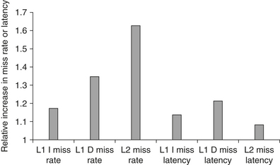
Figure 3.30 The relative change in the miss rates and miss latencies when executing with one thread per core versus four threads per core on the TPC-C benchmark. The latencies are the actual time to return the requested data after a miss. In the four-thread case, the execution of other threads could potentially hide much of this latency.
By looking at the behavior of an average thread, we can understand the interaction among the threads and their ability to keep a core busy. Figure 3.31 shows the percentage of cycles for which a thread is executing, ready but not executing, and not ready. Remember that not ready does not imply that the core with that thread is stalled; it is only when all four threads are not ready that the core will stall.

Figure 3.31 Breakdown of the status on an average thread. “Executing” indicates the thread issues an instruction in that cycle. “Ready but not chosen” means it could issue but another thread has been chosen, and “not ready” indicates that the thread is awaiting the completion of an event (a pipeline delay or cache miss, for example).
Threads can be not ready due to cache misses, pipeline delays (arising from long latency instructions such as branches, loads, floating point, or integer multiply/divide), and a variety of smaller effects. Figure 3.32 shows the relative frequency of these various causes. Cache effects are responsible for the thread not being ready from 50% to 75% of the time, with L1 instruction misses, L1 data misses, and L2 misses contributing roughly equally. Potential delays from the pipeline (called “pipeline delay”) are most severe in SPECJBB and may arise from its higher branch frequency.

Figure 3.32 The breakdown of causes for a thread being not ready. The contribution to the “other” category varies. In TPC-C, store buffer full is the largest contributor; in SPEC-JBB, atomic instructions are the largest contributor; and in SPECWeb99, both factors contribute.
Figure 3.33 shows the per-thread and per-core CPI. Because T1 is a fine-grained multithreaded processor with four threads per core, with sufficient parallelism the ideal effective CPI per thread would be four, since that would mean that each thread was consuming one cycle out of every four. The ideal CPI per core would be one. In 2005, the IPC for these benchmarks running on aggressive ILP cores would have been similar to that seen on a T1 core. The T1 core, however, was very modest in size compared to the aggressive ILP cores of 2005, which is why the T1 had eight cores compared to the two to four offered on other processors of the same vintage. As a result, in 2005 when it was introduced, the Sun T1 processor had the best performance on integer applications with extensive TLP and demanding memory performance, such as SPECJBB and transaction processing workloads.

Effectiveness of Simultaneous Multithreading on Superscalar Processors
A key question is, How much performance can be gained by implementing SMT? When this question was explored in 2000–2001, researchers assumed that dynamic superscalars would get much wider in the next five years, supporting six to eight issues per clock with speculative dynamic scheduling, many simultaneous loads and stores, large primary caches, and four to eight contexts with simultaneous issue and retirement from multiple contexts. No processor has gotten close to this level.
As a result, simulation research results that showed gains for multiprogrammed workloads of two or more times are unrealistic. In practice, the existing implementations of SMT offer only two to four contexts with fetching and issue from only one, and up to four issues per clock. The result is that the gain from SMT is also more modest.
For example, in the Pentium 4 Extreme, as implemented in HP-Compaq servers, the use of SMT yields a performance improvement of 1.01 when running the SPECintRate benchmark and about 1.07 when running the SPECfpRate benchmark. Tuck and Tullsen [2003] reported that, on the SPLASH parallel benchmarks, they found single-core multithreaded speedups ranging from 1.02 to 1.67, with an average speedup of about 1.22.
With the availability of recent extensive and insightful measurements done by Esmaeilzadeh et al. [2011], we can look at the performance and energy benefits of using SMT in a single i7 core using a set of multithreaded applications. The benchmarks we use consist of a collection of parallel scientific applications and a set of multithreaded Java programs from the DaCapo and SPEC Java suite, as summarized in Figure 3.34. The Intel i7 supports SMT with two threads. Figure 3.35 shows the performance ratio and the energy efficiency ratio of the these benchmarks run on one core of the i7 with SMT turned off and on. (We plot the energy efficiency ratio, which is the inverse of energy consumption, so that, like speedup, a higher ratio is better.)

Figure 3.34 The parallel benchmarks used here to examine multithreading, as well as in Chapter 5 to examine multiprocessing with an i7. The top half of the chart consists of PARSEC benchmarks collected by Biena et al. [2008]. The PARSEC benchmarks are meant to be indicative of compute-intensive, parallel applications that would be appropriate for multicore processors. The lower half consists of multithreaded Java benchmarks from the DaCapo collection (see Blackburn et al. [2006]) and pjbb2005 from SPEC. All of these benchmarks contain some parallelism; other Java benchmarks in the DaCapo and SPEC Java workloads use multiple threads but have little or no true parallelism and, hence, are not used here. See Esmaeilzadeh et al. [2011] for additional information on the characteristics of these benchmarks, relative to the measurements here and in Chapter 5.

Figure 3.35 The speedup from using multithreading on one core on an i7 processor averages 1.28 for the Java benchmarks and 1.31 for the PARSEC benchmarks (using an unweighted harmonic mean, which implies a workload where the total time spent executing each benchmark in the single-threaded base set was the same). The energy efficiency averages 0.99 and 1.07, respectively (using the harmonic mean). Recall that anything above 1.0 for energy efficiency indicates that the feature reduces execution time by more than it increases average power. Two of the Java benchmarks experience little speedup and have significant negative energy efficiency because of this. Turbo Boost is off in all cases. These data were collected and analyzed by Esmaeilzadeh et al. [2011] using the Oracle (Sun) HotSpot build 16.3-b01 Java 1.6.0 Virtual Machine and the gcc v4.4.1 native compiler.
The harmonic mean of the speedup for the Java benchmarks is 1.28, despite the two benchmarks that see small gains. These two benchmarks, pjbb2005 and tradebeans, while multithreaded, have limited parallelism. They are included because they are typical of a multithreaded benchmark that might be run on an SMT processor with the hope of extracting some performance, which they find in limited amounts. The PARSEC benchmarks obtain somewhat better speedups than the full set of Java benchmarks (harmonic mean of 1.31). If tradebeans and pjbb2005 were omitted, the Java workload would actually have significantly better speedup (1.39) than the PARSEC benchmarks. (See the discussion of the implication of using harmonic mean to summarize the results in the caption of Figure 3.36.)

Figure 3.36 The basic structure of the A8 pipeline is 13 stages. Three cycles are used for instruction fetch and four for instruction decode, in addition to a five-cycle integer pipeline. This yields a 13-cycle branch misprediction penalty. The instruction fetch unit tries to keep the 12-entry instruction queue filled.
Energy consumption is determined by the combination of speedup and increase in power consumption. For the Java benchmarks, on average, SMT delivers the same energy efficiency as non-SMT (average of 1.0), but it is brought down by the two poor performing benchmarks; without tradebeans and pjbb2005, the average energy efficiency for the Java benchmarks is 1.06, which is almost as good as the PARSEC benchmarks. In the PARSEC benchmarks, SMT reduces energy by 1 − (1/1.08) = 7%. Such energy-reducing performance enhancements are very difficult to find. Of course, the static power associated with SMT is paid in both cases, thus the results probably slightly overstate the energy gains.
These results clearly show that SMT in an aggressive speculative processor with extensive support for SMT can improve performance in an energy efficient fashion, which the more aggressive ILP approaches have failed to do. In 2011, the balance between offering multiple simpler cores and fewer more sophisticated cores has shifted in favor of more cores, with each core typically being a three- to four-issue superscalar with SMT supporting two to four threads. Indeed, Esmaeilzadeh et al. [2011] show that the energy improvements from SMT are even larger on the Intel i5 (a processor similar to the i7, but with smaller caches and a lower clock rate) and the Intel Atom (an 80×86 processor designed for the netbook market and described in Section 3.14).
3.13 Putting It All Together: The Intel Core i7 and ARM Cortex-A8
In this section we explore the design of two multiple issue processors: the ARM Cortex-A8 core, which is used as the basis for the Apple A9 processor in the iPad, as well as the processor in the Motorola Droid and the iPhones 3GS and 4, and the Intel Core i7, a high-end, dynamically scheduled, speculative processor, intended for high-end desktops and server applications. We begin with the simpler processor.
The ARM Cortex-A8
The A8 is a dual-issue, statically scheduled superscalar with dynamic issue detection, which allows the processor to issue one or two instructions per clock. Figure 3.36 shows the basic pipeline structure of the 13-stage pipeline.
The A8 uses a dynamic branch predictor with a 512-entry two-way set associative branch target buffer and a 4K-entry global history buffer, which is indexed by the branch history and the current PC. In the event that the branch target buffer misses, a prediction is obtained from the global history buffer, which can then be used to compute the branch address. In addition, an eight-entry return stack is kept to track return addresses. An incorrect prediction results in a 13-cycle penalty as the pipeline is flushed.
Figure 3.37 shows the instruction decode pipeline. Up to two instructions per clock can be issued using an in-order issue mechanism. A simple scoreboard structure is used to track when an instruction can issue. A pair of dependent instructions can be processed through the issue logic, but, of course, they will be serialized at the scoreboard, unless they can be issued so that the forwarding paths can resolve the dependence.

Figure 3.37 The five-stage instruction decode of the A8. In the first stage, a PC produced by the fetch unit (either from the branch target buffer or the PC incrementer) is used to retrieve an 8-byte block from the cache. Up to two instructions are decoded and placed into the decode queue; if neither instruction is a branch, the PC is incremented for the next fetch. Once in the decode queue, the scoreboard logic decides when the instructions can issue. In the issue, the register operands are read; recall that in a simple scoreboard, the operands always come from the registers. The register operands and opcode are sent to the instruction execution portion of the pipeline.
Figure 3.38 shows the execution pipeline for the A8 processor. Either instruction 1 or instruction 2 can go to the load/store pipeline. Fully bypassing is supported among the pipelines. The ARM Cortex-A8 pipeline uses a simple two-issue statically scheduled superscalar to allow reasonably high clock rate with lower power. In contrast, the i7 uses a reasonably aggressive, four-issue dynamically scheduled speculative pipeline structure.

Figure 3.38 The five-stage instruction decode of the A8. Multiply operations are always performed in ALU pipeline 0.
Performance of the A8 Pipeline
The A8 has an ideal CPI of 0.5 due to its dual-issue structure. Pipeline stalls can arise from three sources:
In addition to pipeline stalls, L1 and L2 misses both cause stalls.
Figure 3.39 shows an estimate of the factors that contribute to the actual CPI for the Minnespec benchmarks, which we saw in Chapter 2. As we can see, pipeline delays rather than memory stalls are the major contributor to the CPI. This result is partially due to the effect that Minnespec has a smaller cache footprint than full SPEC or other large programs.

Figure 3.39 The estimated composition of the CPI on the ARM A8 shows that pipeline stalls are the primary addition to the base CPI. eon deserves some special mention, as it does integer-based graphics calculations (ray tracing) and has very few cache misses. It is computationally intensive with heavy use of multiples, and the single multiply pipeline becomes a major bottleneck. This estimate is obtained by using the L1 and L2 miss rates and penalties to compute the L1 and L2 generated stalls per instruction. These are subtracted from the CPI measured by a detailed simulator to obtain the pipeline stalls. Pipeline stalls include all three hazards plus minor effects such as way misprediction.
The insight that the pipeline stalls created significant performance losses probably played a key role in the decision to make the ARM Cortex-A9 a dynamically scheduled superscalar. The A9, like the A8, issues up to two instructions per clock, but it uses dynamic scheduling and speculation. Up to four pending instructions (two ALUs, one load/store or FP/multimedia, and one branch) can begin execution in a clock cycle. The A9 uses a more powerful branch predictor, instruction cache prefetch, and a nonblocking L1 data cache. Figure 3.40 shows that the A9 outperforms the A8 by a factor of 1.28 on average, assuming the same clock rate and virtually identical cache configurations.

Figure 3.40 The performance ratio for the A9 compared to the A8, both using a 1 GHz clock and the same size caches for L1 and L2, shows that the A9 is about 1.28 times faster. Both runs use a 32 KB primary cache and a 1 MB secondary cache, which is 8-way set associative for the A8 and 16-way for the A9. The block sizes in the caches are 64 bytes for the A8 and 32 bytes for the A9. As mentioned in the caption of Figure 3.39, eon makes intensive use of integer multiply, and the combination of dynamic scheduling and a faster multiply pipeline significantly improves performance on the A9. twolf experiences a small slowdown, likely due to the fact that its cache behavior is worse with the smaller L1 block size of the A9.
The Intel Core i7
The i7 uses an aggressive out-of-order speculative microarchitecture with reasonably deep pipelines with the goal of achieving high instruction throughput by combining multiple issue and high clock rates. Figure 3.41 shows the overall structure of the i7 pipeline. We will examine the pipeline by starting with instruction fetch and continuing on to instruction commit, following steps labeled on the figure.

Figure 3.41 The Intel Core i7 pipeline structure shown with the memory system components. The total pipeline depth is 14 stages, with branch mispredictions costing 17 cycles. There are 48 load and 32 store buffers. The six independent functional units can each begin execution of a ready micro-op in the same cycle.
Performance of the i7
In earlier sections, we examined the performance of the i7’s branch predictor and also the performance of SMT. In this section, we look at single-thread pipeline performance. Because of the presence of aggressive speculation as well as nonblocking caches, it is difficult to attribute the gap between idealized performance and actual performance accurately. As we will see, relatively few stalls occur because instructions cannot issue. For example, only about 3% of the loads are delayed because no reservation station is available. Most losses come either from branch mispredicts or cache misses. The cost of a branch mispredict is 15 cycles, while the cost of an L1 miss is about 10 cycles; L2 misses are slightly more than three times as costly as an L1 miss, and L3 misses cost about 13 times what an L1 miss costs (130–135 cycles)! Although the processor will attempt to find alternative instructions to execute for L3 misses and some L2 misses, it is likely that some of the buffers will fill before the miss completes, causing the processor to stop issuing instructions.
To examine the cost of mispredicts and incorrect speculation, Figure 3.42 shows the fraction of the work (measured by the numbers of micro-ops dispatched into the pipeline) that do not retire (i.e., their results are annulled), relative to all micro-op dispatches. For sjeng, for example, 25% of the work is wasted, since 25% of the dispatched micro-ops are never retired.

Figure 3.42 The amount of “wasted work” is plotted by taking the ratio of dispatched micro-ops that do not graduate to all dispatched micro-ops. For example, the ratio is 25% for sjeng, meaning that 25% of the dispatched and executed micro-ops are thrown away. The data in this section were collected by Professor Lu Peng and Ph.D. student Ying Zhang, both of Louisiana State University.
Notice that the wasted work in some cases closely matches the branch misprediction rates shown in Figure 3.5 on page 167, but in several instances, such as mcf, the wasted work seems relatively larger than the misprediction rate. In such cases, a likely explanation arises from the memory behavior. With the very high data cache miss rates, mcf will dispatch many instructions during an incorrect speculation as long as sufficient reservation stations are available for the stalled memory references. When the branch misprediction is detected, the micro-ops corresponding to these instructions will be flushed, but there will be congestion around the caches, as speculated memory references try to complete. There is no simple way for the processor to halt such cache requests once they are initiated.
Figure 3.43 shows the overall CPI for the 19 SPECCPU2006 benchmarks. The integer benchmarks have a CPI of 1.06 with very large variance (0.67 standard deviation). MCF and OMNETPP are the major outliers, both having a CPI over 2.0 while most other benchmarks are close to, or less than, 1.0 (gcc, the next highest, is 1.23). This variance derives from differences in the accuracy of branch prediction and in cache miss rates. For the integer benchmarks, the L2 miss rate is the best predictor of CPI, and the L3 miss rate (which is very small) has almost no effect.

Figure 3.43 The CPI for the 19 SPECCPU2006 benchmarks shows an average CPI for 0.83 for both the FP and integer benchmarks, although the behavior is quite different. In the integer case, the CPI values range from 0.44 to 2.66 with a standard deviation of 0.77, while the variation in the FP case is from 0.62 to 1.38 with a standard deviation of 0.25. The data in this section were collected by Professor Lu Peng and Ph.D. student Ying Zhang, both of Louisiana State University.
The FP benchmarks achieve higher performance with a lower average CPI (0.89) and a lower standard deviation (0.25). For the FP benchmarks, L1 and L2 are equally important in determining the CPI, while L3 plays a smaller but significant role. While the dynamic scheduling and nonblocking capabilities of the i7 can hide some miss latency, cache memory behavior is still a major contributor. This reinforces the role of multithreading as another way to hide memory latency.
3.14 Fallacies and Pitfalls
Our few fallacies focus on the difficulty of predicting performance and energy efficiency and extrapolating from single measures such as clock rate or CPI. We also show that different architectural approaches can have radically different behaviors for different benchmarks.
Fallacy It is easy to predict the performance and energy efficiency of two different versions of the same instruction set architecture, if we hold the technology constant
Intel manufactures a processor for the low-end Netbook and PMD space that is quite similar in its microarchitecture of the ARM A8, called the Atom 230. Interestingly, the Atom 230 and the Core i7 920 have both been fabricated in the same 45 nm Intel technology. Figure 3.44 summarizes the Intel Core i7, the ARM Cortex-A8, and Intel Atom 230. These similarities provide a rare opportunity to directly compare two radically different microarchitectures for the same instruction set while holding constant the underlying fabrication technology. Before we do the comparison, we need to say a little more about the Atom 230.

Figure 3.44 An overview of the four-core Intel i7 920, an example of a typical Arm A8 processor chip (with a 256 MB L2, 32K L1s, and no floating point), and the Intel ARM 230 clearly showing the difference in design philosophy between a processor intended for the PMD (in the case of ARM) or netbook space (in the case of Atom) and a processor for use in servers and high-end desktops. Remember, the i7 includes four cores, each of which is several times higher in performance than the one-core A8 or Atom. All these processors are implemented in a comparable 45 nm technology.
The Atom processors implement the x86 architecture using the standard technique of translating x86 instructions into RISC-like instructions (as every x86 implementation since the mid-1990s has done). Atom uses a slightly more powerful microoperation, which allows an arithmetic operation to be paired with a load or a store. This means that on average for a typical instruction mix only 4% of the instructions require more than one microoperation. The microoperations are then executed in a 16-deep pipeline capable of issuing two instructions per clock, in order, as in the ARM A8. There are dual-integer ALUs, separate pipelines for FP add and other FP operations, and two memory operation pipelines, supporting more general dual execution than the ARM A8 but still limited by the in-order issue capability. The Atom 230 has a 32 KB instruction cache and a 24 KB data cache, both backed by a shared 512 KB L2 on the same die. (The Atom 230 also supports multithreading with two threads, but we will consider only one single threaded comparisons.) Figure 3.46 summarizes the i7, A8, and Atom processors and their key characteristics.
We might expect that these two processors, implemented in the same technology and with the same instruction set, would exhibit predictable behavior, in terms of relative performance and energy consumption, meaning that power and performance would scale close to linearly. We examine this hypothesis using three sets of benchmarks. The first sets is a group of Java, single-threaded benchmarks that come from the DaCapo benchmarks, and the SPEC JVM98 benchmarks (see Esmaeilzadeh et al. [2011] for a discussion of the benchmarks and measurements). The second and third sets of benchmarks are from SPEC CPU2006 and consist of the integer and FP benchmarks, respectively.
As we can see in Figure 3.45, the i7 significantly outperforms the Atom. All benchmarks are at least four times faster on the i7, two SPECFP benchmarks are over ten times faster, and one SPECINT benchmark runs over eight times faster! Since the ratio of clock rates of these two processors is 1.6, most of the advantage comes from a much lower CPI for the i7: a factor of 2.8 for the Java benchmarks, a factor of 3.1 for the SPECINT benchmarks, and a factor of 4.3 for the SPECFP benchmarks.

Figure 3.45 The relative performance and energy efficiency for a set of single-threaded benchmarks shows the i7 920 is 4 to over 10 times faster than the Atom 230 but that it is about 2 times less power efficient on average! Performance is shown in the columns as i7 relative to Atom, which is execution time (i7)/execution time (Atom). Energy is shown with the line as Energy (Atom)/Energy (i7). The i7 never beats the Atom in energy efficiency, although it is essentially as good on four benchmarks, three of which are floating point. The data shown here were collected by Esmaeilzadeh et al. [2011]. The SPEC benchmarks were compiled with optimization on using the standard Intel compiler, while the Java benchmarks use the Sun (Oracle) Hotspot Java VM. Only one core is active on the i7, and the rest are in deep power saving mode. Turbo Boost is used on the i7, which increases its performance advantage but slightly decreases its relative energy efficiency.
But, the average power consumption for the i7 is just under 43 W, while the average power consumption of the Atom is 4.2 W, or about one-tenth of the power! Combining the performance and power leads to a energy efficiency advantage for the Atom that is typically more than 1.5 times better and often 2 times better! This comparison of two processors using the same underlying technology makes it clear that the performance advantages of an aggressive superscalar with dynamic scheduling and speculation come with a significant disadvantage in energy efficiency.
Fallacy Processors with lower CPIs will always be faster.: Processors with faster clock rates will always be faster
The key is that it is the product of CPI and clock rate that determines performance. A high clock rate obtained by deeply pipelining the CPU must maintain a low CPI to get the full benefit of the faster clock. Similarly, a simple processor with a high clock rate but a low CPI may be slower.
As we saw in the previous fallacy, performance and energy efficiency can diverge significantly among processors designed for different environments even when they have the same ISA. In fact, large differences in performance can show up even within a family of processors from the same company all designed for high-end applications. Figure 3.46 shows the integer and FP performance of two different implementations of the x86 architecture from Intel, as well as a version of the Itanium architecture, also by Intel.

Figure 3.46 Three different Intel processors vary widely. Although the Itanium processor has two cores and the i7 four, only one core is used in the benchmarks.
The Pentium 4 was the most aggressively pipelined processor ever built by Intel. It used a pipeline with over 20 stages, had seven functional units, and cached micro-ops rather than x86 instructions. Its relatively inferior performance given the aggressive implementation, was a clear indication that the attempt to exploit more ILP (there could easily be 50 instructions in flight) had failed. The Pentium’s power consumption was similar to the i7, although its transistor count was lower, as its primary caches were half as large as the i7, and it included only a 2 MB secondary cache with no tertiary cache.
The Intel Itanium is a VLIW-style architecture, which despite the potential decrease in complexity compared to dynamically scheduled superscalars, never attained competitive clock rates with the mainline x86 processors (although it appears to achieve an overall CPI similar to that of the i7). In examining these results, the reader should be aware that they use different implementation technologies, giving the i7 an advantage in terms of transistor speed and hence clock rate for an equivalently pipelined processor. Nonetheless, the wide variation in performance—more than three times between the Pentium and i7—is astonishing. The next pitfall explains where a significant amount of this advantage comes from.
Pitfall Sometimes bigger and dumber is better
Much of the attention in the early 2000s went to building aggressive processors to exploit ILP, including the Pentium 4 architecture, which used the deepest pipeline ever seen in a microprocessor, and the Intel Itanium, which had the highest peak issue rate per clock ever seen. What quickly became clear was that the main limitation in exploiting ILP often turned out to be the memory system. Although speculative out-of-order pipelines were fairly good at hiding a significant fraction of the 10- to 15-cycle miss penalties for a first-level miss, they could do very little to hide the penalties for a second-level miss that, when going to main memory, were likely to be 50 to100 clock cycles.
The result was that these designs never came close to achieving the peak instruction throughput despite the large transistor counts and extremely sophisticated and clever techniques. The next section discusses this dilemma and the turning away from more aggressive ILP schemes to multicore, but there was another change that exemplifies this pitfall. Instead of trying to hide even more memory latency with ILP, designers simply used the transistors to build much larger caches. Both the Itanium 2 and the i7 use three-level caches compared to the two-level cache of the Pentium 4, and the third-level caches are 9 MB and 8 MB compared to the 2 MB second-level cache of the Pentium 4. Needless to say, building larger caches is a lot easier than designing the 20+ -stage Pentium 4 pipeline and, from the data in Figure 3.46, seems to be more effective.
3.15 Concluding Remarks: What’s Ahead?
As 2000 began, the focus on exploiting instruction-level parallelism was at its peak. Intel was about to introduce Itanium, a high-issue-rate statically scheduled processor that relied on a VLIW-like approach with intensive compiler support. MIPS, Alpha, and IBM processors with dynamically scheduled speculative execution were in their second generation and had gotten wider and faster. The Pentium 4, which used speculative scheduling, had also been announced that year with seven functional units and a pipeline more than 20 stages deep. But there were storm clouds on the horizon.
Research such as that covered in Section 3.10 was showing that pushing ILP much further would be extremely difficult, and, while peak instruction throughput rates had risen from the first speculative processors some 3 to 5 years earlier, sustained instruction execution rates were growing much more slowly.
The next five years were telling. The Itanium turned out to be a good FP processor but only a mediocre integer processor. Intel still produces the line, but there are not many users, the clock rate lags the mainline Intel processors, and Microsoft no longer supports the instruction set. The Intel Pentium 4, while achieving good performance, turned out to be inefficient in terms of performance/watt (i.e., energy use), and the complexity of the processor made it unlikely that further advances would be possible by increasing the issue rate. The end of a 20-year road of achieving new performance levels in microprocessors by exploiting ILP had come. The Pentium 4 was widely acknowledged to have gone beyond the point of diminishing returns, and the aggressive and sophisticated Netburst microarchitecture was abandoned.
By 2005, Intel and all the other major processor manufacturers had revamped their approach to focus on multicore. Higher performance would be achieved through thread-level parallelism rather than instruction-level parallelism, and the responsibility for using the processor efficiently would largely shift from the hardware to the software and the programmer. This change was the most significant change in processor architecture since the early days of pipelining and instruction-level parallelism some 25+ years earlier.
During the same period, designers began to explore the use of more data-level parallelism as another approach to obtaining performance. SIMD extensions enabled desktop and server microprocessors to achieve moderate performance increases for graphics and similar functions. More importantly, graphics processing units (GPUs) pursued aggressive use of SIMD, achieving significant performance advantages for applications with extensive data-level parallelism. For scientific applications, such approaches represent a viable alternative to the more general, but less efficient, thread-level parallelism exploited in multicores. The next chapter explores these developments in the use of data-level parallelism.
Many researchers predicted a major retrenchment in the use of ILP, predicting that two issue superscalar processors and larger numbers of cores would be the future. The advantages, however, of slightly higher issue rates and the ability of speculative dynamic scheduling to deal with unpredictable events, such as level-one cache misses, led to moderate ILP being the primary building block in multicore designs. The addition of SMT and its effectiveness (both for performance and energy efficiency) further cemented the position of the moderate issue, out-of-order, speculative approaches. Indeed, even in the embedded market, the newest processors (e.g., the ARM Cortex-A9) have introduced dynamic scheduling, speculation, and wider issues rates.
It is highly unlikely that future processors will try to increase the width of issue significantly. It is simply too inefficient both from the viewpoint of silicon utilization and power efficiency. Consider the data in Figure 3.47 that show the most recent four processors in the IBM Power series. Over the past decade, there has been a modest improvement in the ILP support in the Power processors, but the dominant portion of the increase in transistor count (a factor of almost 7 from the Power 4 to the Power7) went to increasing the caches and the number of cores per die. Even the expansion in SMT support seems to be more a focus than an increase in the ILP throughput: The ILP structure from Power4 to Power7 went from 5 issues to 6, from 8 functional units to 12 (but not increasing from the original 2 load/store units), while the SMT support went from nonexistent to 4 threads/processor. It seems clear that even for the most advanced ILP processor in 2011 (the Power7), the focus has moved beyond instruction-level parallelism. The next two chapters focus on approaches that exploit data-level and thread-level parallelism.

Figure 3.47 Characteristics of four IBM Power processors. All except the Power6 were dynamically scheduled, which is static, and in-order, and all the processors support two load/store pipelines. The Power6 has the same functional units as the Power5 except for a decimal unit. Power7 uses DRAM for the L3 cache.
3.16 Historical Perspective and References
Section L.5 (available online) features a discussion on the development of pipelining and instruction-level parallelism. We provide numerous references for further reading and exploration of these topics. Section L.5 covers both Chapter 3 and Appendix H.
Case Studies and Exercises by Jason D. Bakos and Robert P. Colwell
Case Study: Exploring the Impact of Microarchitectural Techniques
Concepts illustrated by this case study
You are tasked with designing a new processor microarchitecture, and you are trying to figure out how best to allocate your hardware resources. Which of the hardware and software techniques you learned in Chapter 3 should you apply? You have a list of latencies for the functional units and for memory, as well as some representative code. Your boss has been somewhat vague about the performance requirements of your new design, but you know from experience that, all else being equal, faster is usually better. Start with the basics. Figure 3.48 provides a sequence of instructions and list of latencies.


Figure 3.52 Rename table and on-the-fly register substitution logic for superscalar machines. (Note that src is source, and dest is destination.)

If the value of R1 starts out as 5, what should its value be when this sequence has executed?


Exercises
Our application is a list searcher, which scans a region of memory for a specific value stored in R9 between the address range specified in R16 and R17. It is parallelized by evenly dividing the search space into four equal-sized contiguous blocks and assigning one search thread to each block (yielding four threads). Most of each thread’s runtime is spent in the following unrolled loop body:

Determine how many cycles are required for each processor to complete the first two iterations of the loop.

Assume the functional unit latencies as shown in the table below. Assume a one-cycle delayed branch that resolves in the ID stage. Assume that results are fully bypassed.
| Instruction producing result | Instruction using result | Latency in clock cycles |
|---|---|---|
| FP multiply | FP ALU op | 6 |
| FP add | FP ALU op | 4 |
| FP multiply | FP store | 5 |
| FP add | FP store | 4 |
| Integer operations and all loads | Any | 2 |

Show three iterations of the loop in your table. You may ignore the first instruction.
There is a design trade-off involved with such predictors: Correlating predictors require little memory for history which allows them to maintain 2-bit predictors for a large number of individual branches (reducing the probability of branch instructions reusing the same predictor), while local predictors require substantially more memory to keep history and are thus limited to tracking a relatively small number of branch instructions. For this exercise, consider a (1,2) correlating predictor that can track four branches (requiring 16 bits) versus a (1,2) local predictor that can track two branches using the same amount of memory. For the following branch outcomes, provide each prediction, the table entry used to make the prediction, any updates to the table as a result of the prediction, and the final misprediction rate of each predictor. Assume that all branches up to this point have been taken. Initialize each predictor to the following:


| Branch PC (word address) | Outcome |
|---|---|
| 454 | T |
| 543 | NT |
| 777 | NT |
| 543 | NT |
| 777 | NT |
| 454 | T |
| 777 | NT |
| 454 | T |
| 543 | T |