
Exchange-Energy Density Functionals as Linear Combinations of Homogeneous Functionals of Density
Shubin Liua,b; Frank De Proftc; Agnes Nagyd; Robert G. Parra a Department of Chemistry, University of North Carolina, Chapel Hill, North Carolina 27599-3290
b Department of Biochemistry and Biophysics, University of North Carolina, Chapel Hill, North Carolina 27599-3290
c Eenheid Algemene Chemie, Vrije Universiteit Brussel, Faculteit Wetenschappen, Pleinlaan 2, 1050 Brussels, Belgium
d Institute of Theoretical Physics, Kossuth Lajos University H-4010 Debrecen, Hungary
Abstract
In a recent publication [R.G. Parr and S. Liu, Chem. Phys. Lett. 267, 164(1997)], it has been argued that the total electron-electron repulsion energy density functional Vee[ρ] can be expressed as a sum of functionals homogeneous of degrees one and two, with respect to density scaling. In this paper, starting from the Levy-Perdew virial relation, we demonstrate that one of the components of Vee[ρ], the exchange energy density functional Ex[ρ], can be expressed reasonably well in this way in a simple form. Namely, Ex[ρ] can be expressed as a linear combination of the classical electron-electron repulsion J[ρ] and the various electrostatic potentials at nuclei due to the electrons. Numerical tests are made for atoms, ions, and a few molecules. Good agreement between the accurate and the estimated exchange energies is observed.
I Introduction
Density functional theory (DFT) [1,2] provides a convenient approach for investigating electronic structures of atoms, molecules, and solids. It is theoretically simple, conceptually meaningful, and computationally effective. Much effort has been devoted to its development in recent decades [3,4]. According to the Hohenberg-Kohn theorems [5], every atomic or molecular ground-state property is a functional of the electron density. Working with the density ρ instead of the wave function Ψ, DFT is capable of much reducing calculation because ρ is a function of only three spatial variables while Ψ is a function of 4 N variables, with N the number of electrons. In the Kohn-Sham DFT scheme[6], in which the concept of orbital is still retained, the results of DFT are in principle exact, even though calculations employ a single Slater determinant wave function, just as in Hartree-Fock theory.
The central problem in DFT is to find the exact, or at least good approximate functional form for the universal energy density functional F[ρ], which is the sum of the kinetic energy functional Ts[ρ], the nuclear-electron attraction Vne[ρ], the classical Coulomb inter-electron repulsion J[ρ], and the exchange-correlation energy functional Exc[ρ]. In the Kohn-Sham scheme, only Exc[ρ] is unknown. The oldest model is the local density approximation (LDA) proposed by Thomas [7], Fermi [8], and Dirac [9] long ago, in which Ts[ρ] and Ex[ρ] are homogeneous functionals of degree 5/3 and 4/3 in ρ(r), respectively. LDA is exact for the homogeneous electron gas. It has been recently proved [10] that in the LDA approximation for inhomogeneous systems these same homogeneities of Ts[ρ] and Ex[ρ] hold.
LDA, however, is too crude an approximation to be quantitatively useful for atoms and molecules. A relative energy error of around 15% is typical. An immediate improvement for F[ρ] is to include contributions from the density gradient, giving the gradient expansion approximation (GEA) and the generalized gradient approximation (GGA) [11,12]. These approximations are exact when the density gradient |∇ρ(r)| is everywhere very small, i.e., the density of the system is slowly varying. Good results from these approaches are found, especially in energetics, geometry prediction, rotation-vibrational spectroscopy, etc. A relative error of less than 5% is routinely obtained.
On the other hand, energy functionals based on the GEA/GGA and their Padé approximations are much less satisfactory in determining functional derivatives [13] as well as in some other applications, such as in describing London dispersion forces [14], spin resonance phenomena [15], transition states of chemical reactions [16,17], and structures of some molecules [18,19]. The main failures of these functionals are three: (i) failure to give the correct asymptotic behavior [13,20] of their functional derivatives; (ii) failure to reproduce the behavior of the potential near the nuclear cusp; and (iii) failure to treat the regions where a large gradient of density is present [21]. In atoms and molecules, gradients are not everywhere small.
In our own recent efforts to develop new theoretical means to approximate the universal functional F[ρ], the functional expansion viewpoint has been featured [10,22-33]. For a finite electronic system, it has been shown that for any well-behaved functional Q[ρ] there exists an infinite functional expansion in terms of functional derivatives [20,24]:

This functional expansion series can be reexpressed [24] as the sum of functionals homogeneous of degree 0, 1, 2, …, respectively, with respect to the density scaling [22]:

where Hj[ρ] is a density-homogeneous functional of degree j, that is [22,24],

Applications have been carried out for the correlation energy density functional Ec[ρ] [22,28,31,32], the kinetic and exchange energy functionals [24], the kinetic component of the correlation energy [32,33], the current-density functional theory [29], the second-order density matrix [30], and the total energy of atoms and molecules [23].
Very recently, it has been argued that for some special energy density functionals, such as the electron-electron repulsion Vee[ρ] [25], the kinetic energy density functional Ts[ρ] [26], and thus the universal functional F[ρ] [27], the functional expansion series may take a simplified form. For example, for Vee[ρ], the series truncates at the second order, and for Ts[ρ], the series truncates at the first order. This suggests that the electron-electron repulsion can be expressed as the sum of functionals homogeneous of degree 1 and 2, respectively, with respect to the density scaling [25], and the kinetic energy density functional can be taken to be homogeneous of degree 1 in density [26]. In the present paper, starting from the Levy-Perdew virial relation [34], we construct an approximation along this line for the exchange energy density functional Ex[ρ]. Applications are made for atoms, ions, and simple molecules. Atomic units are used throughout.
II Theory: Exchange-Energy Density Functional
For any well-behaved density functional Q[ρ] whose homogeneity in coordinate scaling is degree k, one has the identity [35]:

The exchange functional Ex[ρ] is well known to be homogeneous of degree one in coordinate scaling [1,2], that is, the Levy-Perdew relation [34],
where υx(r), defined as

is the exchange potential.
Now, taking functional derivative of the two sides of Eq. (5) with respect to the density, one obtains

If the second-order functional derivative term is neglected, Eq. (7) becomes
whose simplest solution is
where c1 is a constant to be determined. Hence, the approximate exchange energy density functional up to the first order takes the following form

Equation (10), however, does not satisfy the translation invariance condition, proposed by Leeuwen and Baerends [36],
where R is an arbitrary translation vector. Combining Eq. (11) with Eq. (5), one has
Repeating the procedure from Eqs. (7) to (10), one obtains the following formula for the exchange energy density functional to the first order,

For atomic systems, with the obvious choice R = 0, Eq. (13) reduces to Eq. (10). For molecular systems, it is convenient to choose R as the coordinates for some nucleus.
Taking the functional derivative with respect to the density again in Eq. (7), and neglecting the third-order term, one gets
Where

One simple solution of Eq. (14) is

where c2 is another constant to be determined, giving

Therefore,
Notice that in Eq. (18), the first term at the right-hand side is a linear combination of the electrostatic potentials due to the electrons at the various nuclei Ri. These quantites have been of interest in many theoretical works that estimate the total energy and binding energy [37,38], etc. For atoms, the first term is just -Vne/Z. where Vne is the nuclear-electron attraction energy and Z is the nuclear charge. The second term in Eq. (18) is just the classical electron-electron Coulomb repulsion energy. One then can rewrite Eq. (18) for atoms as
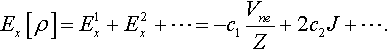
From the density scaling point of view, the first term in Eq. (18) is homogeneous of degree one, and the second term is homogeneous of degree two. This formula is consistent with our general description that any well-behaved functional can be expanded in terms of functionals homogeneous of degree 1, 2, … [24]. In addition, if one takes just the first two terms in Eq. (18) we see that Ex[ρ] thereby has been expressed as the sum of functionals homogenous of degrees one and two.
From the theoretical point of view, Eq. (18) belongs to the regime of the weighted-density approximation (WDA) [39,40], in which an energy density is expressed as a function of r and ρ(r), i.e.,
The approximations most often employed in atomic and molecular studies are the local density approximation (LDA), in which the energy density is a function of the density only, and its extension, the gradient expansion approximation and/or generalized gradient approximation (GEA/GGA), where besides the local density, the nonlocal density gradient is included in the energy density function formulation; that is,
Elsewhere [41], two of the present authors, have shown that even for the simplest hydrogen-like systems, a proper description for both the energy functional and its potential must go beyond WDA and GEA/GGA frameworks. The approximation needed takes the form
We thus anticipate that because of the rather different form Eq. (18) takes, its capability to reproduce accurate exchange energy results for many-electron atoms and molecules may be limited. Also, the exchange potential stemming from Eq. (18) is divergent at a nuclear cusp, and it does not in general decay as ![]() when r is very large. These flaws, however, do not detract from its interest as an example of constructing new approximate functionals from homogeneous functionals.
when r is very large. These flaws, however, do not detract from its interest as an example of constructing new approximate functionals from homogeneous functionals.
III Computational Methods
Neutral, positive, and negative atomic systems from H to Xe, and the Be iso-electronic series from B+ to Cr+ 20 and Ne series ions from Ne+ 1 to Ne+ 9 are investigated. A few first-row monohydrides from LiH to HF are examined as an example of the application to molecules. The restricted Hartree-Fock wavefunctions of Koga et al. [42] have been used for atomic systems. For molecules, calculations are performed at the B3PW91/6-311++G(3d, 2p) level.
Neutral atom results are used as data sets for least-square fits to determine the two constants c1 and c2. Since it is expected that Eq. (18) is not generally applicable because of its simple form, we fit the constants for every period. After the constants are determined, predictions are made for cations and anions, as well as other ionic series, the Be iso-electron series and the Ne ion series. For the molecules studied, the sum of the electrostatic potentials at the two nuclei is used, and a separate least-square fit is made.
IV Results and Discussion
Table 1 shows the exact and fitted exchange values for neutral atoms up to Z = 54. The fitted constants for each period are listed in the bottom of the table. From the table, one finds that except for the hydrogen atom, the overall relative deviation is around 1-2% for the first row, with the error becoming smaller for later rows. For example, for the fourth period, Z = 37 ~ 54, the average error is 0.06%. The relative magnitude of Ex1 and Ex2 for large atomic number atoms vary little as Z varies. For Z = 10, 18, 36, and 54, for example, Ex1 is 72, 74, 69, and 70% of the total. For Z = 2, Ex1 is 92% of the total.
Table 1
The accurate and fitted exchange energies for the first 54 neutral atoms (a.u.)
| Atom | Accurate | Fitted | Error% | Atom | Accurate | Fitted | Error% |
| 1 | -0.3125 | -0.2929 | -6.27 | 28 | -61.624 | -61.559 | -0.10 |
| 2 | -1.026 | -1.042 | 1.56 | 29 | -65.793 | -65.750 | -0.07 |
| 3 | -1.781 | -1.796 | 0.86 | 30 | -69.640 | -69.577 | -0.09 |
| 4 | -2.667 | -2.706 | 1.46 | 31 | -73.517 | -73.407 | -0.15 |
| 5 | -3.744 | -3.764 | 0.53 | 32 | -77.444 | -77.345 | -0.13 |
| 6 | -5.045 | -5.009 | -0.72 | 33 | -81.432 | -81.365 | -0.08 |
| 7 | -6.596 | -6.457 | -2.11 | 34 | -85.493 | -85.488 | -0.01 |
| 8 | -8.174 | -8.108 | -0.80 | 35 | -89.635 | -89.717 | 0.09 |
| 9 | -10.000 | -9.997 | -0.03 | 36 | -93.852 | -94.055 | 0.22 |
| 10 | -12.110 | -12.140 | 0.24 | 37 | -97.895 | -98.049 | 0.16 |
| 11 | -14.020 | -14.058 | 0.27 | 38 | -101.953 | -102.066 | 0.11 |
| 12 | -15.990 | -16.035 | 0.28 | 39 | -106.185 | -106.270 | 0.08 |
| 13 | -18.070 | -18.082 | 0.07 | 40 | -110.542 | -110.586 | 0.04 |
| 14 | -20.280 | -20.254 | -0.13 | 41 | -115.122 | -115,137 | 0.01 |
| 15 | -22.640 | -22.553 | -0.39 | 42 | -119.690 | -119.676 | -0.01 |
| 16 | -25.000 | -24.974 | -0.11 | 43 | -124.169 | -124.148 | -0.02 |
| 17 | -27.510 | -27.530 | 0.07 | 44 | -129.123 | -129.059 | -0.05 |
| 18 | -30.19 | -30.229 | 0.13 | 45 | -133.989 | -133.904 | -0.06 |
| 19 | -32.677 | -32.745 | 0.21 | 46 | -139.142 | -139.060 | -0.06 |
| 20 | -35.212 | -35.294 | 0.23 | 47 | -144.040 | -143.910 | -0.09 |
| 21 | -38.031 | -38.096 | 0.17 | 48 | -148.916 | -148.814 | -0.07 |
| 22 | -40.993 | -41.039 | 0.11 | 49 | -153.826 | -153.713 | -0.07 |
| 23 | -44.089 | -44.116 | 0.06 | 50 | -158.780 | -158.689 | -0.06 |
| 24 | -47.489 | -47.505 | 0.03 | 51 | -163.766 | -163.738 | -0.02 |
| 25 | -50.686 | -50.681 | -0,01 | 52 | -168.825 | -168.862 | 0.02 |
| 26 | -54.190 | -54.162 | -0.05 | 53 | -173.924 | -174.062 | 0.08 |
| 27 | -57.835 | -57.790 | -0.08 | 54 | -179.092 | -179.337 | 0.14 |

The fitted parameters for 
(i). C1 = -0.27615 and C2 = -0.053636 for Z = 1 - 10;
(ii). C1 = -0.31864 and C2 = -0.034591 for Z = 11 - 18;
(iii). C1 = -0.34814 and C2 = -0.02593 for Z = 19 - 36;
(iv). C1 = -0.39475 and C2 = -0.01870 for Z = 37 - 54.
The large error found in the hydrogen atom case presumably results from the discrepancy between Eq. (18) and the correct formalism for the hydrogen-like system [41]. For the one-electron atomic system, the classical interelectron repulsion should cancel the total exchange energy [43,44], i.e.,
so that there is no net two-electron interaction energy. This requirement is not satisfied in Eq. (18), in which Ex depends on both Vne/Z and J for atoms.
In Tables 2 and 3, predictions are made of exchange energies for the first positive and negative ions of atoms, respectively. Good agreement with the accurate values is found. The general tendency and the average error percentage of these predictions are about the same as those of Table 1 on which the least square fits were made. The forth row of elements generates the best data. The average error of this row in Table 3 is just 0.09%, and in Table 2, 0.13%.
Table 2
Predicted exchange energies for the first cation of the first 54 elements (a.u.).
| Cation | Accurate | Predict | Error% | Cation | Accurate | Predict | Error% |
| 2 | -0.625 | -0.5858 | -6.27 | 29 | -65.063 | -64.816 | -0.38 |
| 3 | -1.652 | -1.662 | 0.57 | 30 | -69.511 | -69.197 | -0.45 |
| 4 | -2.507 | -2.515 | 0.31 | 31 | -73.344 | -73.065 | -0.38 |
| 5 | -3.492 | -3.531 | 1.11 | 32 | -77.242 | -76.952 | -0.36 |
| 6 | -4.712 | -4.710 | -0.03 | 33 | -81.201 | -80.936 | -0.33 |
| 7 | -6.124 | -6.083 | -0.67 | 34 | -85.227 | -85.022 | -0.24 |
| 8 | -7.739 | -7.665 | -0.96 | 35 | -89.332 | -89.208 | -0.14 |
| 9 | -9.566 | -9.474 | -0.96 | 36 | -93.109 | -93.504 | 0.43 |
| 10 | -11.617 | -11.527 | -0.77 | 37 | -97.812 | -97.832 | 0.02 |
| 11 | -13.902 | -13.866 | -0.26 | 38 | -101.86 | -101.820 | -0.04 |
| 12 | -15.863 | -15.804 | -0.37 | 39 | -105.93 | -105.878 | -0.05 |
| 13 | -17.893 | -17.855 | -0.21 | 40 | -110.25 | -110.164 | -0.08 |
| 14 | -20.045 | -19.982 | -0.31 | 41 | -114.67 | -114.552 | -0.10 |
| 15 | -22.307 | -22.232 | -0.34 | 42 | -119.42 | -119.227 | -0.16 |
| 16 | -24.687 | -24.610 | -0.31 | 43 | -124.06 | -123.834 | -0.18 |
| 17 | -27.075 | -27.121 | 0.17 | 44 | -128.53 | -128.329 | -0.16 |
| 18 | -29.820 | -29.766 | -0.18 | 45 | -133.65 | -133.356 | -0.22 |
| 19 | -32.294 | -32.565 | 0.84 | 46 | -138.58 | -138.274 | -0.22 |
| 20 | -35.108 | -35.086 | -0.06 | 47 | -143.95 | -143.548 | -0.28 |
| 21 | -37.673 | -37.685 | 0.03 | 48 | -148.78 | -148.426 | -0.24 |
| 22 | -40.621 | -40.596 | -0.06 | 49 | -153.66 | -153.363 | -0.19 |
| 23 | -43.703 | -43.639 | -0.15 | 50 | -158.59 | -158.307 | -0.18 |
| 24 | -46.917 | -46.816 | -0.21 | 51 | -163.56 | -163.324 | -0.14 |
| 25 | -50.572 | -50.377 | -0.38 | 52 | -168.58 | -168.416 | -0.10 |
| 26 | -53.752 | -53.584 | -0.31 | 53 | -173.66 | -173.582 | -0.04 |
| 27 | -57.379 | -57.181 | -0.34 | 54 | -178.81 | -178.825 | 0.01 |
| 28 | -61.149 | -60.924 | -0.37 | 55 | -184.02 | -184.147 | 0.07 |

Parameter values from Table 1.
Table 3
Predicted exchange energies for the first anion of the first 54 elements (a.u.).
| Anion | Accurate | Predict | Error% | Anion | Accurate | Predict | Error% |
| 1 | -0.3955 | -0.421 | 6.48 | 28 | -61.899 | -62.007 | 0.17 |
| 3 | -1.827 | -1.867 | 2.17 | 29 | -65.846 | -65.964 | 0.18 |
| 5 | -3.843 | -3.899 | 1.46 | 31 | -73.595 | -73.614 | 0.03 |
| 6 | -5.150 | -5.205 | 1.06 | 32 | -77.564 | -77.610 | 0.06 |
| 7 | -6.648 | -6.712 | 0.97 | 33 | -81.587 | -81.689 | 0.12 |
| 8 | -8.352 | -8.443 | 1.08 | 34 | -86.200 | -85.864 | -0.39 |
| 9 | -10.274 | -10.412 | 1.35 | 35 | -89.852 | -90.143 | 0.32 |
| 11 | -14.062 | -14.162 | 0.71 | 37 | -97.925 | -98.171 | 0.25 |
| 13 | -18.150 | -18.221 | 0.39 | 39 | -106.32 | -106.517 | 0.19 |
| 14 | -20.373 | -20.444 | 0.35 | 40 | -110.71 | -110.871 | 0.15 |
| 15 | -22.711 | -22.788 | 0.34 | 41 | -115.17 | -115.322 | 0.13 |
| 16 | -25.168 | -25.262 | 0.37 | 42 | -119.74 | -119.870 | 0.12 |
| 17 | -27.749 | -27.871 | 0.44 | 43 | -124.38 | -124.520 | 0.11 |
| 19 | -32.715 | -32.846 | 0.40 | 44 | -129.17 | -129.271 | 0.08 |
| 21 | -38.203 | -38.347 | 0.38 | 45 | -134.00 | -134.123 | 0.09 |
| 22 | -41.173 | -41.310 | 0.33 | 46 | -139.01 | -139.080 | 0.05 |
| 23 | -44.283 | -44.414 | 0.29 | 47 | -144.09 | -144.143 | 0.04 |
| 24 | -47.535 | -47.650 | 0.24 | 49 | -153.91 | -153.942 | 0.02 |
| 25 | -50.917 | -51.025 | 0.21 | 50 | -158.89 | -158.974 | 0.05 |
| 26 | -54.436 | -54.539 | 0.19 | 51 | -163.92 | -164.068 | 0.09 |
| 27 | -58.095 | -58.200 | 0.18 | 52 | -168.99 | -169.232 | 0.14 |
| 53 | -174.13 | -174.469 | 0.19 |

Parameter values from Table 1.
Another example showing that Eq. (18) produces good results for heavy atoms is exhibited in Table 4, where accurate and predicted exchange energies for the Be iso-electron series are given. The estimated results are calculated by using the constants of the first-row fit. One sees that as the atomic charges Z increases from B +, the error percentage decreases from 1.11% to 0.13%. The larger the atomic number, the more accurate the estimated result.
Table 4
Predicted exchange energies for the Be-isoelectronic series from B to Cr (a.u.).
| Accurate | Predict | Error% | |
| B+ | -3.492 | -3.531 | 1.11 |
| C+ 2 | -4.314 | -4.352 | 0.88 |
| N+ 3 | -5.135 | -5.172 | 0.72 |
| O+ 4 | -5.956 | -5.992 | 0.61 |
| F+ 5 | -6.776 | -6.811 | 0.52 |
| Ne+ 6 | -7.596 | -7.630 | 0.45 |
| Na+ 7 | -8.415 | -8.449 | 0.41 |
| Mg+ 8 | -9.235 | -9.268 | 0.36 |
| Al+ 9 | -10.054 | -10.09 | 0.33 |
| Si+ 10 | -10.874 | -10.906 | 0.29 |
| P+ 11 | -11.693 | -11.725 | 0.27 |
| S+ 12 | -12.513 | -12.543 | 0.24 |
| Cl+ 13 | -13.332 | -13.362 | 0.23 |
| Ar+ 14 | -14.152 | -14.182 | 0.20 |
| K+ 15 | -14.971 | -14.999 | 0.19 |
| Ca+ 16 | -15.79 | -15.818 | 0.18 |
| Sc+ 17 | -16.61 | -16.637 | 0.16 |
| Ti+ 18 | -17.429 | -17.455 | 0.15 |
| V+ 19 | -18.248 | -18.275 | 0.15 |
| Cr+ 20 | -19.068 | -19.093 | 0.13 |

Evaluated using c1 = -0.27615 and c2 = -0.0053626. See Table 1 and text.
Table 5 shows the accurate and predicted exchange energy results for the Ne positive ions series. Except for the one-electron Ne+ 9 cation, one finds the relative error is less than 2% for each species, falling in the same range of error as the first-row species in Table 1.
Table 5
The accurate and predicted exchange energies for the Ne cation series (a.u.).
| Accurate | Predict | Error% | |
| Ne+ 9 | -3.125 | -2.929 | -6.27 |
| Ne+ 8 | -6.028 | -5.997 | -0.52 |
| Ne+ 7 | -6.843 | -6.808 | -0.52 |
| Ne+ 6 | -7.596 | -7.630 | 0.45 |
| Ne+ 5 | -8.552 | -8.467 | -0.99 |
| Ne+ 4 | -9.446 | -9.290 | -1.65 |
| Ne+ 3 | -10.265 | -10.084 | -1.77 |
| Ne+ 2 | -10.994 | -10.835 | -1.44 |
| Ne+ 1 | -11.617 | -11.527 | -0.77 |

To test the more general applicability of Eq. (18), we have investigated a few molecular species. Table 6 shows the ab initio and estimated results for the first-row mono hydrides. Ab initio results are obtained at the B3PW91/6-311++G(3d, 2p) level with the optimized geometry. The quantities computed include the classical Coulomb repulsion energy J, the electrostatic potential at each nucleus Vne1 and Vne2, and the exchange energy from the B3PW91 functional. Then, a least-square fit is performed to determine the constants c1 and c2 in Eq. (18) for this set of molecules. The absolute error of the fitted results is less than 0.02 a.u., the relative error around 1% or less. Equation (18) is a good approxiation for molecular systems.
Table 6
The approximated density functional and fitted exchange energies for a few first-row monohydrides. The calculated data were obtained at the B3PW91/6-311++G (3df, 2p) level. See text.
| Mols. | J | Vnel* | Vne2* | Ex | |
| DFT | Fitted (Error %)** | ||||
| LiH | 5.192 | 2.235 | 6.073 | -1.685 | -1.704 (1.10) |
| BeH | 8.544 | 2.741 | 8.807 | -2.421 | -2.428 (0.30) |
| BH | 13.284 | 3.269 | 11.830 | -3.260 | -3.271 (0.33) |
| CH | 19.917 | 3.894 | 15.191 | -4.290 | -4.276 (-0.32) |
| NH | 28.664 | 4.582 | 18.864 | -5.454 | -5.444 (-0.18) |
| OH | 39.872 | 5.324 | 22.885 | -6.814 | -6.795 (-0.28) |
| FH | 53.834 | 6.112 | 27.216 | -8.315 | -8.334 (0.22) |

* Vne1 is defined as the electrostatic potential 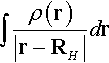 at the hydrogen nucleus, and Vne2 is defined as the electrostatic potential
  at the other atom.
** The fitted formula for this series of molecules is:
![]()
V Summary
To illustrate the argument that any well-behaved functional can be expressed as the sum of density-homogeneous functionals, starting from the Levy-Perdew relation, we have shown that the exchange energy density functional can be written, at least approximately, as the sum of functionals homogeneous of degree one and two, respectively, with respect to the density scaling. This formula is consistent with the recent suggestion that the functional Vee[ρ], of which Ex[ρ] is a part, has a truncated functional expansion and can be expressed as a combination of density homogeneous functionals of degrees one and two. Though an approximation, the formulation gives good estimation of the exchange energy for both atoms and ions, especially for large systems. Extension to simple molecules, the first-row monohydrides, also gives good fits.
Acknowledgment
This work has been supported by National Science Foundation, the Petroleum Research Fund of the American Chemical Society, the North Carolina Supercomputing Center, and the Hungarian-U.S. Science and Technology Joint Fund. SBL thanks Professor Jan Hermans for partial support from a Research Resource project in computational structural biology (NIH grant RR08102). FDP is a postdoctoral fellow of the Fund for Scientific Research-Flanders (Belgium) and also has been supported by Fulbright and NATO travel grants enabling a stay at the University of North Carolina. RGP acknowledges with pleasure the steady friendship, over many years, both professional and personal, of Giuseppe Del Re. Professor Del Re is a theoretical chemist with firm conviction, often eloquently expressed, that the understanding of molecular electronic structure demands careful mathematical analysis as well as computation, and both deep and earnest thought.