The first attempt to determine the HPHF orbitals was analogous to the procedure used initially for the PHF orbitals [5]. For this purpose, the Brillouin procedure was extended to the PHF scheme. Two sets of occupied orbitals, each of them associated with different spin functions, are written in terms of a limited basis:

$\begin{array}{l}{a}^1,a^2,\dots ,a^p,\dots ,a^{n/2}\\ b^1,b^2,\dots ,b^p,\dots ,b^{n/2}\end{array}$

In the same way, the virtual orbitals corresponding to the complementary space can be expressed as:

$\begin{array}{l}{a}^{\left(n/2\right)+1},\dots ,a^t,\dots ,a^m\\ a^{\left(n/2\right)+1},\dots ,b^t,\dots ,b^m\end{array}$

The trial occupied orbitals are then corrected in terms of the virtual ones:

$\begin{array}{l}{a}^p=a_o^p+{\displaystyle \sum _{\mathrm{t}=\left(n/2\right)+1}^m{c}_{\mathit{pt}}{a}_o^t}\\ b^p=b_o^p+{\displaystyle \sum _{\mathrm{t}=\left(n/2\right)+1}^m{c}_{\mathit{pt}}^{\prime }{b}_o^t}\end{array}$

and introduced in the PHF function which is developed in terms of single, double, triple,…, excitations.

$\mathrm{\Psi }={\mathrm{\Psi }}_o+{\displaystyle \sum _{\mathit{pt}}{c}_{\mathit{pt}}}{\mathrm{\Psi }}_o^{\mathit{pt}}+{\displaystyle \sum _{\mathit{pt}}{c}_{\mathit{pt}}^{\prime }\mathit{Ps}{i}_o^{p^{\prime }{t}^{\prime }}}+{\displaystyle \sum _{\mathit{pt},\mathit{qv}}{c}_{\mathit{pt}}{c}_{\mathit{qv}}^{\prime }{\mathrm{\Psi }}_o^{\mathit{pt},q^{\prime }{v}^{\prime }}}+\dots$

where Ψ_o^pt are the Slater determinants in which an occupied orbital, a^p, has been replaced by a virtual one, a^t, and so on. The corrections c_pt and c′_pt are then determined by minimizing the total energy.

The conditions which minimize the energy are obtained by setting the partial derivatives with respect to the corrections equal to zero:

$\begin{array}{c}0=<{\mathrm{\Psi }}_o^{\mathit{pt}}|H-E|{\mathrm{\Psi }}_o>+{\displaystyle \sum _{\mathit{qv}}{c}_{\mathit{qv}}[<}{\mathrm{\Psi }}_o^{\mathit{pt},\mathit{qv}}|H-E|{\mathrm{\Psi }}_o>+<{\mathrm{\Psi }}_o^{\mathit{pt}}|H-E|{\mathrm{\Psi }}_o^{\mathit{qv}}>]\\ +{\displaystyle \sum _{\mathit{qv}}{c}_{\mathit{qv}}^{\prime }}\left[<{\mathrm{\Psi }}_o^{\mathit{pt},q^{\prime }{v}^{\prime }}|H-E|{\mathrm{\Psi }}_o>+<{\mathrm{\Psi }}_o^{\mathit{pt}}|H-E|{\mathrm{\Psi }}_o^{q^{\prime }{v}^{\prime }}>\right]\\ +\mathit{higher}\mathit{order}\mathit{terms}\end{array}$

There are as many equations as corrections. These equations are not linear. Their solutions would yield the exact PHF orbitals in the functional space of dimension m, but they are unmanageable.

However, whenever the starting orbitals, a_o^p and b_o^p, are sufficiently close to the solutions, the terms of second and higher order in the corrections may be neglected in (14). As a result, the conditions (14) become linear and nonhomogeneous. The solution of this system will provide new improved orbitals, that may be used to start an iterative process. When selfconsistency is reached, the corrections are zero. The conditions (14) take the form:

$0=<{\mathrm{\Psi }}^{\mathit{pt}}|H-E|\mathrm{\Psi }>\mathrm{and}0=<{\mathrm{\Psi }}^{p^{\prime }{t}^{\prime }}|H-E|\mathrm{\Psi }>$

These requirements on the matrix elements are precisely the generalized Brillouin conditions for the PHF functions [5]. They are very general and hold also for all the DODS type funtions such as the HPHF function, as well as for the RHF function.

2.2 The Pairing Theorem

Since the HPHF function is invariant under an unitary transformation applied to the orbitals a_i or/and b_i, both sets may be conveniently transformed so that the orbitals belonging to different electron pairs are orthogonal:

$〈a_i\left|b_j\right.〉={\lambda }_i{\delta }_{\mathit{ij}}$

Such orbitals are known as corresponding orbitals [4].

As a result, the overlap between the HPHF function with itself may be expressed as:

$〈{\mathrm{\Psi }}^{\mathit{HPHF}}|{\mathrm{\Psi }}^{\mathit{HPHF}}〉=1+D$

where:

$D={\displaystyle \prod _{i=1}^n{\lambda }_i^2}$

2.3 The HPHF Equations

In order to deal with the HPHF equations, it is convenient to define a series of operators analogous to those of the UHF model:

$\begin{array}{l}{\widehat{F}}^a=\widehat{h}+\widehat{J}\left({\widehat{R}}^a+{\widehat{R}}^b\right)-\widehat{K}{\widehat{R}}^a\\ {\widehat{F}}^b=\widehat{h}+\widehat{J}\left({\widehat{R}}^a+{\widehat{R}}^b\right)-\widehat{K}{\widehat{R}}^b\\ {\widehat{F}}^{\mathit{ab}}=\widehat{h}+2\widehat{J}\left({{\widehat{R}}^a}^b\right)-\widehat{K}{\widehat{R}}^{\mathit{ab}}\end{array}$

In these expressions, $\widehat{h}$, $\widehat{J}$ and $\widehat{K}$ are the usual monoelectronic coulombic, bielectronic coulombic and exchange operators, respectively. ${\widehat{R}}^a$ and ${\widehat{R}}^b$ are the one-particle density operators expressed in the a_i and b_i orbital basis:

$\begin{array}{l}{\widehat{R}}^a={\displaystyle \sum _{i=1}^n\left|a_i\right.〉}\left.〈a_i\right|\\ {\widehat{R}}^b={\displaystyle \sum _{i=1}^n\left|b_1\right.〉}\left.〈b_i\right|\end{array}$

In the same way, ${\widehat{R}}^{\mathit{ab}}$ is a cross density operator between both basis sets:

${\widehat{R}}^{\mathit{ab}}={\displaystyle \sum _{i=1}^n\frac{\left|a_i\right.〉\left.〈b_i\right|}{{\lambda }_i}}$

With these definitions, the total HPHF electronic energy may be easily written down:

$E_{\mathit{HPHF}}=\frac{E_{\mathit{UHF}}+E_{\mathit{cross}}}{1+D}$

where E_UHF should be the one-DODS-determinant energy and E_cross, the interaction energy between both determinants:

$\begin{array}{l}{E}_{\mathit{UHF}}=\frac{1}{2}\mathit{Tr}\left[\left({\widehat{R}}^a+{\widehat{R}}^b\right)\widehat{h}+{\widehat{R}}^a{\widehat{F}}^a+{\widehat{R}}^b{\widehat{F}}^b\right]\\ E_{\mathit{cross}}=\mathit{DTr}\left[{\widehat{R}}^{\mathit{ab}}\widehat{h}+{\widehat{R}}^{a}b{\widehat{F}}^{\mathit{ba}}\right]\end{array}$

From the energy expression for the HPHF function (23), the pseudoeigen-value equations for the HPHF orbitals may be easily deduced resorting to the Generalized Brillouin Theorem expression [10]. This theorem has been shown to be valid for any MCSCF function [17] and, in particular, for a two determinant SCF function [7,8]:

$\frac{\partial E}{\partial C_{\mathit{it}}}=〈\mathrm{\Psi }|H-E|{\mathrm{\Psi }}^{\mathit{it}}〉=0$

where Ψ is now the HPHF function for the singlet ground state and is Ψ^it a HPHF function in which an a_i occupied orbital has been replaced by a virtual one a_t.

This expression may be rewritten in terms of the two DODS functions and, taking into account the idempotency of the operator $\widehat{A}\left(S\right)$ (9):

$\frac{\partial E}{\partial C_{\mathit{it}}}=〈{\mathrm{\Psi }}_o\left|\widehat{H}\right|\left({\mathrm{\Psi }}_o^{\mathit{it}}+{\mathrm{\Psi }}_n^{\mathit{it}}\right)〉-〈{\mathrm{\Psi }}_o|\left({\mathrm{\Psi }}_o^{\mathit{it}}+{\mathrm{\Psi }}_n^{\mathit{it}}\right)〉$

Developing this last expression in terms of the corresponding orbitals, we have

$\begin{array}{c}〈a_i\left|{\widehat{F}}^a\right|a_t〉+\frac{1}{{\lambda }_i}〈b_i|a_t〉\left(E_{\mathit{cross}}-\mathit{DE}\right)+\\ +\frac{D}{{\lambda }_i}〈b_i\left|{\widehat{F}}^{a}b\right|a_t〉-\frac{D}{{\lambda }_i}{\displaystyle \sum _j^n\frac{1}{{\lambda }_j}〈b_j|a_j〉〈b_i\left|{\widehat{F}}^{\mathit{ba}}\right|a_j〉}=0\end{array}$

We can now express this equation in compact form as:

$〈a_i\left|H^a\right|a_t〉=0$

A similar equation may be written for the b_i orbitals.

Since Ψ^HPHF is invariant under an unitary transformation, two canonical sets of a_i and b_i, which diagonalize the matrix representation of ${\widehat{H}}^a$ and ${\widehat{H}}^b$ operators, may be chosen:

$\begin{array}{c}{\widehat{H}}^a\left|a_i\right.〉={\epsilon }_i^a\left|a_i\right.〉\\ {\widehat{H}}^b\left|b_i\right.〉={\epsilon }_i^b\left|b_i\right.〉\end{array}$

The expression (26) was developed in Ref. [10], and it is possible to show that it is equivalent to the diagonal of expression given by Smeyers et al. [11,18].

In matrix form, expression (26) may be rewritten as:

$\begin{array}{c}{\mathbf{H}}^{\mathbf{a}}={\mathbf{F}}^{\mathbf{a}}+\mathbf{S}\left({\mathbf{R}}^{\mathbf{ab}}\mathbf{+}{\mathbf{R}}^{\mathbf{ba}}\right)\mathbf{S}\left(E_{\mathit{cross}}-\mathit{DE}\right)+\\ +D\left\{\mathbf{S}{\mathbf{R}}^{\mathbf{ab}}{\mathbf{F}}^{\mathbf{ba}}\left[\mathbf{I}-{\mathbf{R}}^{\mathbf{ab}}\mathbf{S}\right]+\left[\mathbf{I}-\mathbf{S}{\mathbf{R}}^{\mathbf{ba}}\right]{\mathbf{F}}^{\mathbf{ab}}{\mathbf{R}}^{\mathbf{ba}}\mathbf{S}\right\}\end{array}$

where S is the overlap matrix between the basis functions used for expanding the orbitals.

The procedure is carried out by diagonalizing the H^a and H^b matrices in an alternated way just as in the UHF procedure until the convergence is reached.

2.4 Some Applications to Singlet Ground States

Because of the complexity of the PHF function, only very small electronic systems were initially considered. As first example, the electronic energy of some four electron atomic systems was calculated using the Brillouin procedure [8]. For this purpose, a short double zeta STO basis set, 1 s, 1 s’, 2 s and 2 s’, with optimized exponents was used. The energy values obtained are given in Table 1. In the same table, the RHF energy values calculated with the same basis are gathered for comparison. It is seen that the PHF model introduces some electronic correlation in the wave-function. Because of the nature of the basis set formed by only s-type orbitals, only radial correlation is included which account for about 30% of the electronic correlation energy.

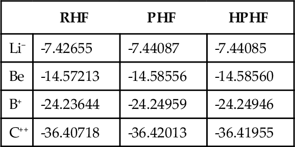
In the same table, the HPHF energy for the same systems obtained with the same basis are also given. It is seen that the HPHF model furnishes energy values very close to the PHF ones with much less work and less computation time.

The HPHF potential energy curve calculated as a function of the nuclear separation in lithium hydride is given in Figure 1. Six STO’s as basis functions, 1 s, 1 s’, 2 s, 2p_σ, on the Li atom, and 1 s and 2p_σ on the H atom, with adjustable exponents, were used. In the same figure, the RHF potential energy curve obtained in the same conditions is also represented. It is seen that the HPHF curve dissociates correctly into neutral atoms, whereas the RHF ones does it incorrectly into ions. The HPHF model is seen to introduce some alternant correlation effects in the wave-function.

It is interesting to point out that models such as the PHF and HPHF ones, which resort to orthogonal projection are able to open only one electronic shell, i.e., they are able to introduce either radial or alternant correlation [19]. This is the limitation of these models. To introduce simultaneouly both effects non-orthogonal projection operadors have to be used [20].

In an attempt to check the performance of the HPHF model for determining singlet excited states, most of the excited states of the lithium molecule, L12, were determined as a function of the nuclear separation, and their spectroscopic constants evaluated. In this aim, the standard 6-311G* basis set was used for all of them [15].

In Fig.2, the corresponding potential curves are represented, including that of the C¹Σ_g⁺ state with identical symmetry as that of the ground state.

In this table it is seen that the values obtained in the HPHF approach for the spectroscopic constants of Li₂ in its first singlet excited state are especially satisfactory when compared with the MCSCF and experimental values. The values for higher excited states are not so good, probably because of the contamination of higher spin states, as well as the use of a basis set built up essentially for the ground state. Finally, it is noticeable that the values found for the ground state are not satisfactory at all, this result is generally observed when using DODS functions, which rise to a too flat potential energy curve.

4.2 Cyclobutanone and Cyclopentenone in their first singlet excited states

As a test for checking the effectiveness of the model, we have applied the procedure and determined the optimal geometries of two relatively large molecules: cyclobutanone and 3-cyclopenten-l-one [16], which are well known in their first (n → π*) excited state [23–26].

To optimize the geometry, we used the Simplex method recently implemented into the HPHF program [27].

4.3 Core excitations

Finally, the applications of the Half-Projected-Hartree-Fock model have not to be limited to the excitations of the valence electron shell. This model can also be used to study core electron excitations. This aspect is especially interesting, since there are very few efficient methods for such calculations in molecular systems [29,30].

In order to illustate this possibility, the SF₆ molecule, for which there exist experimental data has been tested [31]. For this purpose different basis sets for the different excitations have to be used. For 1 s excitations in the central sulfur atom, the standard chlorine atom basis was employed for describing all the sulfur electrons. For the 2 s or 2p excitations in the same atom, the chlorine atom basis was employed for describing the sulfur L and M shells. The corresponding excitation values are given in Table 4.

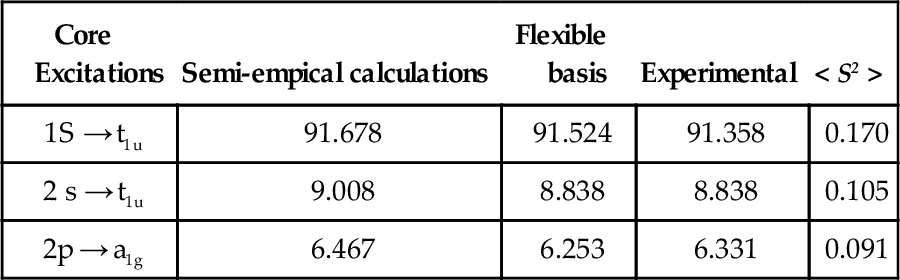
It is seen that the HPHF model reproduces satisfactorily the core excitations in SF₆, even better than some semi-empirical procedures [32]. The mean total spin momentum values are seen also to be very small.