Appendices
| A Performance Degradation Because of Rain |
| B QPSK Modulation and Demodulation |
| C Algebraic Preliminaries |
| D BCH Code Details |
| E Cyclical Redundancy Code |
| F AS Matrix |
| G Operators, Mnemonics, Abbreviations |
Appendix A. Performance Degradation Because of Rain
For carrier frequencies above 10 GHz, rain will degrade performance. The following three different mechanisms contribute to this degradation.
1. Attenuation
2. An increase in sky noise temperature
3. Interference from adjacent channels when polarization is used for frequency reuse. This is caused by depolarization.
Each of these sources of degradation is calculated in the sections here, followed by a discussion of how each affects performance.
A.1 Rain Attenuation
Of particular interest for a DBS system is the percentage of time that certain values of attenuation are exceeded. The total attenuation is defined as
(A.1)
![]()
where αp equals the specific attenuation in dB per km, and L equals the effective path length in km.
The specific attenuation is defined as
(A.2)
![]()
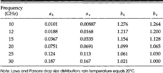
where a and b depend on the frequency and the polarization. The parameters a and b for linear polarization are tabulated as a function of frequency.
The a and b parameters for circular polarization can then be calculated from their linear counterparts. Table A.1 gives the values for a and b as a function of frequency.
Table A.1 Specific Attenuation Coefficients for Rain Attenuation Calculations
Rp is the rain rate in mm per hour and the effective path length L is equal to the rain slant length multiplied by a reduction factor rp or L = Ls * rp. The subscript p in each case refers to the fraction of a year that the parameter is exceeded.
These can all be combined to form the complete expression for rain attenuation:
(A.3)
![]()
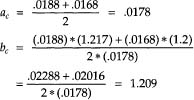
For DBS the downlink frequency is approximately 13 Ghz, so from Table A.1, ah = .0188, av = .0168, bh = 1.217, bv = 1.2. For circular polarization,

The a and b parameters for circular polarization can be calculated as follows:
(A.4)
![]()
Taking into account the Earth’s curvature,
(A.5)
![]()
where

In the continental United States, φ ranges from 24.5° to 49° and θ from 27° to 54°. Therefore, c ranges from .69 to 1.0. For c = .69,

For the larger φ,
![]()
For the purposes of obtaining some numerical results, assume the calculation for close to sea level (ho = .2 km) and use Equation (A.5).
(A.6)
![]()
For the lower lattitudes, using hR = 3.18 km and θ = 54°, we have
(A.7)
![]()
For the higher lattitudes, using hR = 1.915 km and θ = 27°, we have
(A.8)
![]()
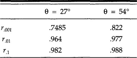
Next, rp can be determined from Table A.2. For r001,
Table A.2 Slant Range Reduction Factor
![]()
Forr.01,
![]()
Forr.1,
![]()
where LG = Ls * cos0. For 6 = 54°, LG = 3.68 * cos[54°] = 2.16 km, while forθ = 27°, LG = 3.77 * cos [27°] = 3.36 km.
Finally, we can calculate the total attenuation for θ = 27° and θ = 54°. For θ = 27°,
![]()
![]()
Forθ = 27°,
(A.9)
![]()
Forθ = 54°,
(A.10)
![]()
Examination of Equations (A.9) and (A.10) shows that the attenuation in the United States is almost entirely determined by Rp.
Referring to the Region 2 rain zone map (Figure A.1) and rain rate distribution (see Table A.3), the United States ranges from a Region B to a Region M. If we consider a good quality of service, such as .1 percent outage per year (8.76 hours), we obtain
(A.11)
![]()
Figure A.1 Region 2 Rain Model
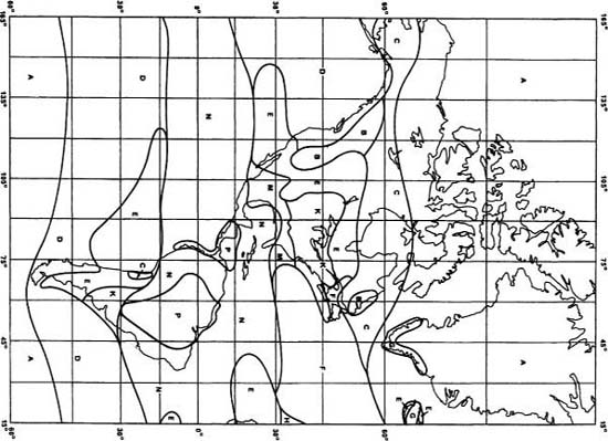
Table A.3 Rain Rate Distributions for the Rain Climate Zones of the CCIR Prediction Model
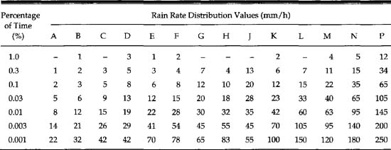
Using R.1 = 2, we have A.1 = .152 dB. Thus, the attenuation is negligible. Next, however, consider Region M,
![]()
Thus, we see one of the reasons the margins are set high.
A.2 The Effect of Rain on System Noise Temperature
In addition to the attenuation of the signal power because of the rain, rain also increases the system noise temperature. This lowers G/T, further decreasing the carrier-to-noise (C/N). The increase in noise temperature is
![]()
where Tr is normally taken to be 273°K. In the previous example,

Since G/T was 11.39 dB/°K, with Ts = 125 K,
![]()
Thus, the rain has caused another 3 dB drop in the C/N.
A.3 Adjacent Channel Interference and Depolarization Effects Due to Rain
Adjacent channels are separated by 14.28 Mhz (see Figure 2.1). These channels are isolated by the fact that they have opposite polarization (right-hand circular or left-hand circular). With clear sky conditions, this isolation is 26 dB and does not significantly affect the C/N. However, rain causes a depolarization that creates adjacent channel interference.
Appendix B shows that QPSK can be considered to be the sum of two independent BPSK modulation paths, each operating at a bit rate equal to the QPSK symbol rate. Referring to Figure B.1, each path consists of the digital signal being passed through a transmit low-pass filter, multiplied by a sinusoid, and then output summation. The multiplication by the sinusoid translates the Power Spectral Density (PSD) in frequency but does not change its shape. Likewise, the summation does not change the shape of the Power Spectral Density. Thus, we can concentrate on the PSD of the digital signal and its modification by the transmit low-pass filter.
First, it can be shown [Ha90, Appendix 9B]1 that the PSD for bipolar signaling is
1 Ha, Tri. Digital Satellite Communications. New York: McGraw Hill, 1990.
![]()
where c is a constant, and Ts is the symbol period. For the major DBS systems, Ts = 50 * 10-9 seconds. In this expression for s(f),f= 0 corresponds to the carrier frequency. Figure A.2 is a plot of s(f).
Figure A.2 Bipolar Power Spectral Density
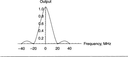
Because the transponder bandwidth is only 24 Mhz, and the transponder centers only 29 Mhz, it is clear that the output of the bipolar signal needs to be band-pass filtered. To see this, look at the value of the output at 14.5 MHz on either side of 0 in Figure A.2. The output hasn’t even reached the first null. Thus, there is main-lobe energy and all the side-lobe energy in the adjacent transponders.
A raised cosine filter is defined by

The parameters f1 and B are defined by a parameter called the roll-off factor ρ, 0 ≤ ρ ≤ 1, as

For the major DBS systems, p is chosen to be .35. Because Rsymbol = 20 * 106 symbols/sec,

and
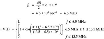
Figure A.3 shows V(f). The Power Spectral Density of the filter output is
Figure A.3 Raised Cosine Filter

![]()
Therefore,

Figure A.4 shows this output PSD. It should be noted that V(f) is a band-pass filter that is symmetric in negative frequency. The power in-band (in arbitrary units) is
Figure A.4 Output Power Spectral Density


With this filtering, there is negligible adjacent channel interference from the same polarization. However, the adjacent channel of the opposite polarization will interfere when it is depolarized by rain.
Plotted on Figure A.4, it would be centered at 14.58 MHz and would be the curve of Figure A.4 translated to the right by 14.58 MHz. Its power, in the in-band (the interfering power), is
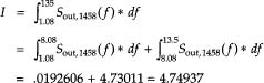
This is the power from the adjacent opposite polarization band. It is lowered by the cross-polarization discrimination before it becomes in-band interference.
The cross-polarization discrimination, XPD, is an empirically determined value,
![]()
where
![]()
and
![]()
where τ = tilt angle of polarization with respect to horizontal; τ = 45° for circular polarization, and θ = elevation angle. Using θ = 45°,
![]()
Thus, for DBS,
![]()
For clear sky conditions, Ap = 1 and XPD = 26 dB. The effective adjacent cross-polarization band power is reduced by this amount to .0119, which is negligible.
However, when there is rain, Ap > 1 and the XPD is reduced. From the example earlier in this section, A.1 = 1.86 = 2.69 dB and

Because there are interfering transponders on both sides, the total relative interfering power is 2(4.74937)/100 = .095. In this example then,
![]()
A.4 Total Effects from Rain
We are now in a position to calculate the total effects of rain on the signal-to-noise:
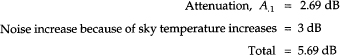
Thus, the clear sky C/N of 13 dB has been reduced to
C/N = 7.31 dB
which is still above threshold, but getting close. The total carrier-to-noise plus interference ratio is given by

Therefore, C/η is still above threshold. Thus, the system should work more than 99.9 percent of the time.