Appendix D. BCH Code Details

D.1 Generator Polynomial

The generator polynomial of this code is specified in terms of its roots from the Galois field GF(2^m) [Lin+83].¹ Let α be a primitive element in GF(2^m). The generator polynomial g(x) of the t- error correcting BCH code of length 2^m – 1 is the lowest-degree polynomial over GF(2), which has as its roots:

Lin, Shu, and Daniel J. Costello, Jr., Error Control Coding Fundamentals and Applications. New York: Prentice-Hall, 1983.

(D.1)

Thus, g(x) has α, α², α³,…, α^2t and their conjugates as all its roots. If φ_i(x) is the minimal polynomial of α_i, then g(x) is the least common multiple of α(x), φ₁(x),φ₂(x),…,φ_2t(x), that is,

(D.2)

It can be shown that the even power of a, has the same minimum polynomial as some preceding odd power of a in the sequence, and is redundant. Thus, Equation (D.2) can be reduced to

(D.3)

Since there are t of these minimal polynomials, each of degree ≤m, the degree of g(x) is less than or equal to mt.

Definition: a binary n-tuple

is a code word if and only if

(D.4)

If v(x) has roots from GF(2), α, α²,…, α^2t, it follows that v(x) is divisible by the minimal polynomials φ₁(x), φ₂(x), φ_2t(x) of d, d²,…, d^2t and, hence, by the LCM of the φ_i(x), g(x). Let

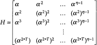
be a code polynomial in a t-error-correcting BCH code of length n = 2^m - 1 Since αⁱ is a root of v(x), 1 ≤ i ≤ 2t, then

This can be written in matrix form as

(D.5)

Next, we can form the matrix

(D.6)

Thus, the code is the null space of the matrix H, and H is the parity-check matrix of the code. The matrix H can be reduced so that the basic entries are odd powers of α.

It can be shown [Lin+83] that the minimum weight of the t-error-correcting code just defined is at least 2t + 1. Thus, the minimum distance of the code is at least 2t + 1, which is called the designed distance of the code. The true distance of a particular code may be equal to or greater than the designed distance.

D.1.1 Decoding of BCH Codes

Suppose that a code word

is transmitted and the vector

is received. If e(x) is the error pattern, then

Three steps are required to correct r(x):

1. Complete the syndrome, s = (s₁, s₂,…, s_2t)

2. Determine the error location polynomial σ(x) from the syndrome components s₁, s₂,…, s_2t.

3. Determine the error location by numbers β₁ β₂ ,…, β_v by finding the roots of σ(x) and correct the errors in r(x).

These are discussed in detail in the following sections.

Step 1 Compute the Syndrome

(D.7)

To calculate the s_i, divide r(x) by the minimal polynomial φ_i(x) of αⁱ to obtain

where b_i(x) is the remainder with degree less than φ_i(x). Since φ(αⁱ) = 0, we have

Since α¹,α² ,…,α^2t are roots of the code polynomial, V(αⁱ)=0 for 1 ≤ i ≤ 2t, so

If the error pattern e(x) has v error locations x^j1, x^j2,…, x^jv, so that

(D.8)

we obtain the following set of equations:

(D.9)

Any method of decoding the set of Equation (D.9) is a decoding algorithm for the BCH codes. There are 2k solutions for Equation (D.9). If the number of errors in e(x) is less than or equal to t, the solution with the smallest number of errors is correct.

Step 2 Iterative Algorithm for Finding the Error-Location Polynominal σ(x)

For convenience in notation, let β₁ = α^jl so that the set of Equations (D.9) becomes

(D.10)

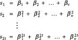
These 2t equations are symmetric functions in β_l, β₂,…, β_v that are known as power-sum symmetric functions.

Next, define σ(x) as

(D.11)

The roots of σ(x), β₁,β₂,…,β_v are the inverses of the error-location numbers. For this reason, σ(x) is called the error-location polynomial.

The coefficients of σ(x) and the error-location numbers are related by

(D.12)

The σ_i are called elementary symmetric functions of the β₁s. The σ_i´s are related to the s_j by

(D.13)

These are called Newton’s identities. These must be solved for the σ(x) of minimum degree.

Step 3 Finding the Error-Location Numbers and Error Correction

The last step in decoding a BCH code is to find the error-location numbers that are the reciprocals of the roots of σ(x). The roots of σ(x) can be found by substituting 1, α, α²,…, α^η-1 into σ(x). If α^l is a root of σ(x), α^n-l is an error-location number and the received digit r_n-l is an erroneous digit.

D.1.2 Iterative Procedure (Berlekamp’s Algorithm)

The iteration number is a superscript, σ^(μ)(x). The first iteration is to find a minimum-degree polynomial σ⁽¹⁾(x) whose coefficients satisfy the first Newton identity.

For the second iteration, check if σ⁽¹⁾(x) satisfies the second Newton identity. If it does, σ⁽²⁾(x) = σ⁽¹⁾(x). If the coefficients of σ⁽¹⁾(x) do not satisfy the second Newton identity, a correction term is added to σ⁽¹⁾(x) to form σ⁽²⁾(x) such that σ⁽²⁾(x) has minimum degree and its coefficients satisfy the first two Newton identities.

This procedure is continued until σ^(2t)(x) is obtained. Then,

To calculate the discrepancy, let

be the minimum-degree polynomial determined at the μth iteration whose coefficients satisfy the first μ Newton identities. To determine σ^(μ+1)(x) we compute the μth discrepancy:

If d_μ = 0, then σ^(μ+1)(x) = σ^(μ)(x). However, if d_μ 0, go back to the iteration number less than μ and determine a polynomial σ^ρ(x) such that the ρth discrepancy d_ρ 0 and ρ – l_ρ has the largest value. Then,

(D.14)

To carry out the iterations of finding σ(x), we begin with Table D.1 and fill out the rows where l_μ is the degree of σ^(μ)(X).

Table D.1 Iterative Algorithm for σ^(μ)(x)

If we have filled Table D.1 through the μth row, the μ + 1 row is calculated as follows:

1. If d_μ = 0, then σ^(μ+1)(x) =σ^(μ)(x) and l_μ+1 = l_μ.

2. If d_μ 0, find another row ρ prior to the μth row such that d_ρ 0 and the number ρ – l_ρ in the last column of the table has the largest value. Then σ^(μ+1)(x) is given by Equation (D.14) and

3. In either case,

If the number of errors in the received polynomial is less than the designed error-correcting capability t of the code, it is not necessary to carry out the 2t steps for finding σ(x). It can be shown that if σ^(μ)(x) and if d_μ and the discrepancies at the next t – l_μ – 1 iterations are 0, the solution is σ^(μ)(x).

While this is interesting and can reduce the average computation time, it leads to variable rate decoding. Since decoding a particular vector may take all 2t steps, most systems will be designed to allow this amount of time for decoding.