
Chapter Eight. MPEG 2 Video Compression
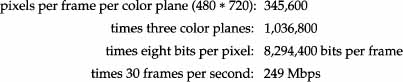
Suppose video is represented by frames of 480 pixels vertical by 720 pixels horizontal (the approximate size of CCIR 601-1). These are arrays of numbers that range from 0 to 255, with the value representing the intensity of the image at that point. This video is to be displayed at 30 frames per second.
There are three color planes (and hence three arrays). The bit rate for this video can thus be calculated as:
8.1 The Need for Video Compression
Most studies have shown that the economics of a DBS system require from four to eight TV channels per transponder. If the information bit rate per transponder is 30 Mbps, the total bit rate (video, audio, and other data) must be 3.75 Mbps to 7.5 Mbps (on average) per audio and/or video service. The audio and data will require approximately 0.2 Mbps per service. Thus, the video must be between 3.55 Mbps and 7.3 Mbps. Comparing this to the uncompressed 249 Mbps, it is clear that the video has to be compressed by 34 to 70 to 1 in order to have an economically viable DBS system. This chapter explains how this is achieved.
8.2 Profiles and Levels
All MPEG standards are generated as generic. This means that they are intended to provide compression for a wide variety of applications. The MPEG 2 Video standard lists a large number of possible applications, including DBS.
The extremely wide range of applications requires a commensurately large range of bit rates, resolutions, and video quality. To cope with this wide range of parameters, MPEG Video uses the concept of Profiles and Levels.
A Profile is a defined subset of the entire bitstream syntax. Within the bounds of a particular profile, there is a wide range of permissible parameters. Levels indicate this range. The Profiles and Levels are orthogonal axes. Section 8 of ISO 13818-2 has a number of tables that define the Profile and Level parameters.
For example, the Maximum Bit Rate table shows that the maximum bit rate for the Main Profile can range from 15 Mbps for the Main Level to 80 Mbps for the High Level. While there are five Profiles and four Levels, only 11 of the combinations have entries in the ISO table. The other nine entries are not defined. The following are the defined Profiles and Levels:
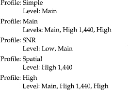
These Profiles and Levels cover an extremely wide range of video parameters; however, all known DBS systems currently use Main Profile at Main Level (written MP@ML). Thus, although High Profile may be used for DBS in the future, except for Chapter 13 where we address future services, the remainder of this book covers MP@ML.
8.3 Digital Video Primer
Digital video is a sequence of frames in which the individual frames are considered to be samples of an analog image on a rectangular sampling grid. The individual samples are called picture elements, or pixels. This is a very good model when the acquisition device is a CCD camera; when film is digitized; or when an analog camera’s output is sampled, held, and then converted to a digital format by an analog-to-digital converter.
8.3.1 Color
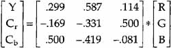
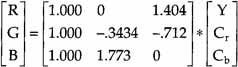
To produce a color image, three color axes are required. Most acquisition and display devices use the additive primaries—red, green, and blue (RGB)—to achieve this. However, the RGB axes are correlated with each other. Thus, virtually all compression algorithms perform a preprocessing step of color coordinate conversion that creates a luminance component (Y) and two chrominance components (Cr and Cb). The Y component displayed by itself is the black-and-white video. At the decoder output, a postprocessing step converts the color space back to RGB for display.
The color coordinate conversion consists of multiplying a three-component vector (RGB) by a 3-by-3 matrix.
At the output of the decoder, a post-processing step converts the [Y, Cr, Cb] vector back to [R, G, B] by the following matrix/vector multiplication.
8.3.2 Interlace
In the 1930s, when TV was being developed, the cathode ray tube (CRT) was the only choice available as a display device. At 30 frames per second,1 the flicker on the CRT was unacceptable. To solve this, the TV developers invented the concept of interlace.
1 The NTSC values are used here. For PAL or SECAM, the frame rate is 25 frames per second and the field rate is 50 fields per second.
Interlaced frames are separated into two fields. Temporally, the rate of the fields is 60 fields per second, twice the frame rate. This refresh rate makes the flicker acceptable (actually, some flicker can be seen at 60 fields per second; at 72 fields per second, it disappears entirely).
Spatially, the horizontal lines from the two fields are interleaved as shown in Figure 8.1. It is frequently claimed that interlace provides a bandwidth compression of 2:1. This is nonsense. While the bandwidth required is half of what would be required if the frames were sent at the field rate, only half the information is sent with each field.
Figure 8.1 Interlace Frame
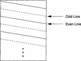
A display that presents the frame lines sequentially is called progressive. At this point in time, technology has developed to where progressive display is economically feasible, and it would significantly improve image quality. However, virtually all of the 2 to 3 billion TV sets in the world use interlace, so any DBS system must be able to accommodate interlacing.
8.3.3 Chroma Subsampling
To achieve the best quality, digital video should be sampled on a grid with equal numbers of samples for each of the three color planes. However, TV engineers discovered that the Human Vision System (HVS) is less sensitive to resolution in the Cr and Cb axes (the color axes) than on the Y, or luminance, axis. It is not surprising that this lesser sensitivity to Cr and Cb was taken advantage of, given the huge amounts of data generated by digital video.
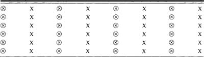
The CCIR 601-1 Standard for recording digital video uses ‘4:2:2’ chroma subsampling. In digital terms, this means that the Cr and Cb chroma planes are decimated horizontally by a factor of two relative to the luma. If the color planes at origination are 480-by-720 pixels, after this decimation the luminance plane is still 480-by-720 pixels, but the Cr and Cb axes are each 480-by-360 pixels. Another way of stating this is that the bits per pixel have been reduced from 24 (8 for each color plane) to 16, a compression of one-third. Table 8.1 shows the relative location of the luminance (X) and chrominance (O) samples for 4:2:2 sampling. The circled X 0 is for both Cr and Cb samples.
Table 8.1 Position of Luminance and Chrominance Samples 4:2:2
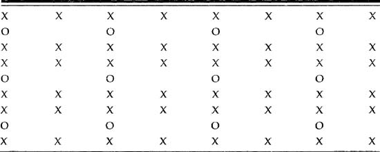
The developers of the MPEG standard took another step. Because the decimation of Cr and Cb in the horizontal direction is asymmetric, they also explored decimation in the vertical direction. This led to the ‘4:2:0’ sampling structure that decimates the Cr and Cb color planes vertically as well as horizontally. Thus, while the Y plane remains at 480-by-720 pixels, the Cr and Cb color planes are 240-by-360 pixels. Table 8.2 shows the position of the luminance and chrominance samples for 4:2:0. The O represents both Cr and Cb samples.
Table 8.2 Position of Luminance and Chrominance Samples 4:2:0
The additional decimation vertically reduces the aggregate bits per pixel to 12. Thus, the 4:2:0 sampling has produced an initial compression of 2:1.
8.4 Structure of MPEG 2 Coded Video
The structure of the coded video data has a nested hierarchy of headers and the following coded data, which can comprise six levels:
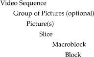
When the decoding of the MPEG 2 Video bitstream is discussed in section 8.6, it will be shown that the problem is to start with a bitstream and parse it down to an 8-by-8 Block, which can then be recreated for display.
The beginning of each of the levels in the hierarchy is indicated by a unique 32-bit (eight-hex character) start code. The first six hex characters are common to all of the codes: 0x000001. A two-hex character suffix, which is unique to the particular level, is then added. In the rest of this chapter only the two-hex character codes are used—the picture_start_code = 0x00. The slice_start_code ranges from 0x01 to OxAF. These sequentially indicate the Slices within a picture. The remainder of the codes in MPEG 2 Video are of the form OxBX, where X ranges from 0 to 8. Three of these, OxBO, OxBl, and OxB6, are reserved. Of the remaining six, three involve the Sequence level—sequence_header_code (OxB3), sequence_ error_code (OxB4), and sequence_ end_code (OxB7). The remaining three are: user_data_start_code (OxB2), extension_start_code (OxB5), and group_start_ code (OxB8).
8.4.1 Video Sequence
The Video Sequence is the highest-level structure in the hierarchy. It begins with a sequence header, sequence_header_code (OxB3), that may then be followed by a Group of Pictures (GOP) header and one or more coded frames. The order of transmission of the frames is the order in which the decoder processes them, but not necessarily the correct order for display.
After the sequence_header_code, the sequence header contains information about the video, which usually won’t change too often. This includes information about the horizontal and vertical sizes (horizon tal_size_value and vertical_size_value) that are unsigned 12-bit integers. Thus, without extensions, a 4,096-by-4096 pixel image size can be specified.
The aspect ratio in Video is the ratio of the number of horizontal pixels to the number of vertical pixels in a frame. The parameter aspect_ratio_ information, which contains 4 bits, provides this information. The value ‘0000’ is forbidden. A square picture (1:1 aspect ratio) has the code ‘0001’. The standard TV aspect ratio (4:3) has the code ‘0010’. The 16:9 ratio code is ‘0011’ and a 2.21:1 ratio code is ‘0100’.
The frame_rate_code is another 4-bit unsigned integer that indicates the frame rate. The code ‘0000’ is forbidden. The values ‘1001’ through ‘1111’ are reserved. Codes ‘0001’ to ‘1000’ indicate 23.976,24,25,29.97,30,50,59.94, and 60 frames per second.
The bit rate is a 30-bit integer. It indicates the bit rate in multiples of 400 bps. The lower 18 bits are indicated by bit_rate_value. The upper 12 bits are in bit_rate_extension, which is contained in sequence_extension.
The next parameter in the sequence_header is a single bit, which is always a ‘1’, called the marker_bit. It is included to prevent start_code emulation.
Next comes the vbv_buffer_size_value. The parameter vbv_buffer_size is an 18-bit integer that defines the size of the buffer in the decoder. The first 10 bits of this value are given by vbv_buffer_size_value. The value of the buffer size is B = 16,384 * vbv_buffer_size bits. The upper 8 bits are in vbv_ buffer_size_extension, which is in sequence_extension.
To facilitate the use of simple decoders in MPEG 1, a set of constrained parameters are defined. For MPEG 2 Video, this doesn’t apply, so the 1-bit flag, constrained_parameters_flag, is always set to ‘0’.
The last parameters of the sequence_header permit the sending of quantization matrices. If an Intra quantizer matrix is to be sent, the 1-bit flag, load_intra_quantizer_matrix, is set to ‘1’. There then follow 64 8-bit values for intra_quantizer_matrix[64]. A similar option is available for non-Intra quantizer matrices.
In a normal Video sequence, the sequence_header is followed by a sequence_extension that has the start_code 0x000001B5. The next item in the sequence_extension is a 4-bit extension_start_code_identifier, which indicates the type of extension. The values ‘0000’, ‘0100’, ‘0110’, and ‘1011’ through ‘1111’ are reserved. Three of the extension_start_code_identifier codes involve the Sequence Extension—Sequence Extension ID (‘0001’), Sequence Display Extension ID (‘0010’), and Sequence Scalable Extension ID (‘0101’).
Four of the extension_start_code_identifier codes involve Picture coding: Picture Display Extension ID (‘0111’), Picture Coding Extension ID (‘1000’), Picture Spatial Scalable Extension ID (‘1000’), and Picture Temporal Scalable Extension ID (‘1000’). The final extension_start_code_identifier code is the Quant Matrix Extension ID (‘0011’). If the extension_start_code_ identifier indicates that the extension is a regular sequence extension, the following are the parameters.
Since DBS uses only MP@ML, the parameter profile_and-level_ indication has the value 0x48. The 1-bit flag, progressive_sequence, is set to ‘1’ if the display mode is progressive. The parameter chroma_format is a 2-bit code that indicates whether the chroma sampling is 4:2:0 (‘01’), 4:2:2 (‘10’), or 4:4:4 (‘11’). The value ‘00’ is reserved.
The horizontal_size_extension and the vertical_size_extension are 2-bit unsigned integers that can be prefixes to horizontal_size_value and vertical_ size_value, increasing the horizontal and vertical sizes up to 14 bits. The most significant part of the bit rate is provided by the 12-bit bit_rate_ extension. Again, a marker_bit that is always ‘1’ is inserted to prevent start_code emulation. The eight most significant bits of the buffer size are provided by vbv_buffer_size_extension.
In some applications where delay is important, no B Pictures are used. This is indicated by the 1-bit flag, low_delay, being set to ‘1’. For non-standard frame rates, the actual frame rate can be calculated from the parameters frame_rate_extension_n (2 bits) and frame_rate_extension_d (5 bits) along with frame_rate_value from the sequence_header. The calculation is frame_rate = frame_rate_value * (frame_rate_extension_n + frame_rate_ extension_d).
The Sequence Display Extension contains information as to which Video format is used (NTSC (‘010’), PAL (‘001’), SECAM (‘011’), and so on) in the parameter video_format. The 1-bit flag colour_description indicates if there is a change in the three 8-bit value parameters—colour_primaries, transfer_ characteristics, and matrix_coefficients. Since these are detailed descriptions of the color, they won’t be discussed further.
The 14-bit unsigned integer display_horizontal_size permits designating the horizontal size of the display. The inevitable marker_bit, always ‘1’, prevents start_code emulation. Finally, the 14-bit unsigned integer, display_vertical_size, permits designating the display’s vertical size.
The Sequence Scalable Extension is not used in DBS, so it is not discussed here.
The Video Sequence is terminated by a sequence_end_code. At various points in the Video Sequence, a coded frame may be preceded by a repeat sequence header, a Group of Pictures header, or both.
8.4.2 Group of Pictures
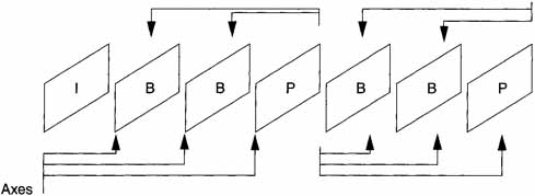
The GOP is a set of pictures, which includes frames that do not require information from any other frames that occur before or after (defined as Intra, or I frames), frames that are unidirectionally predicted from a prior frame (defined as P frames), and frames that are bidirectionally predicted from prior and later frames (defined as B frames). Figure 8.2a shows a typical GOP. The header for a GOP is optional.
Figure 8.2a Structure of Intraframe Coding
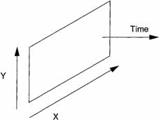
It is natural to ask why different types of frames are needed. Figure 8.2b shows a typical frame (it could be I, P, or B). To achieve the maximum compression, redundancies must be removed from three axes: two spatial and one temporal. The P and B frames are used to achieve temporal compression. Studies have shown that P frames require only 40% as many bits and B frames require only 10% as many bits as those needed for I frames.
Figure 8.2b Remove Redundancies on Three Axes
The structure shown in Figure 8.2a is usually called a hybrid coder. This is because spatial compression is achieved by transform techniques and temporal compression by motion compensation. There is a feature of MPEG compression implied by Figure 8.2a that is difficult to understand for those seeing it for the first time.
Because B frames must be created from prior I or P frames and subsequent I or P frames, the decoder must have both before the B frames can be decoded. Thus, the order of transmission cannot be the IBBPBBP … for both acquisition and display. Rather, the order must be IPBBPBBP.… Note that this puts restrictions on the encoder because it must store the frames that are going to become B frames until the frame that is going to be the following I or P frame is input into the encoder. It also increases the latency—the time from when encoding starts for a frame until display starts for that frame.
When the bitstream includes a Group of Pictures header, the following parameters are included. The group_start_code is 0xB8. A 25-bit binary string indicates the time_code in hours (5 bits), minutes (6 bits), and seconds (6 bits). Since there can be up to 60 pictures per second, there is a 6-bit parameter time_code_pictures, which counts the pictures. The time_code starts with a 1-bit flag, drop_frame_flag, which is ‘1’ only if the frame rate is 29.97 frames per second. A marker_bit, always ‘1’, is located between time_code_minutes and time_code_seconds. The 1-bit flags, closed_gop and broken_link, involve treatment of B frames following the first I frame after the GOP header.
8.4.3 Picture (Frame)
Pictures are the basic unit that is received as input and is output for display. As noted before, coded pictures can be I, B, or P. Pictures also can be either Field Pictures or Frame Pictures. Field Pictures appear in pairs: one top field picture and one bottom field picture that together constitute a frame. When coding interlaced pictures using frame pictures, the two fields are interleaved with each other and coded as a single-frame picture.
The picture_header starts with the picture_start_code 0x00. The next parameter is the temporal_reference, a 10-bit unsigned integer that counts the pictures and wraps around to 0 after reaching 1,023. The next parameter indicates the type of coding, intra_coded (‘001’), predictive_coded (‘010’), or bidirectional_predictive_coded (‘011’). The 16-bit unsigned integer, vbv_delay, provides information on the occupancy of the decoder buffer. There are four parameters—full_pel_forward_vector (1 bit), forward_f_code (3 bits), full_pel_backward_vector (1 bit), and backward_f_code (3 bits)—that are not used in MPEG 2 Video. The 1-bit parameter extra_bit_picture is always set to ‘0’.
Pictures are subdivided into Slices, Macroblocks, and Blocks, each of which has its own header.
Slice
A Macroblock is comprised of 16-by-16 pixels. A Slice is a row or partial row of Macroblocks. Dividing Pictures into Slices is one of the innovations of MPEG compression. If data becomes corrupted in transmission, it may be confined to a single Slice, in which case the decoder can discard just that Slice but not the whole Picture. The Slice header also contains a quantizer scale factor, which permits the decoder to adjust the dequantization.
Figure 8.3 shows the general structure of a Slice. Note that it is not necessary for Slices to cover the entire Picture. Also, Slices may not overlap and the location of the Slices may change from Picture to Picture.
Figure 8.3 General Slice Structure

The first and last Macroblock of a Slice must be on the same horizontal row of Macroblocks. Slices also must appear in the bitstream in the order they appear in the Picture (in normal raster order, that is, left to right and top to bottom). Under certain circumstances a restricted Slice structure must be used. In this case, each Slice is a complete row of Macroblocks and the Slices cover the entire Picture.
The slice_header has the start codes 0x01 through 0xAF. The slice_ vertical_position is the last 8 bits of the slice_start_code. For very large pictures, with more than 2,800 lines, there is a parameter slice_vertical_ position_extension, which gives the Slice location. Because this does not apply to DBS, the calculation for it will not be given.
The parameter priority_breakpoint is a 7-bit unsigned integer that is used only in scalable modes and hence, not in DBS. The scalar quantizer is a 5-bit parameter with values ranging from 1 to 31. It stays the same until another value occurs in a Slice or Macroblock. The 1-bit intra_slice_flag is set to ‘1’ if there are intra-Slice and reserved bits in the bitstream. If any of the Macroblocks in the Slice are non-Intra Macroblocks, the intra_slice is set to ‘0’, otherwise, it is ‘1’.
There are 7 bits of unsigned integer that are reserved, logically enough reserved_bits. The next bit is extra_bit_slice. If it is ‘1’, 8 unsigned integer bits follow. This is a provision for future expansion. If extra_bit_slice is ‘0’, the coding of Macroblocks within the Slice proceeds.
Macroblock
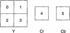
As noted earlier, a luminance Macroblock is a 16-by-16 pixel region. The chrominance part of a Macroblock depends on the chrominance sampling. Since only MP@ML is being considered in this book, the chrominance sampling is 4:2:0 and the Macroblock structure is that shown in Figure 8.4. Note that the Macroblock for 4:2:0 coding is comprised of six blocks. The luminance component has four 8-by-8 blocks and the chrominance components have one 8-by-8 block each.
Figure 8.4. Macroblock Structure for 4:2:0
Macroblocks are the basic unit of coding for motion compensation. Motion vectors are determined for the luminance Macroblock and the motion vectors for chrominance are determined from the luminance motion vectors.
In Frame DCT coding, each Block is composed of lines from both fields (odd and even lines) in the same order they are displayed (i.e., odd, even, odd,…). The Macroblock is divided into four Blocks as always. In Field DCT coding, each Block is composed of lines from only odd or only even lines.
Macroblocks do not have a header. Their encoding proceeds sequentially within a Slice. From Figure 8.3 it is clear that the addresses of Macroblocks are not necessarily sequential. If the address difference is greater than 33, the 11-bit binary string ‘0000 0001 000’, macroblock_escape, indicates that 33 should be added to the value indicated by macroblock_address_increment, a 1- to 11-bit variable length code. The increment value ranges from 1 to 33.
A 5-bit quantizer_scale_code follows next in the Macroblock. The presence of this parameter in each Macroblock is important—it allows quantization to be changed in every Macroblock. This means that an MPEG 2 Video Intra frame is much more efficient than an original JPEG-coded image in which the quantization had to be set once for the picture (JPEG corrected this in later versions). Finally, there is a marker_bit, always ‘1’.
Block
Blocks are 8-by-8 pixels and are the smallest syntactic unit of MPEG Video. Blocks are the basic unit for DCT coding.
8.5 Detailed MPEG 2 Coding of Pictures
As previously noted, MPEG 2 Video compression consists of a spatial compression step and a temporal compression step. These are discussed in the following sections.
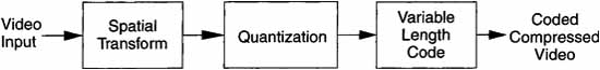
Spatial Compression: Figure 8.5 shows the three major steps in spatial compression. First, the image pixels are transformed by an 8-by-8 block Discrete Cosine Transform (DCT). Next, the transform coefficients are quantized. Finally, the quantized coefficients are encoded with a variable length code (VLC). Note that the transform step and the variable length coding step are one-to-one mappings; therefore, the only losses in the spatial compression are generated in the quantization step.
Figure 8.5 Spatial Compression Steps
8.5.1 I Pictures
Spatial Transform
Before starting a detailed discussion of the DCT, it is important to understand the role of the transform. The input to the transform is an 8-by-8 array of pixels from an image in which the intensity value of each pixel in each color plane ranges from 0 to 255. The output is another array of 8-by-8 numbers. The spatial transform takes the 8-by-8 element image Block and transforms it into the 8-by-8 transform coefficient Block, which can be coded with vastly fewer bits than can the original input Block.
The (0,0) transform coefficient is special. It represents the average value of the 64 input pixels and is called the DC value. As one moves to the right in the horizontal direction, or down in the vertical direction, the transform characterizations are said to be of increasing spatial frequency, where spatial frequency is a measure of the edge content or how close things are together. High spatial frequency corresponds to edges or where things are closer together. As with other similar one-dimensional counterparts, there is an inverse relationship between things being close together and high spatial frequencies. The DCT is effective because it tends to concentrate the energy in the transform coefficients in the upper-left corner of the array, which are the lower spatial frequencies.
The DCT: The N-by-N block DCT is defined as follows:
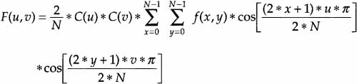
with u, v, x, y equal to 0, 1, … , and 7, where x and y are spatial coordinates in the sample domain, u and v are coordinates in the transform domain, and
![]()
This can be particularized to the 8-by-8 case by setting N = 8.
Final Note about DCT: The optimum transform would be a Karhunen Loeve (KL) transform; however, the KL transform is very computationally intensive and data dependent. It turns out that if the underlying process to be transformed is first-order Markov, the DCT is nearly equivalent to the KL with much less computation required. Video is not quite first-order Markov, but sufficiently close so that, typically, DCT works very well. This is the reason the DCT is used in all major Video compression standards today.
Quantization
The second step of spatial compression is quantization of the transform coefficients, which reduces the number of bits used to represent a DCT coefficient. Because of the multiples used in the DCT, even though the input values are 8 bits, the DCT coefficients could be 11 bits if they were represented exactly. However, this would be extremely wasteful. Quantization is implemented by dividing the transform coefficient by an integer and then rounding to the nearest integer.
The integer divisor of each DCT coefficient is comprised of two parts. The first part is unique for each coefficient in the 8-by-8 DCT matrix. The set of these unique integers is itself a matrix and is called the Quant matrix.
The second part is an integer (quantizer_scale) that is fixed for at least each Macroblock. Thus, if Dct[i][j] is the DCT matrix, then the quantized DCT matrix, Qdct[i][j], is
Qdct[i][j] = 8 * Dct[i][j]/((quantizer_scale) * Q[i][j]).
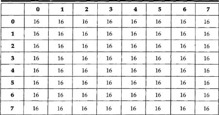
For the nonscalable parts of MPEG 2, which are of primary interest for current DBS, there are two default Quant matrices, one for Intra frames and a second for non-Intra frames. These two default matrices are shown in Tables 8.3 and 8.4.
Table 8.3 Quantization Matrix for Intra Blocks
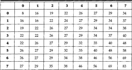
Table 8.4 Quantization Matrix for Non-Intra Blocks
Variable Length Code
Zig Zag Scan: The next step in spatial compression is to map the quantized DCT coefficients into a one-dimensional vector that will be the stub for the Variable Length tables. This mapping is called a zig zag scan. Two zig zag scans are shown in Figures 8.6 and 8.7, one for progressive and the other for interlaced.
Figure 8.6 Zig Zag Scan for Progressive Frames
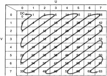
Figure 8.7 Zig Zag Scan for Interlaced Frames
Codebook
After the quantized DCT coefficients have been mapped onto a one-dimensional vector, this vector becomes the stub for a variable length codebook. The purpose of the VLC is to minimize the average number of bits required to code this vector. Those readers who have studied Morse code have already encountered variable length code. The Morse code is based on the frequency of the occurrence of letters in the English language. For example, the letter “e” occurs about 13% of the time, is the most frequent, and thus has the code dot. The VLC for representing the zig zag output is also based on frequency of occurrence.
The VLCs used in MPEG 2 Video are known in Information Theory as Huffman codes. Huffman codes are compact codes, which means that if the underlying statistics are constant, no other code can have a shorter average length.
The Huffman codebook for DCT coefficients is based on the concept of run-length coding. In this technique, the number of consecutive zeroes becomes part of the codebook stub. It is unusual in that the stub includes not only a run length, but also the amplitude of the coefficient that ended the run. As an example, consider Table 8.5, which contains the first few entries from Table B-14 of ISO 13818-2.
Table 8.5 The Shortest Ten of DCT Huffman codes
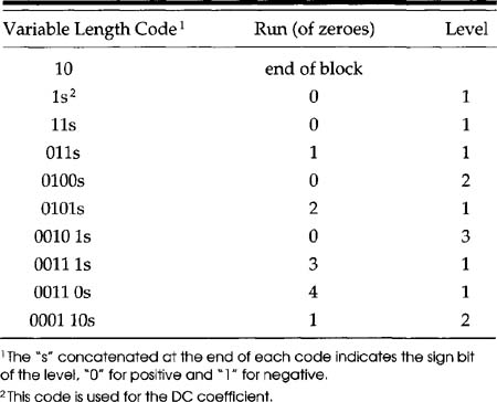
Study of Table 8.5 shows the importance of getting the first few entries of the codebook correct. By just the tenth code, the code is seven bits long, compared with two bits for the shortest code—an increase of 3.5. By the end of Table B.14, the entries are 17 bits long!
8.5.2 P Pictures
P Pictures are predicted from prior I or P frames. There may or may not be intervening B Pictures. The prior I or P frame used to predict a P Picture is called the reference picture. The prediction of a P Picture is comprised of two separate steps: Motion Compensation and Residual Image coding.
Motion Compensation
If the video from a camera pointed at the sky was being encoded, there would be very little change in the pixel values from frame to frame. If a 16-by-16 pixel block were being encoded, its values could be predicted almost exactly from the same area of the reference frame. Thus, we do not have to code the block at all. Instead, we could send a code that tells the decoder to use only the same values from the prior frame. Figure 8.8 depicts motion compensation.
Figure 8.8 Motion Compensation for P Pictures
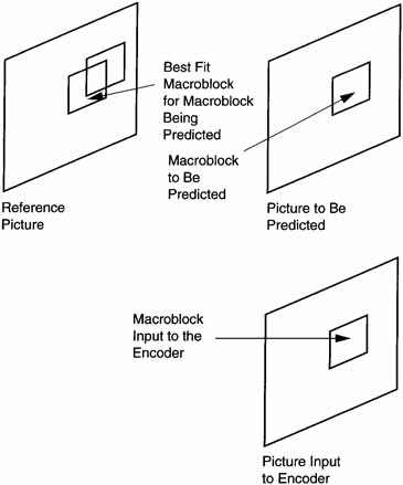
The Macroblock to be predicted has a specific set of coordinates and there is a Macroblock in the input picture that corresponds to this location. Most practical encoders (the encoding process is not defined in ISO 133818-2) use the Macroblock in the input picture at that location to search the reference image in that location for the best fit.
The coordinate offsets in x and y are called motion vectors. Thus, if the motion vectors are coded with a VLC and sent to the decoder, the decoder will locate the coordinate of the current Macroblock being decoded and offset it by the motion vector to select a prediction Macroblock from the reference picture. The 16-by-16 Macroblock of pixels in the reference frame at this offset location becomes the initial prediction for this Macroblock (first step).
It is important that the prediction is where, in the reference frame, the Macroblock came from, rather than where a Macroblock is going. The latter viewpoint would lead to overlaps and cracks in the predicted picture. Three predictions are made: forward prediction, backward prediction, and an average of the forward and backward prediction. The encoder can select which of these is the most efficient.
Residual Image Coding
The quality of the prediction can vary widely. As one example, if a scene was cut between the picture being predicted and the reference picture, there is really no match with the reference frame and the Macroblock has to be coded Intra even though it is in a P Picture. In other cases, the match may be reasonably good overall but poor in a particular location of the Macroblock.
In this case, the reference Macroblock is subtracted from the input Macroblock to form a residual image. This residual image is then coded like the spatial compression shown in Figure 8.5 and discussed previously under I Pictures. In the decoder, the prediction for the Macroblock from motion compensation is first made and then the decoded residual image is added to create the final prediction.
8.5.3 B Pictures
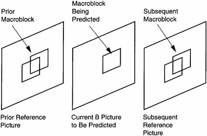
B Pictures are bidirectionally interpolated from reference pictures that precede and succeed the display of the frame being predicted.
Motion Compensation
The use of B Pictures is somewhat controversial, since those seeking maximum compression need them, while those editing these compressed materials have problems because access to frames is required after the frame to be predicted.
Maximum compression is achieved using B Pictures because the residual images of the B Pictures can be heavily quantized without seriously degrading the image quality. This is possible because several pictures of relatively poor quality can be put between “bookend” pictures of good quality without offending the HVS.
Figure 8.9 shows the bidirectional prediction of a B Picture Macroblock.
Figure 8.9 B Picture Motion Prediction
Residual Image Coding
As with P Pictures, a residual image is formed for each Macroblock. These are heavily quantized because a high compression ratio is required for B Pictures.
8.5.4 Coded Block Pattern
The Coded Block Pattern (CBP) is a VLC of 3 to 9 bits that represents a fixed-length, 6-bit code that tells the decoder which Blocks of the Macroblock have nonzero coefficient information. Each Block of a Macroblock is assigned a value; if all the coefficients of a Block are 0, the value is 0. Otherwise, the value is assigned according to this list.

The nonzero values are added to form the CBP and then coded by a VLC. Note that if all Blocks have nonzero values, CBP = 63. If only the luminance Blocks have nonzero coefficients, CBP = 60. It is interesting to note that the value 60 has the shortest VLC (see Table B.9 of ISO 13818-2), which means it is the most frequently occurring value.
8.6 The Video Decoding Process
This section uses the preceding information to describe a complete decoding process.
8.6.1 Recovering the 8-by-8 Pixel Blocks
The decoding process always reverses the encoding process. Thus, the first step is to parse out each of the entities represented by a VLC. The VLC is then inverted to recover the 64-element vector that was coded by the VLC, QFS[n]. An inverse scan then maps QFS[n] into the 8-by-8 array, QF![]() [u]. Inverse quantization creates the array F
[u]. Inverse quantization creates the array F![]() [u]. Finally, the inverse DCT of F
[u]. Finally, the inverse DCT of F![]() [u] forms the 8-by-8 output pixel array, f[x][y].
[u] forms the 8-by-8 output pixel array, f[x][y].
8.6.2 Variable Length Decoding
Variable length decoding is the inverse of the Variable Length Coding process. Since VLC is a 1:1 mapping, the inverse VLC is unique.
DC Component of Intra Blocks
The DC component of the DCT for Intra Blocks is treated differently from all other DCT components. The technique is a form of differential Pulse Code Modulation (PCM). At the beginning of each Slice of an Intra picture, a predictor is set for the DC value for each of the color planes.
In the encoder, a VLC is used to code the parameter dct_dc_size. If dct_dc_size is 0, the DC coefficient for that block is the predictor. If dct_dc_ size is not 0, its value denotes the bit length of a following fixed-length code (up to 11-bits long). It is a differential value that is added to the predictor to create the DC coefficient. The new predictor is this DC value. The reset value of the DC predictor is derived from the parameter intra_dc_precision.
The predictors are defined as dc_dct_pred[cc]. There is a 2-bit parameter called cc (for color component) that takes on the value ‘00’ for luminance blocks, ‘01’ for Cb, and ‘10’ for Cr. Separate codebooks are utilized for luminance dct_dc_size Blocks and chrominance dct_dc_size Blocks.
Other DCT Coefficients
The non-Intra coefficients are decoded from other VLC codebooks. The following are three possibilities.
1. End of block—In this case, there are no more nonzero coefficients in the block and all the remaining coefficients are set to 0.
2. A normal coefficient—This is a combined value of run length and level followed by a single bit designating the sign of the level.
3. An escape code—In this case, special provisions are employed to code the run and level.
8.6.3 Inverse Scan
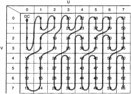
The decoded VLC codes represent a one-dimensional version of the quantized DCT coefficients. In order to inverse quantize these values and then invert the DCT, the one-dimensional vector must be mapped into a two-dimensional matrix. The process of doing this mapping is called the inverse scan.
Table 8.6 shows this mapping for alternate_scan = 0. Note that each entry in the table indicates the position in the two-dimensional array where the one-dimensional index is located. If one examines Figure 8.6, it can be seen that it is identical to Table 8.6; however, in one case the conversion is being made from two dimensions to one dimension, while in the other the reverse is true.
Table 8.6 Inverse Scan for alternate_scan = 0
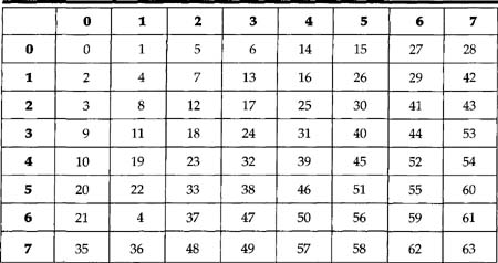
Similarly, the inverse for alternate_scan = 1 is the same as Figure 8.7. When quantization matrices are downloaded, they are encoded in the bit-stream in this same scan order.
8.6.4 Inverse Quantization
The two-dimensional array of coefficients QF![]() [u] is Inverse Quantized to produce the reconstructed DCT coefficients. The process is essentially multiplication by the quantizer step size. This step size is modified by two different entities: (1) a weighting matrix (W
[u] is Inverse Quantized to produce the reconstructed DCT coefficients. The process is essentially multiplication by the quantizer step size. This step size is modified by two different entities: (1) a weighting matrix (W![]()
![]() [u]) modifies the step size within a Block, usually affecting each spatial frequency position differently, and (2) a scalar value (quant_scale) so that the step size can be modified at the cost of a few bits. The output of the first step of the Inverse Quantization is F’[u]
[u]) modifies the step size within a Block, usually affecting each spatial frequency position differently, and (2) a scalar value (quant_scale) so that the step size can be modified at the cost of a few bits. The output of the first step of the Inverse Quantization is F’[u]![]() .
.
Intra-DC Coefficients
The DC coefficients for Intra-coded Blocks are coded differently from all other coefficients. Thus, for Intra Blocks, F’[0][0] = intra_dc_mult * QF[0][0].
Other Coefficients
All other Intra coefficients and all non-Intra coefficients are coded as described in the following sections.
Weighting Matrices
For MP@ML, two matrices are used, one for Intra and one for non-Intra. W![]() [i>][u] represents the weighting matrices (see Tables 8.3 and 8.4). The parameter w is determined from the parameter cc. For 4:2:0, cc = 0 for Intra Blocks and cc = 1 for non-Intra Blocks. For 4:2:2 and 4:4:4 for luminance,
[i>][u] represents the weighting matrices (see Tables 8.3 and 8.4). The parameter w is determined from the parameter cc. For 4:2:0, cc = 0 for Intra Blocks and cc = 1 for non-Intra Blocks. For 4:2:2 and 4:4:4 for luminance, ![]() = 0 for Intra Blocks if cc = 0, for luminance and non-Intra Blocks, if cc = 0,
= 0 for Intra Blocks if cc = 0, for luminance and non-Intra Blocks, if cc = 0, ![]() = 1; for chrominance and Intra Blocks, if cc = 1,
= 1; for chrominance and Intra Blocks, if cc = 1, ![]() = 2, and for chrominance and non-Intra Blocks, if cc = 1,
= 2, and for chrominance and non-Intra Blocks, if cc = 1, ![]() = 3.
= 3.
Quantizer Scale Factor
The parameter quant_scale is needed in the inverse quantization process. The 1-bit flag, q_scale_type, which is coded in the picture extension, and the parameter quantizer_scale_code (contained in the Slice header) determine quant_scale. If q_scale_type = 0, then quant_scale equals two times the quantizer_scale_code. If q_scale_type = 1, quant_scale equals quantizer_scale_code for quantizer_scale_code from 1 to 8. For quantizer_scale_code from 9 to 16, quant_scale = 2 * quantizer_scale_code – 8. For quantizer_ scale_code from 17 to 24, quant_scale = 4 * quantizer_scale_code – 40. For quantizer_scale_code from 25 to 31, quant_scale = 8 * quantizer_scale_ code -136.
Reconstruction of the DCT Coefficient Matrix
The first step in this reconstruction is to form F’![]() [u], where
[u], where
F’![]() [u] = (2 * QF
[u] = (2 * QF![]() [u] + k) * (k * W
[u] + k) * (k * W![]()
![]() [u]) * (quantizer_scale))/32,
[u]) * (quantizer_scale))/32,
where k = 0 for Intra Blocks and k = sine[QF ![]() [u]] for non-Intra Blocks.
[u]] for non-Intra Blocks.
Saturation
For the inverse DCT to work properly, the input range must be restricted to the range 2,047 ≥ F’![]() [u] ≥ -2,048. Thus,
[u] ≥ -2,048. Thus,
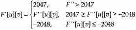
This function, which electronics engineers would call a limiter, is called saturation in MPEG 2.
Mismatch Control
The sum of the coefficients to the Inverse DCT must be odd. Thus, all the coefficients of F’![]() [u] are summed. If the sum is odd, all the coefficients of F
[u] are summed. If the sum is odd, all the coefficients of F![]() [u] are the same as F’
[u] are the same as F’![]() [u]. If the sum is even, F[7][7] is modified. If F’[7][7] is odd, F[7][7] = F[7][7] – 1; if F[7][7] is even, F[7][7] = F’[7][7] + 1. This ensures that the sum of the coefficients input to the inverse DCT is odd.
[u]. If the sum is even, F[7][7] is modified. If F’[7][7] is odd, F[7][7] = F[7][7] – 1; if F[7][7] is even, F[7][7] = F’[7][7] + 1. This ensures that the sum of the coefficients input to the inverse DCT is odd.
8.6.5 Inverse DCT
Finally, the inverse DCT recreates the spatial values for each Block using the following equation:
![]()
where N is set to 8 for the 8-by-8 blocks.
8.6.6 Motion Compensation
Figure 8.10 is an overview of the motion compensation output. The output of the Inverse DCT, f[y][x], is added to the motion prediction output p[y][x]. The sum is then limited to the range 0 to 255 by the Saturation step. The output of the Saturation step is the decoded pixels for display.
Figure 8.10 Overview of Motion Compensation Output
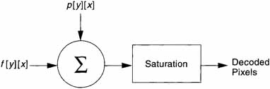
Several things should be noted about Figure 8.10. First, even though the predictions are for Macroblocks, p[y][x] is the appropriate Block of the predicted Macroblock. Second, for the chrominance axes, the decoded pixels out are still 8-by-8 pixels. The decoder must interpolate them to 16-by-16 pixels prior to display. Finally, it should be noted that the output of the Inverse DCT, f[y][x], is from the result of the coding of the residual image; this is why it is added to the prediction.
Combinations of Predictions
The prediction Block, p [y] [x] in Figure 8.10, can be generated from as many as four different types, which are discussed in the following sections.
The transform data /[y][x] is either field organized or frame organized depending on dct_type. If it specifies frame prediction, then for simple frame prediction the only function the decoder has to perform is to average the forward and backward predictions in B Pictures.
If pel_pred_forward[y][x] is the forward prediction and pel_pred_ backward[y][x] is the corresponding backward prediction, then the final prediction is:
pel_pred[y][x] = (pel_pred_forward[y][x] + pel_pred_backward[y][x])/2
For MP@ML, all the predictors are 8-by-8 pixels.
Simple Field Predictions
In the case of simple field predictions, the only processing required is to average the forward and backward predictions as for the simple frame predictions just described.
16-by-8 Motion Compensation
In this prediction mode, separate predictions are formed for the upper 16-by-8 region of the Macroblock and the lower 16-by-8 region of the Macro-block. The predictions for the chrominance components are 8 samples by 4 lines for MP@ML.
Dual Prime
In Dual Prime mode, two predictions are formed for each field in a manner similar to that for backward and forward prediction of B Pictures. If pel_ pred_same_parity is the prediction sample from the same parity field, and pel_pred_opposite_parity is the corresponding sample from the opposite parity, then the final prediction sample is formed as:
pel_pred[y][x] = (pel_pred_same_parity[y][x] + pel_pred_opposite_parity[y][x])/2
In the case of Dual Prime prediction in a frame picture, the predictions for the chrominance components of each field for MP@ML are 8 samples by 4 lines. In the case of Dual Prime prediction in a field picture, the predictions for chrominance components are 8 samples by 8 lines for MP@ML.
8.6.7 Skipped Macroblocks
In Skipped Macroblocks (where macroblock_address_increment is greater than 1), the decoder has neither DCT coefficients nor motion vector information. The decoder has to form a prediction for these Macroblocks that is used as final decoded sample values. The handling of Skipped Macroblocks is different for P Pictures and B Pictures and for field pictures and frame pictures. Macroblocks for I Pictures cannot be skipped.
P Field Pictures
The prediction is made as if field_motion_type is ‘Field based’ and the prediction is made from the field of the same polarity as the field being predicted. Motion vector predictors and motion vectors are set to 0.
P Frame Pictures
The prediction is made as if frame_motion_type is ‘Frame based.’ Motion vector predictors and motion vectors are set to 0.
B Field Pictures
The prediction is made as if field_motion_type is ‘Field based’ and the prediction is made from the field of the same polarity as the field being predicted. The direction of the prediction (forward/backward/bidirectional) is the same as the previous Macroblock. The motion vector predictors are unaffected. The motion vectors are taken from the appropriate motion vector predictors, dividing both the horizontal and vertical components by two scales of the chrominance motion vectors.
B Frame Pictures
The prediction is made as if frame_motion_type is ‘Frame based.’ The direction of the prediction (forward/backward/bidirectional) is the same as the previous Macroblock. The motion vector predictors are unaffected. The motion vectors are taken from the appropriate motion vector predictors, dividing both the horizontal and vertical components by two scales of the chrominance motion vectors.
8.7 Prediction Modes
![]()
There are two major prediction modes: field prediction and frame prediction. (For more detailed information, see Sections 7.1 to 7.5 of ISO 13818-2.)
In field prediction, predictions are made independently for each field by using data from one or more previously decoded fields. Frame prediction forms a prediction for the frame from one or more previously decoded frames. The fields and frames from which predictions are made may themselves have been decoded as either field or frame pictures.
Within a field picture, all predictions are field predictions. However, in a frame picture either field or frame predictions may be used (selected on a Macroblock-by-Macroblock basis).
8.7.1 Special Prediction Modes
In addition to the two major classifications, there are two special prediction modes: 16-by-8 and Dual Prime. Because Dual Prime is used only when there are no B Pictures, it will not be discussed further here.
In 16-by-8 motion compensation, two motion vectors are used for each Macroblock. The first motion vector is used for the upper 16-by-8 region, the second for the lower 16-by-8 region. In the case of bidirectionally interpolated Macroblocks, a total of four motion vectors are required because there will be two for the forward prediction and two for the backward prediction. A16-by-8 prediction is used only with field pictures.
8.7.2 Field and Frame Prediction
The prediction for P and B frames is somewhat different for fields and frames.
Field Prediction
In P Pictures, prediction is made from the two most recently decoded reference fields. In the simplest case, the two reference fields are used to reconstruct the frame, regardless of any intervening B frames.
The reference fields themselves may have been reconstructed by decoding two field pictures or a single frame picture. When predicting a field picture, the field being predicted may be either the top field or the bottom field.
Predicting the second field picture of coded frame uses the two most recently decoded reference fields and the most recent reference field is obtained from decoding the first field picture of the coded frame. When the field to be predicted is the bottom frame, this is the top field; when the field to be predicted is the top field, the bottom field of that frame is used. Once again, intervening B fields are ignored.
Field prediction in B Pictures is made from the two fields of the two most recently reconstructed reference frames, one before and one after the frame being predicted. The reference frames themselves may have been reconstructed from two field pictures or a single frame picture.
Frame Prediction
In P Pictures, prediction is made from the most recently reconstructed reference frame. Similarly, frame prediction in B Pictures is made from the two most recently reconstructed reference frames, one before and one after the frame being predicted.
8.7.3 Motion Vectors
Motion vectors are coded differentially with respect to previously decoded motion vectors. To decode the motion vectors, the decoder must maintain four motion vector predictors (each with a horizontal and vertical component) denoted PMV [r] [s] [t]. For each prediction, a motion vector’ vector [r] [s] [t] is derived first. This is then scaled according to the sampling structure to give another motion vector, vector[r][s][t], for each color component.
The [r][s][t] Triplet
The parameter r determines whether the first motion vector in a Macroblock is indicated with a ‘0’, the second, with a ‘1’. The parameter s indicates whether the motion vector is forward, with a ‘0’, or backward, with a ‘1’. The parameter t indicates whether the motion vector represents a horizontal component, with a ‘0’, or a vertical component, with a ‘1’.
Two types of information are decoded from the bitstream in order to make the prediction: (1) information on the delta to be added to the prediction and (2) which motion vector predictor to use.
Updating Motion Vector Predictors
Once the motion vectors for a Macroblock have been determined, it is necessary to update the motion vector predictors. This is necessary because these predictors may be used on a subsequent Macroblock.
If the frame_motion_type is:
Frame-based and the macroblock_intra is ‘1’, then PMV[1][0][1] = PMV[0][0][1] and PMV[1][0][0] = PMV[0][0][0].
Frame-based and the macroblock_intra is ‘0’, and macroblock_ motion_forward and macroblock_motion_backward are both ‘1’, then PMV[1][0][1] = PMV[0][0][1], PMV[1][0][0] = PMV[0][0][0], PMV[1][1][1] = PMV[0][1][1], and PMV[1][1][0] = PMV[0][1][0].
Frame-based and the macroblock_intra is ‘0’, the macroblock_ motion_forward = ‘1’, and the macroblock_motion_backward = ‘0’, then PMV[1][0][1] = PMV[0][0][1] and PMV[1][0][0] = PMV[0][0][0].
Frame-based and the macroblock_intra is ‘0’, the macroblock_ motion_forward = ‘0’, and the macroblock_motion_backward = ‘1’, then PMV[1][1][1] = PMV[0][1][1] and PMV[1][1][0] = PMV[0][1][0].
Frame-based and the macroblock_intra is ‘0’, the macroblock_ motion_forward = ‘0’, and macroblock_motion_backward = ‘0’, then PMV[r][s][t] = 0 for all r,s,t.
Field-based only, there are no predictors to update.
Dual Prime and macroblock_intra is ‘0’, the macroblock_ motion__ forward = ‘1’, and the macroblock_motion_backward = ‘0’, then PMV[1][0][1] = PMV[0][0][1] and PMV[1][0][0] = PMV[0][0][0].
If the field_motion_type is:
Field-based and the macroblock_intra is ‘1’, then PMV[1][0][1] = PMV[0][0][1] and PMV[1][0][0] = PMV[0][0][0].
Field-based and the macroblock_intra is ‘0’, and macroblock_motion_forward and macroblock_motion_backward are both ‘1’, then PMV[1][0][1] = PMV[0][0][1], PMV[1][0][0] = PMV[0][0][0], PMV[1][1][1] = PMV[0][1][1], and PMV[1][1][0] = PMV[0][1][0].
Field-based and the macroblock_intra is ‘0’, the macroblock_ motion_forward = ‘1’, and the macroblock_motion_backward = ‘0’, then PMV[1][0][1] = PMV[0][0][1] and PMV[1][0][0] = PMV[0][0][0]. Field-based and the macroblock_intra is ‘0’, the macroblock_ motion_forward = ‘0’, and the macroblock_motion_backward = ‘1’, thenPMV[l][l][l] = PMV[0][1][1] and PMV[1][1][0] = PMV[0][1][0]. Field-based and the macroblock_intra is ‘0’, the macroblock_ motion_forward = ‘0’, and macroblock_motion_backward = ‘0’.
Field-based and the macroblock_intra is ‘0’, the macroblock_ motion_forward = ‘0’, and macroblock_motion_backward = ‘0’, then PMV[r][s][t] = O for all r,s,t.
For a 16-by-8 MC, there are no predictors to update.
Dual Prime and macroblock_intra is ‘0’, the macroblock_ motion_ forward = ‘1’, and the macroblock_motion_backward = ‘0’, then PMV[1][0][1] = PMV[0][0][1] and PMV[1][0][0] = PMV[0][0][0].
Resetting Motion Vector Predictors
All motion vector predictors are reset to 0 in the following situations:
• At the start of each slice
• Whenever an Intra Macroblock is decoded that has no concealment motion vectors
• In a P Picture when a non-Intra Macroblock is decoded in which macroblock_motion_forward is 0
• In a P Picture when a Macroblock is skipped
Motion Vectors for Chrominance Components
For MP@ML, both the horizontal and vertical components of the motion vector are scaled by dividing by two:
vector[r][s][0] = vector’[r][s][0]/2
vector[r][s][1] = vector’[r][s][1]/2
Forming Predictions
Predictions are formed by reading prediction samples from the reference fields or frames. A particular sample is predicted by reading the corresponding sample in the reference field or frame offset by the motion vector.
A positive value of the horizontal component of a motion vector indicates that the prediction is made from samples in the reference field or frame that lie to the right of the samples being predicted. A positive value of the vertical component of a motion vector indicates that the prediction is made from samples in the reference field or frame that lie below the samples being predicted.
All motion vectors are specified to an accuracy of one-half sample. The one-half samples are calculated by simple linear interpolation from the actual samples.
In the case of field-based predictions, it is necessary to determine which of the two available fields to use to form the prediction. If motion_vertical_ field_select is 0, the prediction is taken from the top reference field; if it is ‘1’, from the bottom reference field.