

Six Pack. © hansenphoto.com.
Chapter 9 Overview
Chapter 7 discussed neutral balance in the workflow, and this chapter examines why we need to balance for the light’s spectral bias, where in the process we can apply balancing, and how balancing is accomplished. These corrections can be made within the capture workflow, using post-capture software applications, or via output control.
Light Balancing
Photography, whether with conventional film or digital imagining, is about capturing light. The term photography is derived from the Greek words for light and writing, thus reflecting the importance of understanding light to make good images. As explained in Chapter 7, a major problem in balancing a picture so that the colors are captured correctly is the way our perceptual system works. The human perceptual system holds constant as much of the learned world as possible. This constancy has a great effect on our perception of color, as well as our ability to neutralize light. To understand how to better balance images, it is helpful to examine how light functions. Most important is the spectral makeup of light.
Spectral Composition and Balancing
The spectral composition can be defined as the spectral energy distribution (SED). This is a determination of how much of the power of the energy comes from what part of the electromagnetic spectrum. The amount of energy at any wavelength of the spectrum is measured as its relative energy output. When this value is graphed compared to the wavelength a spectral distribution curve results. This curve reveals the color bias of the light.
Spectral energy distribution (SED) This is a measure of how the energy of a particular light is distributed. When graphed as a spectral distribution curve, the height of the graph represents the amount of energy at any point in the spectrum.
The most commonly used light for photography is the sun. When we look at midday sunlight, often referred to as skylight, we can see how the energy is distributed over the visual spectrum. While the light’s energy is greatest at the blue end of the spectrum, relatively high values can be found in all areas of the spectrum except the violet portion. If the light is purely neutral, the curve would be horizontal with even values at all portions of the spectrum; however, because relatively strong energies exist across the spectrum we will see the light as neutral or white light.
Because of the digital sensor’s weakness at the short wavelengths (violet), the higher blue spectral energies in the light have less effect and a natural balancing effect. However, to totally balance the light a small adjustment must be made to the higher end of the spectral energies (red). As the sun moves across the sky, the atmosphere differentially bends the light and changes its color bias from red at dawn and dusk to the more neutral midday color of light. Neutral balancing can remove the color bias from images made at any time of day, but it may be desirable to use a preset light balance to allow the warmth of the sun to be seen in an image at sunrise or sunset.

Figure 9-1 SED of sunlight.
While midday light is not noticeably biased to the blue end of the spectrum, northern light or clear sky open shade is noticeably blue. This is clearly demonstrated with an SED curve. The SED curve for northern light shows that the shorter wavelengths comprise the majority of the strength of the light, with a smaller effect from the higher end of the visible spectrum. In this type of light, the response to blue must be reduced in comparison to the red end of the spectrum. Northern light can be balanced with over-the-lens warming filters, which make it appear as though the warmer end of the spectrum is strengthened; actually, it remains the same but is more effective compared to other areas of the SED. Filtering is not as accurate as electronic balancing, however.

Figure 9-2 SED for northern skylight.
Another type of light commonly used for digital photography is the electronic flash (strobe). While conventional photography uses the same film balance for both daylight and electronic flash, with digital imaging much finer adjustment of the color balance can be accomplished. The SED curve shows that this type of light is similar to daylight but with a slight increase in energy in the blue–green area of the spectrum. Electronic balancing depresses these blue–green energies. While not shown in the spectral distribution curve, an electronic flash puts out high levels of ultraviolet (UV) energy. Many flash heads are coated with a UV filter that is effective for film capture, but because of the inability of camera sensors to effectively capture UV this is not required for digital capture.
Ultraviolet energy (UV) These are wavelengths shorter than visible violet light but longer than x-rays.
Studio lighting may require continuous light sources. The most common continuous light sources are quartz halogen lights. These use a tungsten filament that heats up to generate the light. The SED curve for these incandescent lights is the reverse of that for northern light. The color light from such hot lights is strongly biased toward the red end of the spectrum. Damping the energies at the red end of the spectrum and visually elevating the blue end correct for the redness of the light.
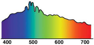
Figure 9-3 SED for the light from an electronic flash.
While not recommended for photographic purposes, occasionally it may be necessary to photograph under fluorescent light. Fluorescent lights generate light by passing electricity through a mercury vapor to produce a large amount of ultraviolet energy. The UV light interacts with phosphors on the inside of the tube which generate the majority of the light. When looking at the SED curve for fluorescent light, we can see that the line spikes from the energized mercury vapor and the light of the phosphors produces a continuous curve. Fluorescent light has a noticeable blue–green cast that must be reduced for neutral balancing.
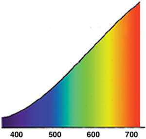
Figure 9-4 SED for tungsten light.
Another type of light used for photographic applications is the metal halide lamp. Most commonly referred to as HMI (Hg [mercury], medium arc, iodine) lamps and also known as metallic halide lamps, these lights are discharge lamps made by adding metal oxides to a small mercury lamp. The addition of the color from the metal oxides’ light discharge that is seen in the closely spaced lines, the SED curve shows a rather even pattern that is biased toward the red within the strong mercury spectrum. The closeness of the lines in the SED created by the metal oxides shows a light source that acts as a continuous source.

Figure 9-5 SED for fluorescent light.

Figure 9-6 SED for light from HMI lighting.
Post-capture operations used to balance neutrality and tonalities in images can be applied to any image format or bit depth; however, there are advantages to using the largest bit depth in the RAW file format if available. If post-capture correction is performed before interpolation at its maximum bit depth, the final image will have fewer artifacts caused by the adjustments. Neutral balancing applies a global correction to the capture of a digital image; however, adjustments to the image may be required to maximize the captured image.
As we begin this discussion of post-capture correction, an important warning must be made: Whenever a digital file is modified in any way, data are lost. For this reason, the originally captured, uncompressed file with the highest bit depth must be saved. Because there is no difference in quality between the original and copies of that original, it is the copies that should be manipulated or altered. The RAW file option is the best choice for archiving the original file.
A key to understanding how images are balanced is the histogram for the image. The histogram is a graph of the number of pixels at each of the digital numbers represented in the image. On the horizontal axis are the digital numbers. In a 24-bit color image (8 bits per channel), the left end of the histogram represents the digital number 0, and the right end represents a value of 255. The vertical axis of the histogram represents the relative number of pixels at a given digital number. While the histogram could use a numerical scale to give an exact count of the pixels at any given digital number, this would result in an unwieldy graph for most uses; therefore, the histogram only gives a proportional representation of these numbers to keep the graph in a reasonable form.
Color images have three histograms, one each for the primary colors of light: red, green, and blue (RGB). An overall histogram is a composite of the individual color histograms; however, when viewing a histogram for a RAW file, all three graphs are shown. In the three-graph version, each channel is displayed on the same graph. Neutral is created where all three colors overlap, and the secondary colors (cyan, magenta, and yellow) are produced where two of the primary colors overlap. Even when the image is interpolated, the three channels can be separated based on the portion of each color represented in each pixel.

Texas Trees. © Kathryn Watts-Martinez.
As an example, if we look at the histogram for a grayscale gradient, we can see a continuous form with no gaps. Now, if we make an adjustment, such as changing the contrast, we notice that the black and white levels stay at the extremes but now there are lines in the histogram. These white lines, known as combing, show where there are no data.
By accepting a certain loss of data, we can process an image to correct a deficiency acquired during the capture process. The two major ways in which image files can be changed are point processes and transforms. A point process is an adjustment that performs the same arithmetic change to every pixel selected for change. Transforms are complicated changes in the image structure such as rotating or warping. Most adjustments are point processes, and filters are transforms. When using image software, point processes, including most adjustments, can be used with 16-bit channels. Most transforms, because of the higher levels of calculations required, are available with only 8-bit-per-channel images.
Point processes Point processes are the simplest computer adjustments; they perform the same operation on every pixel in the image or selected area.
Transforms These are complicated mathematical modifications of the image structure. The computer uses higher-level algorithms to change the image, often one point at a time. Applications such as rotating or warping and most software filters are transforms.

Figure 9-7 The histogram on the left shows the output before adjustment; the histogram on the right shows “combing” after adjustment.
As an example of a point process, if we wanted to brighten an image by 20% we could add a 52 numerical value shift to all pixels. Pure black (0:0:0) would still be dark but brighter in tone (52:52:52). At the same time, a middle gray tone (127:127:127) would become lighter (179:179:179). At the high end of the scale, the values would become compressed. The spikes in the histogram of this shifted tonal scale show the 20% compression. While we get spikes when we shift the output values to brighten the image, combing results if we stretch the levels to move a lighter tone to become black and at the same time maintain the white value. For a 20% value stretch, suppose we move the point with a value of 52 to a value of 0, or the black point. This makes a change for 203 tones in our scale to become an output of 0–255. Here, we can see the 52 steps of stretch in the 52 white lines in the histogram.
These two point process examples were on a grayscale, but the same operations can be performed on individual color channels to shift the color balance. We can add small amounts of color to each of the red, green, and blue channels and in this way correct the color bias in a digital image. The image shown here has a blue bias because the image was shot late at night. A sample of a location on a known neutral wall shows values of 181 for red, 182 for green, and 208 for blue, indicating a blue bias of 26. If the effect of the blue channel can be reduce by 26, then the image will be corrected for the neutral tone. To apply this correction blue can be reduced or red and green can be increased. As an overall point process, these global changes are applied to each pixel equally.
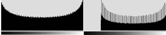
Figure 9-8 The difference in the histograms shows the effect of shifting the black point.

Figure 9-9 The white lines show the stretching to move endpoints of the grayscale.

Figure 9-10 The image on the left shows the blue cast from making an exposure after sunset. The right image shows the image after correcting the image in its three channels.
The simplest adjustment tool is levels, which are linear processes allowing shifts in or stretching of the image’s tonal information in individual channels or as an overall adjustment. These simple adjustments also include brightness, hue/saturation, and color balance. When using a RAW file, this operation can be performed before the image is interpolated and exported for use in other portions of the digital workflow. This is often done to allow shadow detail to be opened up.
Levels Levels are used to modify the distribution of tones in an image in relation to output by changing the white point, black point, and gamma (slope of the curve).
More complex and more useful are curves, which use a graphical approach to analyze an image; that is, changing the shape of the curve adjusts the color. While levels are useful, curves give us the ability to handle specific parts of the tonal range or color channel. This is particularly important in color balancing for color management.
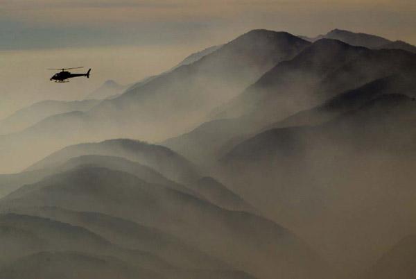
Fire6.AMR. © by Anacleto Rapping—Los Angeles Times.
Curves Curves are graphs in imaging software that show how inputs are related to outputs. In most software packages, the curves can be changed to alter the look of the image.
Curves and Color Balance
Curves are graphic representations of the input tones versus the output tones. The curve is a graph in its default mode that shows a straight line representing the value of input and the value? it will be outputted. A straight line at a 45° angle indicates that any digital number in the image will have a similar number as the output. As the digital number rises, so does the output value. As with a silver halide curve, we describe the top as white in digital or transparency film or as maximum density with negative films, the low point as black for digital and transparency films and the lowest exposure for negative film, and the slope as gamma. If the curve is changed, then the digital output values change. If the bottom scale is reversed by clicking the arrows on the lower scale, the image output becomes negative.

Figure 9-11 Curves dialog box.
There are three tools for using the curve: (1) change the shape of the curve by selecting a point on the curve and moving it, (2) draw the desired curve, or (3) select points in the image and set these selected points into the curve as the white, midtone, and black points. When the curve shape changes it alters the output for the image. For the default curve, with white output at the top right, if the white point is moved horizontally to the left, then the digital value required to output white will be lower. At the same time, the slope of the curve will become steeper, thus increasing the contrast of the image, as there will now be less difference between white and black in the captured image. When the black point is moved horizontally to the right, the black level is actually captured at a tone lighter than black. In the default curve setup, horizontal moves affect the captured values required to create black and white.
In this curve moving the black point upward will make the output for the lowest exposure lighter than true black. Moving the white point down will add grayness to the captured white. At the same time, either of these movements of the curve’s ends lessens the slope and softens the contrast of the image.
By selecting a point on the curve other than at the ends, the curve is bent as the selected point is moved. Selecting multiple points allows for changes in various areas of the curve. If the curve is rounded toward horizontal, the output tones are compressed in relation to the captured values. Rounding the curve toward vertical increases output separations between captured values. While these changes can be accomplished by deforming the existing curve, it can also be drawn and then smoothed out.
The selection tool is used to select points in the image and set the input/output levels on the curve for the selected locations. If a point is selected as black, then that captured level will be set as black output. The same is true for the white and midtone selections. The white and black selections set the end points of the curve, and the mid-tone selector changes the shape of the curve. The shape change bows the curve, increasing or decreasing the slope and the contrast of the image above and below the selection point.
This operation can be performed for red, green, blue (RGB); cyan, magenta, yellow, and black (CMYK); or specific color channels. When working with either RGB or CMYK alone, the color bias is not changed, but using separate color channels allows for color correction. To do this, the curve dialog selector is changed to one of the color channels, and the same actions are taken for each of the channels.
The image shown here was taken on location without standard lighting equipment; thus, after processing the film had a red bias. To correct the image, the curves were changed by selecting the black, white, and mid-tone points for each of the three color channels. The dots on the first image show the three selected points that were used as the black, white, and neutral places in the image and put into the each of the three curves. As selections were made for each point in each channel the curve changed. The end result, after combining the three curves, was an RGB corrected image. The curves indicate the changes in each channel.

Lunaboard. © J. Seeley.

Figure 9-12, Figure 9-13, and Figure 9-14 The first figure shows the image with the curve having black input at the right and black output to the top. The second figure shows an increase in contrast gained by moving the black point (top) and the white point (bottom) toward the center of the graph; this has simply changed the minimum input that will be output as white and the maximum digital number that will be represented as black. This increases the contrast but causes both highlight and shadow details to be lost. The third picture reflects an increase in the contrast for the middle of the curve and a decrease in the contrast for both highlight and shadow details. This has maintained details while changing the contrast for the image.

Many feel that the best color correction can be achieved by using the subtractive CMYK colors instead of correcting for RGB. In order to work in CMYK, the file must be converted from RGB (as captured) to CMYK, which requires another color interpolation. There are two reasons for doing so. First, only CMYK gives a true black–white value scale; in RGB, the curves generate a composite black. The second reason has to do with ultimate use of the image. Most images are printed, and the CMYK family of inks and dyes are used to print images. Some professionals believe using curves in these four channels and adjusting these curves provides better agreement between the image file and the printed output.

Footprints, Death Valley. © 2004 Terry Abrams.

Figure 9-15 The image on the left shows the original image and the points used to adjust the curves to achieve the final image.

Figure 9-16 Three curves used to adjust the image in Figure 9–13. The lower point on each curve shows the adjusted black level, the top point shows the white placement, and the midpoint shapes the curve to adjust for neutrality.
- The spectral energy distribution (SED) shows the amount of light energy at any given wavelength and reveals color bias.
- The SED is the basis for capture-based color balancing.
- Corrections are possible after the image has been made.
- When a digital file is modified, data are lost; therefore, always work on a duplicate file and archive the original capture, preferably as a RAW file.
- Global adjustments are normally point processes that can process 16-bit-per-channel pixels; transforms involve higher-level mathematical functions and can be applied to only 8-bit-per-channel pixels.
- Levels can shift or stretch the tonal range or output range for the total image or individual color channels.
- Curves can adjust the contrast and color balance for the total image or individual channels.
- Some professionals believe that the use of CMYK rather than RGB is beneficial if the final product will be printed.

Natasha. © Joyce Wilson.
Glossary of Terms
Curves Curves are graphs in imaging software that show how inputs are related to outputs. In most software packages, the curves can be changed to alter the look of the image.
Levels Levels are used to modify the distribution of tones in an image in relation to output by changing the white point, black point, and gamma (slope of the curve).
Point processes Point processes are the simplest computer adjustments; they perform the same operation on every pixel in the image or selected area.
Spectral energy distribution (SED) This is a measure of how the energy of a particular light is distributed. When graphed as a spectral distribution curve, the height of the graph represents the amount of energy at any point in the spectrum.
Transforms These are complicated mathematical modifications of the image structure. The computer uses higher-level algorithms to change the image, often one point at a time. Applications such as rotating or warping and most software filters are transforms.
Ultraviolet energy (UV) These are wavelengths shorter than visible violet light but longer than x-rays.