
176 High-Function Business Intelligence in e-business
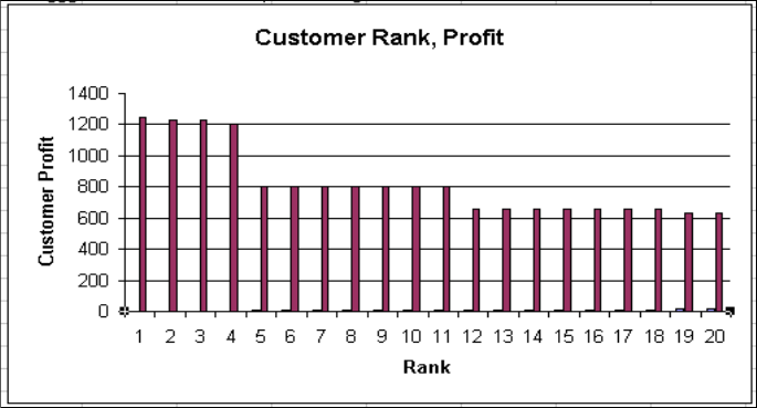
Figure 4-23 Customer profitability bar chart
4.3.2 Identify the profile of transactions concluded recently
We look at the profile of transactions from two perspectives as follows:
?
Query 1 identifies the transaction amount range which accounted for most of
the companies transactions. For how many of our transactions are worth less
9,000 dollars. This information can be used to identify spending patterns for
targeted sales campaigns.
?
Query 2 identifies the value of transactions by percentage of volumes. For
example, what is value of our transactions at the 90th percentile? This can be
used in more detailed analysis. For example, if the retailer knows that 90
percent of his sales are less than 20,000 dollars, then he can infer that
stocking many items more $20,000 may not be cost-effective. However, he
can identify products within the most common ranges.
Data
The major source for this analysis are the transactions. In our example, this data
is contained in 2 tables.
? TRANS which is the master transaction table which holds summary details of
completed transactions.
? TRANSITEM is the sales details table which holds the individual products
sold and their value by transaction.

Chapter 4. Statistics, analytic, OLAP functions in business scenarios 177
BI functions showcased
SUM, ROWNUMBER, OVER, ORDER BY
Query 1
The SQL shown in Example 4-18 can be used to generate the result set that can
then be displayed via an equi-width histogram. The transactions are assigned to
a range bucket based on the sales value of a transaction.
Example 4-18 Equi-width histogram query
WITH dt AS
(
SELECT t.transid, SUM(amount) AS trans_amt,
CASE
WHEN (SUM(amount) - 0)/((60000 - 0)/20) <= 0 THEN 0
WHEN (SUM(amount) - 0)/((60000 - 0)/20) >= 19 THEN 19
ELSE INT((SUM(amount) - 0)/((60000 - 0)/20))
END AS bucket
FROM trans t, transitem ti
WHERE t.transid=ti.transid
GROUP BY t.transid
)
SELECT bucket, COUNT(bucket) AS height,
(bucket + 1)*(60000 - 0)/20 AS max_amt
FROM dt
GROUP BY bucket
In this query, assuming a maximum transaction amount of $60,000 (based on
domain knowledge of this application), we create twenty $3000 range buckets in
the common table expression, and then count the number of transactions in each
bucket range. The CASE expression is used to assign a bucket to a particular
transaction, and the result of the common table expression is a table by
transaction of the transaction amount and the bucket it belongs to. The query
querying the result of the common table expression, then groups the rows by
bucket, counts the number of transactions in each bucket, and lists the upper
range of the bucket for these transactions.
Figure 4-24 shows the results of this query.


Chapter 4. Statistics, analytic, OLAP functions in business scenarios 179
The data and histogram shows that a significant proportion of the transactions
are less than fifteen thousand, with a peak in the six to nine thousand range. The
answer to the number of transactions worth less than 6,000 dollars is 1058. The
graph also shows that 449 transactions are less than 3000 dollars, and 609
transactions are between 3000 and 6000 dollars.
Query 2
The SQL shown in Example 4-19 can be used to generate the result set that can
then be displayed via an equi-height histogram. The bucket boundaries are
chosen so that each bucket contains approximately the same number of data
points.
Example 4-19 Equi-height histogram query
WITH dt AS
(
SELECT t.transid, SUM(amount) AS trans_amt,
ROWNUMBER() OVER (ORDER BY SUM(amount))*10/
(
SELECT COUNT(DISTINCT transid) + 1
FROM transitem
) AS bucket
FROM trans t, transitem ti
WHERE t.transid=ti.transid
GROUP BY t.transid
)
SELECT (bucket+1)*10 AS percentile, COUNT(bucket) AS b_count,
MAX(trans_amt) AS max_value
FROM dt
GROUP BY bucket
In this example we have used 10 buckets, so that 10% of the data points fall in
each bucket. The internal bucket boundaries are often referred to as the 0.1, 0.2,
..., 0.9 quantiles of the data distribution, or as the 10th, 20th, ...., 90th percentiles.
For example, Figure 4-26 shows that the 10th percentile for our data is $2840.05,
that is, 10% of transactions have a dollar value less than this amount.
In effect, the query computes the total sales amount for each of ‘n’ transactions
as trans-amt, sorts the amounts in increasing order, and assigns the number one
to the smallest transaction, two to the next largest transaction, etc. using the
ROWNUMBER() function. Multiplying these numbers by 10 (the number of
buckets), and then dividing these numbers by ‘n’ (which is computed as
COUNT(DISTINCT transid)), and rounding to the nearest integer produces the
desired bucket number for each transaction.
Figure 4-26 shows the results of this query.

180 High-Function Business Intelligence in e-business
Figure 4-26 Equi-height histogram data
As mentioned earlier, that the MAX_VALUE represents the transaction amount at
the bucket boundary.
This data is copied into Lotus 1-2-3 to create the equi-height histogram shown in
Figure 4-27. The histogram will display the max values in each bucket as the
width. It is called an “equi-height” histogram because the ranges are set to the
same height. The data in the graph has been manipulated so that the max value
is the boundary. The individual figures have had the preceding value subtracted.
Figure 4-27 Equi-height histogram
The data and histogram shows that 30% of all transactions are worth less than
7,060 dollars.
..................Content has been hidden....................
You can't read the all page of ebook, please click here login for view all page.