
132 High-Function Business Intelligence in e-business
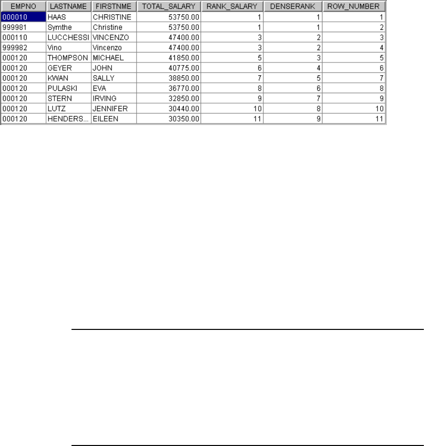
The result of this query is shown in Figure 3-11.
Figure 3-11 RANK, DENSE_RANK and ROW_NUMBER comparison
RANK and PARTITION BY example
The following is an example of using the PARTITION BY clause which allows for
subdividing the rows into partitions. It functions similar to the GROUP BY
function, but is local to the window set whereas GROUP BY is a global function.
Assume we want to find the top 4 ranking of employee salary within each
department.
We will need to use the RANK function with partition (ranking window) by
department. We will need to use a common table expression otherwise the
reference to RANK_IN_DEPT in our subselect is ambiguous.
The SQL is shown in Example 3-18.
Example 3-18 RANK & PARTITION example
WITH SALARYBYDEPT AS(
SELECT WORKDEPT, LASTNAME, FIRSTNME,SALARY,
RANK() OVER (PARTITION BY WORKDEPT ORDER BY SALARY DESC NULLS LAST)
AS RANK_IN_DEPT
FROM EMPLOYEE )
SELECT WORKDEPT, LASTNAME,FIRSTNME,SALARY, RANK_IN_DEPT
FROM SALARYBYDEPT
WHERE RANK_IN_DEPT <= 4 AND WORKDEPT IN
('A00','A11','B01','C01','D1','D11')
ORDER BY WORKDEPT, RANK_IN_DEPT, LASTNAME

Chapter 3. DB2 UDB’s statistics, analytic, and OLAP functions 133
The result of this query is shown in Figure 3-12.
Figure 3-12 PARTITION BY window results
The employee table is first partitioned by department. Then the ranking function
is applied based on highest to lowest salary within the common table expression.
Then the outer select chooses only the top 4 employees in the departments
requested and orders them by department and rank in the department. Ties in
rank are listed alphabetically.
OVER clause example
With the OVER clause it is possible to turn aggregate function like SUM, AVG,
COUNT, COUNT_BIG, CORRELATION, VARIANCE, COVARIANCE, MIN, MAX,
and STDDEV into OLAP functions. Rather than returning the aggregate of the
rows as a single value the OVER function operates on the range of rows
specified in the window and returns a single aggregate value for the range. The
following example illustrates this function.
Assume we would like to determine for each employee within a department the
percentage of that employee’s salary to the total department salary. That is if an
employee’s salary is $20,000 and the department total is $100,000 then the
employee’s percentage of the department’s salary is 20%.
Our SQL would look as shown in Example 3-19:

134 High-Function Business Intelligence in e-business
Example 3-19 OVER clause example
SELECT WORKDEPT,LASTNAME,SALARY, DECIMAL(SALARY,15,0)*100/SUM(SALARY)
OVER (PARTITION BY WORKDEPT) AS DEPT_SALARY_PERCENT
FROM EMPLOYEE
WHERE WORKDEPT IN ('A00','A11','B01','C01','D1','D11')
ORDER BY WORKDEPT, DEPT_SALARY_PERCENT DESC
The result of this query is shown in Figure 3-13. The SUM(SALARY) (sum of
salary) is ranged by the OVER (PARTITION BY... clause to only those values in
each department.
Figure 3-13 Salary as a percentage of department total salary
Chapter 3. DB2 UDB’s statistics, analytic, and OLAP functions 135
This same concept can be applied to determine product percentage of sales for
various product groups within a retail store, bank or distribution center.
ROWS and ORDER BY example
It is possible to define the rows in the window function using a window aggregate
clause when an ORDER BY clause is included in the definition. This allows the
inclusion or exclusion of ranges of values or rows within the ordering clause.
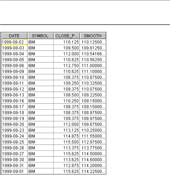
Assume we want to smooth the curve of random data similar to the 50 and 200
day moving average of stock price found on numerous stock Web sites.
The SQL and the result of the query are shown in Example 3-20 and Figure 3-14.
Example 3-20 ROWS & ORDER BY example
SELECT DATE,SYMBOL,CLOSE_PRICE,AVG(CLOSE_PRICE) OVER
(ORDER BY DATE ROWS 5 PRECEDING) AS SMOOTH
FROM STOCKTAB
WHERE SYMBOL = 'IBM'
Figure 3-14 Five day smoothing of IBM
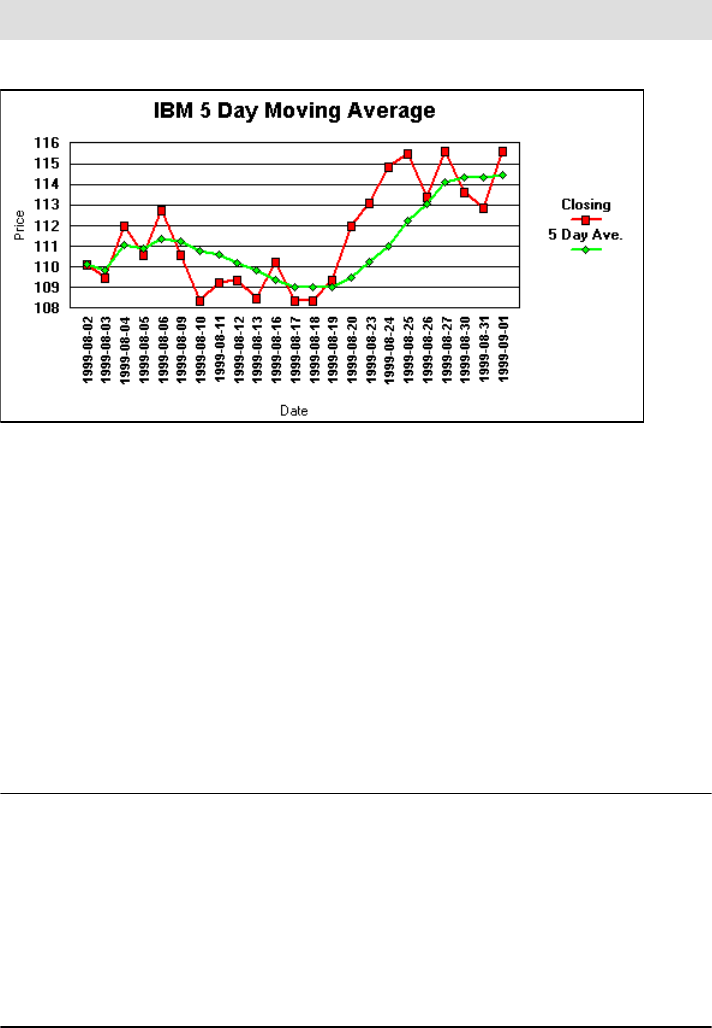
136 High-Function Business Intelligence in e-business
Figure 3-15 IBM five day moving average
The equivalent result can be calculated using the RANGE instead of ROWS.
ROWS works well in situations when the data is dense, that is, there are no
values duplicated or missing.
ROWS, RANGE, and ORDER BY example
Stock tables have the weekends missing. RANGE can be used to overcome gaps
as illustrated in the following example.
Assume we want to calculate the seven day calendar average with the intent of
taking into account the weekends. We will compare the results of ROWS versus
RANGE. The SQL is shown in Example 3-21:
Example 3-21 ROWS, RANGE & ORDER BY example
SELECT DATE, SUBSTR(DAYNAME(DATE),1,9) AS DAY_WEEK, CLOSE_PRICE,
DEC(AVG(CLOSE_PRICE) OVER (ORDER BY DATE ROWS 6 PRECEDING),7,2) AS
AVG_7_ROWS,
COUNT(CLOSE_PRICE) OVER (ORDER BY DATE ROWS 6 PRECEDING) AS COUNT_7_ROWS,
DEC(AVG(CLOSE_PRICE) OVER (ORDER BY DATE RANGE 00000006. PRECEDING),7,2) AS
AVG_7_RANGE,
COUNT(CLOSE(CLOSE_PRICE) OVER (ORDER BY DATE RANGE 00000006. PRECEDING) AS
COUNT_7_RANGE
FROM STOCKTAB
WHERE SYMBOL=’IBM’
Note: IBM stock price data is not historically accurate.
..................Content has been hidden....................
You can't read the all page of ebook, please click here login for view all page.