Personal Mobile Device (PMD)

Personal mobile device (PMD) is the term we apply to a collection of wireless devices with multimedia user interfaces such as cell phones, tablet computers, and so on. Cost is a prime concern given the consumer price for the whole product is a few hundred dollars. Although the emphasis on energy efficiency is frequently driven by the use of batteries, the need to use less expensive packaging—plastic versus ceramic—and the absence of a fan for cooling also limit total power consumption. We examine the issue of energy and power in more detail in Section 1.5. Applications on PMDs are often Web-based and media-oriented, like the Google Goggles example above. Energy and size requirements lead to use of Flash memory for storage (Chapter 2) instead of magnetic disks.

Responsiveness and predictability are key characteristics for media applications. A real-time performance requirement means a segment of the application has an absolute maximum execution time. For example, in playing a video on a PMD, the time to process each video frame is limited, since the processor must accept and process the next frame shortly. In some applications, a more nuanced requirement exists: the average time for a particular task is constrained as well as the number of instances when some maximum time is exceeded. Such approaches—sometimes called soft real-time—arise when it is possible to occasionally miss the time constraint on an event, as long as not too many are missed. Real-time performance tends to be highly application dependent.

Other key characteristics in many PMD applications are the need to minimize memory and the need to use energy efficiently. Energy efficiency is driven by both battery power and heat dissipation. The memory can be a substantial portion of the system cost, and it is important to optimize memory size in such cases. The importance of memory size translates to an emphasis on code size, since data size is dictated by the application.

Desktop Computing

The first, and probably still the largest market in dollar terms, is desktop computing. Desktop computing spans from low-end netbooks that sell for under $300 to high-end, heavily configured workstations that may sell for $2500. Since 2008, more than half of the desktop computers made each year have been battery operated laptop computers.

Throughout this range in price and capability, the desktop market tends to be driven to optimize price-performance. This combination of performance (measured primarily in terms of compute performance and graphics performance) and price of a system is what matters most to customers in this market, and hence to computer designers. As a result, the newest, highest-performance microprocessors and cost-reduced microprocessors often appear first in desktop systems (see Section 1.6 for a discussion of the issues affecting the cost of computers).

Desktop computing also tends to be reasonably well characterized in terms of applications and benchmarking, though the increasing use of Web-centric, interactive applications poses new challenges in performance evaluation.

Servers

As the shift to desktop computing occurred in the 1980s, the role of servers grew to provide larger-scale and more reliable file and computing services. Such servers have become the backbone of large-scale enterprise computing, replacing the traditional mainframe.

For servers, different characteristics are important. First, availability is critical. (We discuss availability in Section 1.7.) Consider the servers running ATM machines for banks or airline reservation systems. Failure of such server systems is far more catastrophic than failure of a single desktop, since these servers must operate seven days a week, 24 hours a day. Figure 1.3 estimates revenue costs of downtime for server applications.

Figure 1.3 Costs rounded to nearest $100,000 of an unavailable system are shown by analyzing the cost of downtime (in terms of immediately lost revenue), assuming three different levels of availability and that downtime is distributed uniformly. These data are from Kembel [2000] and were collected and analyzed by Contingency Planning Research.

A second key feature of server systems is scalability. Server systems often grow in response to an increasing demand for the services they support or an increase in functional requirements. Thus, the ability to scale up the computing capacity, the memory, the storage, and the I/O bandwidth of a server is crucial.

Finally, servers are designed for efficient throughput. That is, the overall performance of the server—in terms of transactions per minute or Web pages served per second—is what is crucial. Responsiveness to an individual request remains important, but overall efficiency and cost-effectiveness, as determined by how many requests can be handled in a unit time, are the key metrics for most servers. We return to the issue of assessing performance for different types of computing environments in Section 1.8.

Clusters/Warehouse-Scale Computers

The growth of Software as a Service (SaaS) for applications like search, social networking, video sharing, multiplayer games, online shopping, and so on has led to the growth of a class of computers called clusters. Clusters are collections of desktop computers or servers connected by local area networks to act as a single larger computer. Each node runs its own operating system, and nodes communicate using a networking protocol. The largest of the clusters are called warehouse-scale computers (WSCs), in that they are designed so that tens of thousands of servers can act as one. Chapter 6 describes this class of the extremely large computers.

Price-performance and power are critical to WSCs since they are so large. As Chapter 6 explains, 80% of the cost of a $90M warehouse is associated with power and cooling of the computers inside. The computers themselves and networking gear cost another $70M and they must be replaced every few years. When you are buying that much computing, you need to buy wisely, as a 10% improvement in price-performance means a savings of $7M (10% of $70M).

WSCs are related to servers, in that availability is critical. For example, Amazon.com had $13 billion in sales in the fourth quarter of 2010. As there are about 2200 hours in a quarter, the average revenue per hour was almost $6M. During a peak hour for Christmas shopping, the potential loss would be many times higher. As Chapter 6 explains, the difference from servers is that WSCs use redundant inexpensive components as the building blocks, relying on a software layer to catch and isolate the many failures that will happen with computing at this scale. Note that scalability for a WSC is handled by the local area network connecting the computers and not by integrated computer hardware, as in the case of servers.

Supercomputers are related to WSCs in that they are equally expensive, costing hundreds of millions of dollars, but supercomputers differ by emphasizing floating-point performance and by running large, communication-intensive batch programs that can run for weeks at a time. This tight coupling leads to use of much faster internal networks. In contrast, WSCs emphasize interactive applications, large-scale storage, dependability, and high Internet bandwidth.

Embedded Computers

Embedded computers are found in everyday machines; microwaves, washing machines, most printers, most networking switches, and all cars contain simple embedded microprocessors.

The processors in a PMD are often considered embedded computers, but we are keeping them as a separate category because PMDs are platforms that can run externally developed software and they share many of the characteristics of desktop computers. Other embedded devices are more limited in hardware and software sophistication. We use the ability to run third-party software as the dividing line between non-embedded and embedded computers.

Embedded computers have the widest spread of processing power and cost. They include 8-bit and 16-bit processors that may cost less than a dime, 32-bit microprocessors that execute 100 million instructions per second and cost under $5, and high-end processors for network switches that cost $100 and can execute billions of instructions per second. Although the range of computing power in the embedded computing market is very large, price is a key factor in the design of computers for this space. Performance requirements do exist, of course, but the primary goal is often meeting the performance need at a minimum price, rather than achieving higher performance at a higher price.

Most of this book applies to the design, use, and performance of embedded processors, whether they are off-the-shelf microprocessors or microprocessor cores that will be assembled with other special-purpose hardware. Indeed, the third edition of this book included examples from embedded computing to illustrate the ideas in every chapter.

Alas, most readers found these examples unsatisfactory, as the data that drive the quantitative design and evaluation of other classes of computers have not yet been extended well to embedded computing (see the challenges with EEMBC, for example, in Section 1.8). Hence, we are left for now with qualitative descriptions, which do not fit well with the rest of the book. As a result, in this and the prior edition we consolidated the embedded material into Appendix E. We believe a separate appendix improves the flow of ideas in the text while allowing readers to see how the differing requirements affect embedded computing.

Classes of Parallelism and Parallel Architectures

Parallelism at multiple levels is now the driving force of computer design across all four classes of computers, with energy and cost being the primary constraints. There are basically two kinds of parallelism in applications:

Computer hardware in turn can exploit these two kinds of application parallelism in four major ways:

These four ways for hardware to support the data-level parallelism and task-level parallelism go back 50 years. When Michael Flynn [1966] studied the parallel computing efforts in the 1960s, he found a simple classification whose abbreviations we still use today. He looked at the parallelism in the instruction and data streams called for by the instructions at the most constrained component of the multiprocessor, and placed all computers into one of four categories:

This taxonomy is a coarse model, as many parallel processors are hybrids of the SISD, SIMD, and MIMD classes. Nonetheless, it is useful to put a framework on the design space for the computers we will see in this book.

Instruction Set Architecture: The Myopic View of Computer Architecture

We use the term instruction set architecture (ISA) to refer to the actual programmer-visible instruction set in this book. The ISA serves as the boundary between the software and hardware. This quick review of ISA will use examples from 80x86, ARM, and MIPS to illustrate the seven dimensions of an ISA. Appendices A and K give more details on the three ISAs.

Figure 1.4 MIPS registers and usage conventions. In addition to the 32 general-purpose registers (R0–R31), MIPS has 32 floating-point registers (F0–F31) that can hold either a 32-bit single-precision number or a 64-bit double-precision number.

Figure 1.5 Subset of the instructions in MIPS64. SP = single precision; DP = double precision. Appendix A gives much more detail on MIPS64. For data, the most significant bit number is 0; least is 63.

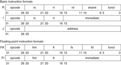
Figure 1.6 MIPS64 instruction set architecture formats. All instructions are 32 bits long. The R format is for integer register-to-register operations, such as DADDU, DSUBU, and so on. The I format is for data transfers, branches, and immediate instructions, such as LD, SD, BEQZ, and DADDIs. The J format is for jumps, the FR format for floating-point operations, and the FI format for floating-point branches.

The other challenges facing the computer architect beyond ISA design are particularly acute at the present, when the differences among instruction sets are small and when there are distinct application areas. Therefore, starting with the last edition, the bulk of instruction set material beyond this quick review is found in the appendices (see Appendices A and K).

We use a subset of MIPS64 as the example ISA in this book because it is both the dominant ISA for networking and it is an elegant example of the RISC architectures mentioned earlier, of which ARM (Advanced RISC Machine) is the most popular example. ARM processors were in 6.1 billion chips shipped in 2010, or roughly 20 times as many chips that shipped with 80x86 processors.

Genuine Computer Architecture: Designing the Organization and Hardware to Meet Goals and Functional Requirements

The implementation of a computer has two components: organization and hardware. The term organization includes the high-level aspects of a computer’s design, such as the memory system, the memory interconnect, and the design of the internal processor or CPU (central processing unit—where arithmetic, logic, branching, and data transfer are implemented). The term microarchitecture is also used instead of organization. For example, two processors with the same instruction set architectures but different organizations are the AMD Opteron and the Intel Core i7. Both processors implement the x86 instruction set, but they have very different pipeline and cache organizations.

The switch to multiple processors per microprocessor led to the term core to also be used for processor. Instead of saying multiprocessor microprocessor, the term multicore has caught on. Given that virtually all chips have multiple processors, the term central processing unit, or CPU, is fading in popularity.

Hardware refers to the specifics of a computer, including the detailed logic design and the packaging technology of the computer. Often a line of computers contains computers with identical instruction set architectures and nearly identical organizations, but they differ in the detailed hardware implementation. For example, the Intel Core i7 (see Chapter 3) and the Intel Xeon 7560 (see Chapter 5) are nearly identical but offer different clock rates and different memory systems, making the Xeon 7560 more effective for server computers.

In this book, the word architecture covers all three aspects of computer design—instruction set architecture, organization or microarchitecture, and hardware.

Computer architects must design a computer to meet functional requirements as well as price, power, performance, and availability goals. Figure 1.7 summarizes requirements to consider in designing a new computer. Often, architects also must determine what the functional requirements are, which can be a major task. The requirements may be specific features inspired by the market. Application software often drives the choice of certain functional requirements by determining how the computer will be used. If a large body of software exists for a certain instruction set architecture, the architect may decide that a new computer should implement an existing instruction set. The presence of a large market for a particular class of applications might encourage the designers to incorporate requirements that would make the computer competitive in that market. Later chapters examine many of these requirements and features in depth.

Figure 1.7 Summary of some of the most important functional requirements an architect faces. The left-hand column describes the class of requirement, while the right-hand column gives specific examples. The right-hand column also contains references to chapters and appendices that deal with the specific issues.

Architects must also be aware of important trends in both the technology and the use of computers, as such trends affect not only the future cost but also the longevity of an architecture.

Performance Trends: Bandwidth over Latency

As we shall see in Section 1.8, bandwidth or throughput is the total amount of work done in a given time, such as megabytes per second for a disk transfer. In contrast, latency or response time is the time between the start and the completion of an event, such as milliseconds for a disk access. Figure 1.9 plots the relative improvement in bandwidth and latency for technology milestones for microprocessors, memory, networks, and disks. Figure 1.10 describes the examples and milestones in more detail.

Figure 1.9 Log–log plot of bandwidth and latency milestones from Figure 1.10 relative to the first milestone. Note that latency improved 6X to 80X while bandwidth improved about 300X to 25,000X. Updated from Patterson [2004].

Figure 1.10 Performance milestones over 25 to 40 years for microprocessors, memory, networks, and disks. The microprocessor milestones are several generations of IA-32 processors, going from a 16-bit bus, microcoded 80286 to a 64-bit bus, multicore, out-of-order execution, superpipelined Core i7. Memory module milestones go from 16-bit-wide, plain DRAM to 64-bit-wide double data rate version 3 synchronous DRAM. Ethernet advanced from 10 Mbits/sec to 100 Gbits/sec. Disk milestones are based on rotation speed, improving from 3600 RPM to 15,000 RPM. Each case is best-case bandwidth, and latency is the time for a simple operation assuming no contention. Updated from Patterson [2004].

Performance is the primary differentiator for microprocessors and networks, so they have seen the greatest gains: 10,000–25,000X in bandwidth and 30–80X in latency. Capacity is generally more important than performance for memory and disks, so capacity has improved most, yet bandwidth advances of 300–1200X are still much greater than gains in latency of 6–8X.

Clearly, bandwidth has outpaced latency across these technologies and will likely continue to do so. A simple rule of thumb is that bandwidth grows by at least the square of the improvement in latency. Computer designers should plan accordingly.

Scaling of Transistor Performance and Wires

Integrated circuit processes are characterized by the feature size, which is the minimum size of a transistor or a wire in either the x or y dimension. Feature sizes have decreased from 10 microns in 1971 to 0.032 microns in 2011; in fact, we have switched units, so production in 2011 is referred to as “32 nanometers,” and 22 nanometer chips are under way. Since the transistor count per square millimeter of silicon is determined by the surface area of a transistor, the density of transistors increases quadratically with a linear decrease in feature size.

The increase in transistor performance, however, is more complex. As feature sizes shrink, devices shrink quadratically in the horizontal dimension and also shrink in the vertical dimension. The shrink in the vertical dimension requires a reduction in operating voltage to maintain correct operation and reliability of the transistors. This combination of scaling factors leads to a complex interrelationship between transistor performance and process feature size. To a first approximation, transistor performance improves linearly with decreasing feature size.

The fact that transistor count improves quadratically with a linear improvement in transistor performance is both the challenge and the opportunity for which computer architects were created! In the early days of microprocessors, the higher rate of improvement in density was used to move quickly from 4-bit, to 8-bit, to 16-bit, to 32-bit, to 64-bit microprocessors. More recently, density improvements have supported the introduction of multiple processors per chip, wider SIMD units, and many of the innovations in speculative execution and caches found in Chapters 2, 3, 4, and 5.

Although transistors generally improve in performance with decreased feature size, wires in an integrated circuit do not. In particular, the signal delay for a wire increases in proportion to the product of its resistance and capacitance. Of course, as feature size shrinks, wires get shorter, but the resistance and capacitance per unit length get worse. This relationship is complex, since both resistance and capacitance depend on detailed aspects of the process, the geometry of a wire, the loading on a wire, and even the adjacency to other structures. There are occasional process enhancements, such as the introduction of copper, which provide one-time improvements in wire delay.

In general, however, wire delay scales poorly compared to transistor performance, creating additional challenges for the designer. In the past few years, in addition to the power dissipation limit, wire delay has become a major design limitation for large integrated circuits and is often more critical than transistor switching delay. Larger and larger fractions of the clock cycle have been consumed by the propagation delay of signals on wires, but power now plays an even greater role than wire delay.

Power and Energy: A Systems Perspective

How should a system architect or a user think about performance, power, and energy? From the viewpoint of a system designer, there are three primary concerns.

First, what is the maximum power a processor ever requires? Meeting this demand can be important to ensuring correct operation. For example, if a processor attempts to draw more power than a power supply system can provide (by drawing more current than the system can supply), the result is typically a voltage drop, which can cause the device to malfunction. Modern processors can vary widely in power consumption with high peak currents; hence, they provide voltage indexing methods that allow the processor to slow down and regulate voltage within a wider margin. Obviously, doing so decreases performance.

Second, what is the sustained power consumption? This metric is widely called the thermal design power (TDP), since it determines the cooling requirement. TDP is neither peak power, which is often 1.5 times higher, nor is it the actual average power that will be consumed during a given computation, which is likely to be lower still. A typical power supply for a system is usually sized to exceed the TDP, and a cooling system is usually designed to match or exceed TDP. Failure to provide adequate cooling will allow the junction temperature in the processor to exceed its maximum value, resulting in device failure and possibly permanent damage. Modern processors provide two features to assist in managing heat, since the maximum power (and hence heat and temperature rise) can exceed the long-term average specified by the TDP. First, as the thermal temperature approaches the junction temperature limit, circuitry reduces the clock rate, thereby reducing power. Should this technique not be successful, a second thermal overload trip is activated to power down the chip.

The third factor that designers and users need to consider is energy and energy efficiency. Recall that power is simply energy per unit time: 1 watt = 1 joule per second. Which metric is the right one for comparing processors: energy or power? In general, energy is always a better metric because it is tied to a specific task and the time required for that task. In particular, the energy to execute a workload is equal to the average power times the execution time for the workload.

Thus, if we want to know which of two processors is more efficient for a given task, we should compare energy consumption (not power) for executing the task. For example, processor A may have a 20% higher average power consumption than processor B, but if A executes the task in only 70% of the time needed by B, its energy consumption will be 1.2 × 0.7 = 0.84, which is clearly better.

One might argue that in a large server or cloud, it is sufficient to consider average power, since the workload is often assumed to be infinite, but this is misleading. If our cloud were populated with processor Bs rather than As, then the cloud would do less work for the same amount of energy expended. Using energy to compare the alternatives avoids this pitfall. Whenever we have a fixed workload, whether for a warehouse-size cloud or a smartphone, comparing energy will be the right way to compare processor alternatives, as the electricity bill for the cloud and the battery lifetime for the smartphone are both determined by the energy consumed.

When is power consumption a useful measure? The primary legitimate use is as a constraint: for example, a chip might be limited to 100 watts. It can be used as a metric if the workload is fixed, but then it’s just a variation of the true metric of energy per task.

Energy and Power within a Microprocessor

For CMOS chips, the traditional primary energy consumption has been in switching transistors, also called dynamic energy. The energy required per transistor is proportional to the product of the capacitive load driven by the transistor and the square of the voltage:

This equation is the energy of pulse of the logic transition of 0→1→0 or 1→0→1. The energy of a single transition (0→1 or 1→0) is then:

The power required per transistor is just the product of the energy of a transition multiplied by the frequency of transitions:

For a fixed task, slowing clock rate reduces power, but not energy.

Clearly, dynamic power and energy are greatly reduced by lowering the voltage, so voltages have dropped from 5V to just under 1V in 20 years. The capacitive load is a function of the number of transistors connected to an output and the technology, which determines the capacitance of the wires and the transistors.

As we move from one process to the next, the increase in the number of transistors switching and the frequency with which they switch dominate the decrease in load capacitance and voltage, leading to an overall growth in power consumption and energy. The first microprocessors consumed less than a watt and the first 32-bit microprocessors (like the Intel 80386) used about 2 watts, while a 3.3 GHz Intel Core i7 consumes 130 watts. Given that this heat must be dissipated from a chip that is about 1.5 cm on a side, we have reached the limit of what can be cooled by air.

Given the equation above, you would expect clock frequency growth to slow down if we can’t reduce voltage or increase power per chip. Figure 1.11 shows that this has indeed been the case since 2003, even for the microprocessors in Figure 1.1 that were the highest performers each year. Note that this period of flat clock rates corresponds to the period of slow performance improvement range in Figure 1.1.

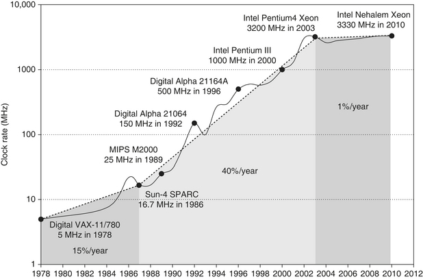
Figure 1.11 Growth in clock rate of microprocessors in Figure 1.1. Between 1978 and 1986, the clock rate improved less than 15% per year while performance improved by 25% per year. During the “renaissance period” of 52% performance improvement per year between 1986 and 2003, clock rates shot up almost 40% per year. Since then, the clock rate has been nearly flat, growing at less than 1% per year, while single processor performance improved at less than 22% per year.

Distributing the power, removing the heat, and preventing hot spots have become increasingly difficult challenges. Power is now the major constraint to using transistors; in the past, it was raw silicon area. Hence, modern microprocessors offer many techniques to try to improve energy efficiency despite flat clock rates and constant supply voltages:

Figure 1.12 Energy savings for a server using an AMD Opteron microprocessor, 8 GB of DRAM, and one ATA disk. At 1.8 GHz, the server can only handle up to two-thirds of the workload without causing service level violations, and, at 1.0 GHz, it can only safely handle one-third of the workload. (Figure 5.11 in Barroso and Hölzle [2009].)

Although dynamic power is traditionally thought of as the primary source of power dissipation in CMOS, static power is becoming an important issue because leakage current flows even when a transistor is off:

That is, static power is proportional to number of devices.

Thus, increasing the number of transistors increases power even if they are idle, and leakage current increases in processors with smaller transistor sizes. As a result, very low power systems are even turning off the power supply (power gating) to inactive modules to control loss due to leakage. In 2011, the goal for leakage is 25% of the total power consumption, with leakage in high-performance designs sometimes far exceeding that goal. Leakage can be as high as 50% for such chips, in part because of the large SRAM caches that need power to maintain the storage values. (The S in SRAM is for static.) The only hope to stop leakage is to turn off power to subsets of the chips.

Finally, because the processor is just a portion of the whole energy cost of a system, it can make sense to use a faster, less energy-efficient processor to allow the rest of the system to go into a sleep mode. This strategy is known as race-to-halt.

The importance of power and energy has increased the scrutiny on the efficiency of an innovation, so the primary evaluation now is tasks per joule or performance per watt as opposed to performance per mm² of silicon. This new metric affects approaches to parallelism, as we shall see in Chapters 4 and 5.

The Impact of Time, Volume, and Commoditization

The cost of a manufactured computer component decreases over time even without major improvements in the basic implementation technology. The underlying principle that drives costs down is the learning curve—manufacturing costs decrease over time. The learning curve itself is best measured by change in yield—the percentage of manufactured devices that survives the testing procedure. Whether it is a chip, a board, or a system, designs that have twice the yield will have half the cost.

Understanding how the learning curve improves yield is critical to projecting costs over a product’s life. One example is that the price per megabyte of DRAM has dropped over the long term. Since DRAMs tend to be priced in close relationship to cost—with the exception of periods when there is a shortage or an oversupply—price and cost of DRAM track closely.

Microprocessor prices also drop over time, but, because they are less standardized than DRAMs, the relationship between price and cost is more complex. In a period of significant competition, price tends to track cost closely, although microprocessor vendors probably rarely sell at a loss.

Volume is a second key factor in determining cost. Increasing volumes affect cost in several ways. First, they decrease the time needed to get down the learning curve, which is partly proportional to the number of systems (or chips) manufactured. Second, volume decreases cost, since it increases purchasing and manufacturing efficiency. As a rule of thumb, some designers have estimated that cost decreases about 10% for each doubling of volume. Moreover, volume decreases the amount of development cost that must be amortized by each computer, thus allowing cost and selling price to be closer.

Commodities are products that are sold by multiple vendors in large volumes and are essentially identical. Virtually all the products sold on the shelves of grocery stores are commodities, as are standard DRAMs, Flash memory, disks, monitors, and keyboards. In the past 25 years, much of the personal computer industry has become a commodity business focused on building desktop and laptop computers running Microsoft Windows.

Because many vendors ship virtually identical products, the market is highly competitive. Of course, this competition decreases the gap between cost and selling price, but it also decreases cost. Reductions occur because a commodity market has both volume and a clear product definition, which allows multiple suppliers to compete in building components for the commodity product. As a result, the overall product cost is lower because of the competition among the suppliers of the components and the volume efficiencies the suppliers can achieve. This rivalry has led to the low end of the computer business being able to achieve better price-performance than other sectors and yielded greater growth at the low end, although with very limited profits (as is typical in any commodity business).

Cost of an Integrated Circuit

Why would a computer architecture book have a section on integrated circuit costs? In an increasingly competitive computer marketplace where standard parts—disks, Flash memory, DRAMs, and so on—are becoming a significant portion of any system’s cost, integrated circuit costs are becoming a greater portion of the cost that varies between computers, especially in the high-volume, cost-sensitive portion of the market. Indeed, with personal mobile devices’ increasing reliance of whole systems on a chip (SOC), the cost of the integrated circuits is much of the cost of the PMD. Thus, computer designers must understand the costs of chips to understand the costs of current computers.

Although the costs of integrated circuits have dropped exponentially, the basic process of silicon manufacture is unchanged: A wafer is still tested and chopped into dies that are packaged (see Figures 1.13, 1.14, and 1.15). Thus, the cost of a packaged integrated circuit is

In this section, we focus on the cost of dies, summarizing the key issues in testing and packaging at the end.

Figure 1.13 Photograph of an Intel Core i7 microprocessor die, which is evaluated in Chapters 2 through 5. The dimensions are 18.9 mm by 13.6 mm (257 mm2) in a 45 nm process. (Courtesy Intel.)

Figure 1.14 Floorplan of Core i7 die in Figure 1.13 on left with close-up of floorplan of second core on right.

Figure 1.15 This 300 mm wafer contains 280 full Sandy Bridge dies, each 20.7 by 10.5 mm in a 32 nm process. (Sandy Bridge is Intel’s successor to Nehalem used in the Core i7.) At 216 mm2, the formula for dies per wafer estimates 282. (Courtesy Intel.)

Learning how to predict the number of good chips per wafer requires first learning how many dies fit on a wafer and then learning how to predict the percentage of those that will work. From there it is simple to predict cost:

The most interesting feature of this first term of the chip cost equation is its sensitivity to die size, shown below.

The number of dies per wafer is approximately the area of the wafer divided by the area of the die. It can be more accurately estimated by

The first term is the ratio of wafer area (πr²) to die area. The second compensates for the “square peg in a round hole” problem—rectangular dies near the periphery of round wafers. Dividing the circumference (πd) by the diagonal of a square die is approximately the number of dies along the edge.

However, this formula only gives the maximum number of dies per wafer. The critical question is: What is the fraction of good dies on a wafer, or the die yield? A simple model of integrated circuit yield, which assumes that defects are randomly distributed over the wafer and that yield is inversely proportional to the complexity of the fabrication process, leads to the following:

This Bose–Einstein formula is an empirical model developed by looking at the yield of many manufacturing lines [Sydow 2006]. Wafer yield accounts for wafers that are completely bad and so need not be tested. For simplicity, we’ll just assume the wafer yield is 100%. Defects per unit area is a measure of the random manufacturing defects that occur. In 2010, the value was typically 0.1 to 0.3 defects per square inch, or 0.016 to 0.057 defects per square centimeter, for a 40 nm process, as it depends on the maturity of the process (recall the learning curve, mentioned earlier). Finally, N is a parameter called the process-complexity factor, a measure of manufacturing difficulty. For 40 nm processes in 2010, N ranged from 11.5 to 15.5.

The bottom line is the number of good dies per wafer, which comes from multiplying dies per wafer by die yield to incorporate the effects of defects. The examples above predict about 109 good 2.25 cm² dies from the 300 mm wafer and 424 good 1.00 cm² dies. Many microprocessors fall between these two sizes. Low-end embedded 32-bit processors are sometimes as small as 0.10 cm², and processors used for embedded control (in printers, microwaves, and so on) are often less than 0.04 cm².

Given the tremendous price pressures on commodity products such as DRAM and SRAM, designers have included redundancy as a way to raise yield. For a number of years, DRAMs have regularly included some redundant memory cells, so that a certain number of flaws can be accommodated. Designers have used similar techniques in both standard SRAMs and in large SRAM arrays used for caches within microprocessors. Obviously, the presence of redundant entries can be used to boost the yield significantly.

Processing of a 300 mm (12-inch) diameter wafer in a leading-edge technology cost between $5000 and $6000 in 2010. Assuming a processed wafer cost of $5500, the cost of the 1.00 cm² die would be around $13, but the cost per die of the 2.25 cm² die would be about $51, or almost four times the cost for a die that is a little over twice as large.

What should a computer designer remember about chip costs? The manufacturing process dictates the wafer cost, wafer yield, and defects per unit area, so the sole control of the designer is die area. In practice, because the number of defects per unit area is small, the number of good dies per wafer, and hence the cost per die, grows roughly as the square of the die area. The computer designer affects die size, and hence cost, both by what functions are included on or excluded from the die and by the number of I/O pins.

Before we have a part that is ready for use in a computer, the die must be tested (to separate the good dies from the bad), packaged, and tested again after packaging. These steps all add significant costs.

The above analysis has focused on the variable costs of producing a functional die, which is appropriate for high-volume integrated circuits. There is, however, one very important part of the fixed costs that can significantly affect the cost of an integrated circuit for low volumes (less than 1 million parts), namely, the cost of a mask set. Each step in the integrated circuit process requires a separate mask. Thus, for modern high-density fabrication processes with four to six metal layers, mask costs exceed $1M. Obviously, this large fixed cost affects the cost of prototyping and debugging runs and, for small-volume production, can be a significant part of the production cost. Since mask costs are likely to continue to increase, designers may incorporate reconfigurable logic to enhance the flexibility of a part or choose to use gate arrays (which have fewer custom mask levels) and thus reduce the cost implications of masks.

Cost versus Price

With the commoditization of computers, the margin between the cost to manufacture a product and the price the product sells for has been shrinking. Those margins pay for a company’s research and development (R&D), marketing, sales, manufacturing equipment maintenance, building rental, cost of financing, pretax profits, and taxes. Many engineers are surprised to find that most companies spend only 4% (in the commodity PC business) to 12% (in the high-end server business) of their income on R&D, which includes all engineering.

Cost of Manufacturing versus Cost of Operation

For the first four editions of this book, cost meant the cost to build a computer and price meant price to purchase a computer. With the advent of warehouse-scale computers, which contain tens of thousands of servers, the cost to operate the computers is significant in addition to the cost of purchase.

As Chapter 6 shows, the amortized purchase price of servers and networks is just over 60% of the monthly cost to operate a warehouse-scale computer, assuming a short lifetime of the IT equipment of 3 to 4 years. About 30% of the monthly operational costs are for power use and the amortized infrastructure to distribute power and to cool the IT equipment, despite this infrastructure being amortized over 10 years. Thus, to lower operational costs in a warehouse-scale computer, computer architects need to use energy efficiently.

Benchmarks

The best choice of benchmarks to measure performance is real applications, such as Google Goggles from Section 1.1. Attempts at running programs that are much simpler than a real application have led to performance pitfalls. Examples include:

Kernels, which are small, key pieces of real applications

Toy programs, which are 100-line programs from beginning programming assignments, such as quicksort

Synthetic benchmarks, which are fake programs invented to try to match the profile and behavior of real applications, such as Dhrystone

All three are discredited today, usually because the compiler writer and architect can conspire to make the computer appear faster on these stand-in programs than on real applications. Depressingly for your authors—who dropped the fallacy about using synthetic programs to characterize performance in the fourth edition of this book since we thought computer architects agreed it was disreputable—the synthetic program Dhrystone is still the most widely quoted benchmark for embedded processors!

Another issue is the conditions under which the benchmarks are run. One way to improve the performance of a benchmark has been with benchmark-specific flags; these flags often caused transformations that would be illegal on many programs or would slow down performance on others. To restrict this process and increase the significance of the results, benchmark developers often require the vendor to use one compiler and one set of flags for all the programs in the same language (C++ or C). In addition to the question of compiler flags, another question is whether source code modifications are allowed. There are three different approaches to addressing this question:

The key issue that benchmark designers face in deciding to allow modification of the source is whether such modifications will reflect real practice and provide useful insight to users, or whether such modifications simply reduce the accuracy of the benchmarks as predictors of real performance.

To overcome the danger of placing too many eggs in one basket, collections of benchmark applications, called benchmark suites, are a popular measure of performance of processors with a variety of applications. Of course, such suites are only as good as the constituent individual benchmarks. Nonetheless, a key advantage of such suites is that the weakness of any one benchmark is lessened by the presence of the other benchmarks. The goal of a benchmark suite is that it will characterize the relative performance of two computers, particularly for programs not in the suite that customers are likely to run.

A cautionary example is the Electronic Design News Embedded Microprocessor Benchmark Consortium (or EEMBC, pronounced “embassy”) benchmarks. It is a set of 41 kernels used to predict performance of different embedded applications: automotive/industrial, consumer, networking, office automation, and telecommunications. EEMBC reports unmodified performance and “full fury” performance, where almost anything goes. Because these benchmarks use kernels, and because of the reporting options, EEMBC does not have the reputation of being a good predictor of relative performance of different embedded computers in the field. This lack of success is why Dhrystone, which EEMBC was trying to replace, is still used.

One of the most successful attempts to create standardized benchmark application suites has been the SPEC (Standard Performance Evaluation Corporation), which had its roots in efforts in the late 1980s to deliver better benchmarks for workstations. Just as the computer industry has evolved over time, so has the need for different benchmark suites, and there are now SPEC benchmarks to cover many application classes. All the SPEC benchmark suites and their reported results are found at www.spec.org.

Although we focus our discussion on the SPEC benchmarks in many of the following sections, many benchmarks have also been developed for PCs running the Windows operating system.

Desktop Benchmarks

Desktop benchmarks divide into two broad classes: processor-intensive benchmarks and graphics-intensive benchmarks, although many graphics benchmarks include intensive processor activity. SPEC originally created a benchmark set focusing on processor performance (initially called SPEC89), which has evolved into its fifth generation: SPEC CPU2006, which follows SPEC2000, SPEC95 SPEC92, and SPEC89. SPEC CPU2006 consists of a set of 12 integer benchmarks (CINT2006) and 17 floating-point benchmarks (CFP2006). Figure 1.16 describes the current SPEC benchmarks and their ancestry.

Figure 1.16 SPEC2006 programs and the evolution of the SPEC benchmarks over time, with integer programs above the line and floating-point programs below the line. Of the 12 SPEC2006 integer programs, 9 are written in C, and the rest in C++. For the floating-point programs, the split is 6 in Fortran, 4 in C++, 3 in C, and 4 in mixed C and Fortran. The figure shows all 70 of the programs in the 1989, 1992, 1995, 2000, and 2006 releases. The benchmark descriptions on the left are for SPEC2006 only and do not apply to earlier versions. Programs in the same row from different generations of SPEC are generally not related; for example, fpppp is not a CFD code like bwaves. Gcc is the senior citizen of the group. Only 3 integer programs and 3 floating-point programs survived three or more generations. Note that all the floating-point programs are new for SPEC2006. Although a few are carried over from generation to generation, the version of the program changes and either the input or the size of the benchmark is often changed to increase its running time and to avoid perturbation in measurement or domination of the execution time by some factor other than CPU time.

SPEC benchmarks are real programs modified to be portable and to minimize the effect of I/O on performance. The integer benchmarks vary from part of a C compiler to a chess program to a quantum computer simulation. The floating-point benchmarks include structured grid codes for finite element modeling, particle method codes for molecular dynamics, and sparse linear algebra codes for fluid dynamics. The SPEC CPU suite is useful for processor benchmarking for both desktop systems and single-processor servers. We will see data on many of these programs throughout this text. However, note that these programs share little with programming languages and environments and the Google Goggles application that Section 1.1 describes. Seven use C++, eight use C, and nine use Fortran! They are even statically linked, and the applications themselves are dull. It’s not clear that SPECINT2006 and SPECFP2006 capture what is exciting about computing in the 21st century.

In Section 1.11, we describe pitfalls that have occurred in developing the SPEC benchmark suite, as well as the challenges in maintaining a useful and predictive benchmark suite.

SPEC CPU2006 is aimed at processor performance, but SPEC offers many other benchmarks.

Reporting Performance Results

The guiding principle of reporting performance measurements should be reproducibility—list everything another experimenter would need to duplicate the results. A SPEC benchmark report requires an extensive description of the computer and the compiler flags, as well as the publication of both the baseline and optimized results. In addition to hardware, software, and baseline tuning parameter descriptions, a SPEC report contains the actual performance times, shown both in tabular form and as a graph. A TPC benchmark report is even more complete, since it must include results of a benchmarking audit and cost information. These reports are excellent sources for finding the real costs of computing systems, since manufacturers compete on high performance and cost-performance.

Summarizing Performance Results

In practical computer design, you must evaluate myriad design choices for their relative quantitative benefits across a suite of benchmarks believed to be relevant. Likewise, consumers trying to choose a computer will rely on performance measurements from benchmarks, which hopefully are similar to the user’s applications. In both cases, it is useful to have measurements for a suite of benchmarks so that the performance of important applications is similar to that of one or more benchmarks in the suite and that variability in performance can be understood. In the ideal case, the suite resembles a statistically valid sample of the application space, but such a sample requires more benchmarks than are typically found in most suites and requires a randomized sampling, which essentially no benchmark suite uses.

Once we have chosen to measure performance with a benchmark suite, we would like to be able to summarize the performance results of the suite in a single number. A straightforward approach to computing a summary result would be to compare the arithmetic means of the execution times of the programs in the suite. Alas, some SPEC programs take four times longer than others do, so those programs would be much more important if the arithmetic mean were the single number used to summarize performance. An alternative would be to add a weighting factor to each benchmark and use the weighted arithmetic mean as the single number to summarize performance. The problem would then be how to pick weights; since SPEC is a consortium of competing companies, each company might have their own favorite set of weights, which would make it hard to reach consensus. One approach is to use weights that make all programs execute an equal time on some reference computer, but this biases the results to the performance characteristics of the reference computer.

Rather than pick weights, we could normalize execution times to a reference computer by dividing the time on the reference computer by the time on the computer being rated, yielding a ratio proportional to performance. SPEC uses this approach, calling the ratio the SPECRatio. It has a particularly useful property that it matches the way we compare computer performance throughout this text—namely, comparing performance ratios. For example, suppose that the SPECRatio of computer A on a benchmark was 1.25 times higher than computer B; then we would know:

Notice that the execution times on the reference computer drop out and the choice of the reference computer is irrelevant when the comparisons are made as a ratio, which is the approach we consistently use. Figure 1.17 gives an example.

Figure 1.17 SPECfp2000 execution times (in seconds) for the Sun Ultra 5—the reference computer of SPEC2000—and execution times and SPECRatios for the AMD Opteron and Intel Itanium 2. (SPEC2000 multiplies the ratio of execution times by 100 to remove the decimal point from the result, so 20.86 is reported as 2086.) The final two columns show the ratios of execution times and SPECRatios. This figure demonstrates the irrelevance of the reference computer in relative performance. The ratio of the execution times is identical to the ratio of the SPECRatios, and the ratio of the geometric means (27.12/20.86 = 1.30) is identical to the geometric mean of the ratios (1.30).

Because a SPECRatio is a ratio rather than an absolute execution time, the mean must be computed using the geometric mean. (Since SPECRatios have no units, comparing SPECRatios arithmetically is meaningless.) The formula is

In the case of SPEC, sample_i is the SPECRatio for program i. Using the geometric mean ensures two important properties:

Hence, the motivations to use the geometric mean are substantial, especially when we use performance ratios to make comparisons.

Take Advantage of Parallelism

Taking advantage of parallelism is one of the most important methods for improving performance. Every chapter in this book has an example of how performance is enhanced through the exploitation of parallelism. We give three brief examples here, which are expounded on in later chapters.

Our first example is the use of parallelism at the system level. To improve the throughput performance on a typical server benchmark, such as SPECWeb or TPC-C, multiple processors and multiple disks can be used. The workload of handling requests can then be spread among the processors and disks, resulting in improved throughput. Being able to expand memory and the number of processors and disks is called scalability, and it is a valuable asset for servers. Spreading of data across many disks for parallel reads and writes enables data-level parallelism. SPECWeb also relies on request-level parallelism to use many processors while TPC-C uses thread-level parallelism for faster processing of database queries.

At the level of an individual processor, taking advantage of parallelism among instructions is critical to achieving high performance. One of the simplest ways to do this is through pipelining. (It is explained in more detail in Appendix C and is a major focus of Chapter 3.) The basic idea behind pipelining is to overlap instruction execution to reduce the total time to complete an instruction sequence. A key insight that allows pipelining to work is that not every instruction depends on its immediate predecessor, so executing the instructions completely or partially in parallel may be possible. Pipelining is the best-known example of instruction-level parallelism.

Parallelism can also be exploited at the level of detailed digital design. For example, set-associative caches use multiple banks of memory that are typically searched in parallel to find a desired item. Modern ALUs (arithmetic-logical units) use carry-lookahead, which uses parallelism to speed the process of computing sums from linear to logarithmic in the number of bits per operand. These are more examples of data-level parallelism.

Principle of Locality

Important fundamental observations have come from properties of programs. The most important program property that we regularly exploit is the principle of locality: Programs tend to reuse data and instructions they have used recently. A widely held rule of thumb is that a program spends 90% of its execution time in only 10% of the code. An implication of locality is that we can predict with reasonable accuracy what instructions and data a program will use in the near future based on its accesses in the recent past. The principle of locality also applies to data accesses, though not as strongly as to code accesses.

Two different types of locality have been observed. Temporal locality states that recently accessed items are likely to be accessed in the near future. Spatial locality says that items whose addresses are near one another tend to be referenced close together in time. We will see these principles applied in Chapter 2.

Focus on the Common Case

Perhaps the most important and pervasive principle of computer design is to focus on the common case: In making a design trade-off, favor the frequent case over the infrequent case. This principle applies when determining how to spend resources, since the impact of the improvement is higher if the occurrence is frequent.

Focusing on the common case works for power as well as for resource allocation and performance. The instruction fetch and decode unit of a processor may be used much more frequently than a multiplier, so optimize it first. It works on dependability as well. If a database server has 50 disks for every processor, storage dependability will dominate system dependability.

In addition, the frequent case is often simpler and can be done faster than the infrequent case. For example, when adding two numbers in the processor, we can expect overflow to be a rare circumstance and can therefore improve performance by optimizing the more common case of no overflow. This emphasis may slow down the case when overflow occurs, but if that is rare then overall performance will be improved by optimizing for the normal case.

We will see many cases of this principle throughout this text. In applying this simple principle, we have to decide what the frequent case is and how much performance can be improved by making that case faster. A fundamental law, called Amdahl’s law, can be used to quantify this principle.

Amdahl’s Law

The performance gain that can be obtained by improving some portion of a computer can be calculated using Amdahl’s law. Amdahl’s law states that the performance improvement to be gained from using some faster mode of execution is limited by the fraction of the time the faster mode can be used.

Amdahl’s law defines the speedup that can be gained by using a particular feature. What is speedup? Suppose that we can make an enhancement to a computer that will improve performance when it is used. Speedup is the ratio:

Alternatively,

Speedup tells us how much faster a task will run using the computer with the enhancement as opposed to the original computer.

Amdahl’s law gives us a quick way to find the speedup from some enhancement, which depends on two factors:

The execution time using the original computer with the enhanced mode will be the time spent using the unenhanced portion of the computer plus the time spent using the enhancement:

The overall speedup is the ratio of the execution times:

Amdahl’s law expresses the law of diminishing returns: The incremental improvement in speedup gained by an improvement of just a portion of the computation diminishes as improvements are added. An important corollary of Amdahl’s law is that if an enhancement is only usable for a fraction of a task then we can’t speed up the task by more than the reciprocal of 1 minus that fraction.

A common mistake in applying Amdahl’s law is to confuse “fraction of time converted to use an enhancement” and “fraction of time after enhancement is in use.” If, instead of measuring the time that we could use the enhancement in a computation, we measure the time after the enhancement is in use, the results will be incorrect!

Amdahl’s law can serve as a guide to how much an enhancement will improve performance and how to distribute resources to improve cost-performance. The goal, clearly, is to spend resources proportional to where time is spent. Amdahl’s law is particularly useful for comparing the overall system performance of two alternatives, but it can also be applied to compare two processor design alternatives, as the following example shows.

Amdahl’s law is applicable beyond performance. Let’s redo the reliability example from page 35 after improving the reliability of the power supply via redundancy from 200,000-hour to 830,000,000-hour MTTF, or 4150X better.

In the examples above, we needed the fraction consumed by the new and improved version; often it is difficult to measure these times directly. In the next section, we will see another way of doing such comparisons based on the use of an equation that decomposes the CPU execution time into three separate components. If we know how an alternative affects these three components, we can determine its overall performance. Furthermore, it is often possible to build simulators that measure these components before the hardware is actually designed.

The Processor Performance Equation

Essentially all computers are constructed using a clock running at a constant rate. These discrete time events are called ticks, clock ticks, clock periods, clocks, cycles, or clock cycles. Computer designers refer to the time of a clock period by its duration (e.g., 1 ns) or by its rate (e.g., 1 GHz). CPU time for a program can then be expressed two ways:

or

In addition to the number of clock cycles needed to execute a program, we can also count the number of instructions executed—the instruction path length or instruction count (IC). If we know the number of clock cycles and the instruction count, we can calculate the average number of clock cycles per instruction (CPI). Because it is easier to work with, and because we will deal with simple processors in this chapter, we use CPI. Designers sometimes also use instructions per clock (IPC), which is the inverse of CPI.

CPI is computed as

This processor figure of merit provides insight into different styles of instruction sets and implementations, and we will use it extensively in the next four chapters.

By transposing the instruction count in the above formula, clock cycles can be defined as IC × CPI. This allows us to use CPI in the execution time formula:

Expanding the first formula into the units of measurement shows how the pieces fit together:

As this formula demonstrates, processor performance is dependent upon three characteristics: clock cycle (or rate), clock cycles per instruction, and instruction count. Furthermore, CPU time is equally dependent on these three characteristics; for example, a 10% improvement in any one of them leads to a 10% improvement in CPU time.

Unfortunately, it is difficult to change one parameter in complete isolation from others because the basic technologies involved in changing each characteristic are interdependent:

Clock cycle time—Hardware technology and organization

CPI—Organization and instruction set architecture

Instruction count—Instruction set architecture and compiler technology

Luckily, many potential performance improvement techniques primarily improve one component of processor performance with small or predictable impacts on the other two.

Sometimes it is useful in designing the processor to calculate the number of total processor clock cycles as

where IC_i represents the number of times instruction i is executed in a program and CPI_i represents the average number of clocks per instruction for instruction i. This form can be used to express CPU time as

and overall CPI as

The latter form of the CPI calculation uses each individual CPI_i and the fraction of occurrences of that instruction in a program (i.e., IC_i ÷ Instruction count). CPI_i should be measured and not just calculated from a table in the back of a reference manual since it must include pipeline effects, cache misses, and any other memory system inefficiencies.

Consider our performance example on page 47, here modified to use measurements of the frequency of the instructions and of the instruction CPI values, which, in practice, are obtained by simulation or by hardware instrumentation.

It is often possible to measure the constituent parts of the processor performance equation. This is a key advantage of using the processor performance equation versus Amdahl’s law in the previous example. In particular, it may be difficult to measure things such as the fraction of execution time for which a set of instructions is responsible. In practice, this would probably be computed by summing the product of the instruction count and the CPI for each of the instructions in the set. Since the starting point is often individual instruction count and CPI measurements, the processor performance equation is incredibly useful.

To use the processor performance equation as a design tool, we need to be able to measure the various factors. For an existing processor, it is easy to obtain the execution time by measurement, and we know the default clock speed. The challenge lies in discovering the instruction count or the CPI. Most new processors include counters for both instructions executed and for clock cycles. By periodically monitoring these counters, it is also possible to attach execution time and instruction count to segments of the code, which can be helpful to programmers trying to understand and tune the performance of an application. Often, a designer or programmer will want to understand performance at a more fine-grained level than what is available from the hardware counters. For example, they may want to know why the CPI is what it is. In such cases, simulation techniques used are like those for processors that are being designed.

Techniques that help with energy efficiency, such as dynamic voltage frequency scaling and overclocking (see Section 1.5), make this equation harder to use, since the clock speed may vary while we measure the program. A simple approach is to turn off those features to make the results reproducible. Fortunately, as performance and energy efficiency are often highly correlated—taking less time to run a program generally saves energy—it’s probably safe to consider performance without worrying about the impact of DVFS or overclocking on the results.

Case Study 1: Chip Fabrication Cost

Concepts illustrated by this case study

Fabrication Cost

Fabrication Yield

Defect Tolerance through Redundancy

There are many factors involved in the price of a computer chip. New, smaller technology gives a boost in performance and a drop in required chip area. In the smaller technology, one can either keep the small area or place more hardware on the chip in order to get more functionality. In this case study, we explore how different design decisions involving fabrication technology, area, and redundancy affect the cost of chips.

1.1 [10/10] <1.6> Figure 1.22 gives the relevant chip statistics that influence the cost of several current chips. In the next few exercises, you will be exploring the effect of different possible design decisions for the IBM Power5.

Figure 1.22 Manufacturing cost factors for several modern processors.

a. [10] <1.6> What is the yield for the IBM Power5?

b. [10] <1.6> Why does the IBM Power5 have a lower defect rate than the Niagara and Opteron?

1.2 [20/20/20/20] <1.6> It costs $1 billion to build a new fabrication facility. You will be selling a range of chips from that factory, and you need to decide how much capacity to dedicate to each chip. Your Woods chip will be 150 mm2 and will make a profit of $20 per defect-free chip. Your Markon chip will be 250 mm2 and will make a profit of $25 per defect-free chip. Your fabrication facility will be identical to that for the Power5. Each wafer has a 300 mm diameter.

a. [20] <1.6> How much profit do you make on each wafer of Woods chip?

b. [20] <1.6> How much profit do you make on each wafer of Markon chip?

c. [20] <1.6> Which chip should you produce in this facility?

d. [20] <1.6> What is the profit on each new Power5 chip? If your demand is 50,000 Woods chips per month and 25,000 Markon chips per month, and your facility can fabricate 150 wafers a month, how many wafers should you make of each chip?

1.3 [20/20] <1.6> Your colleague at AMD suggests that, since the yield is so poor, you might make chips more cheaply if you placed an extra core on the die and only threw out chips on which both processors had failed. We will solve this exercise by viewing the yield as a probability of no defects occurring in a certain area given the defect rate. Calculate probabilities based on each Opteron core separately (this may not be entirely accurate, since the yield equation is based on empirical evidence rather than a mathematical calculation relating the probabilities of finding errors in different portions of the chip).

a. [20] <1.6> What is the probability that a defect will occur on no more than one of the two processor cores?

b. [20] <1.6> If the old chip cost $20 dollars per chip, what will the cost be of the new chip, taking into account the new area and yield?

Case Study 2: Power Consumption in Computer Systems

Concepts illustrated by this case study

Amdahl’s Law

Redundancy

MTTF

Power Consumption

Power consumption in modern systems is dependent on a variety of factors, including the chip clock frequency, efficiency, disk drive speed, disk drive utilization, and DRAM. The following exercises explore the impact on power that different design decisions and use scenarios have.

1.4 [20/10/20] <1.5> Figure 1.23 presents the power consumption of several computer system components. In this exercise, we will explore how the hard drive affects power consumption for the system.

Figure 1.23 Power consumption of several computer components.

a. [20] <1.5> Assuming the maximum load for each component, and a power supply efficiency of 80%, what wattage must the server’s power supply deliver to a system with an Intel Pentium 4 chip, 2 GB 240-pin Kingston DRAM, and one 7200 rpm hard drive?

b. [10] <1.5> How much power will the 7200 rpm disk drive consume if it is idle roughly 60% of the time?

c. [20] <1.5> Given that the time to read data off a 7200 rpm disk drive will be roughly 75% of a 5400 rpm disk, at what idle time of the 7200 rpm disk will the power consumption be equal, on average, for the two disks?

1.5 [10/10/20] <1.5> One critical factor in powering a server farm is cooling. If heat is not removed from the computer efficiently, the fans will blow hot air back onto the computer, not cold air. We will look at how different design decisions affect the necessary cooling, and thus the price, of a system. Use Figure 1.23 for your power calculations.

a. [10] <1.5> A cooling door for a rack costs $4000 and dissipates 14 KW (into the room; additional cost is required to get it out of the room). How many servers with an Intel Pentium 4 processor, 1 GB 240-pin DRAM, and a single 7200 rpm hard drive can you cool with one cooling door?

b. [10] <1.5> You are considering providing fault tolerance for your hard drive. RAID 1 doubles the number of disks (see Chapter 6). Now how many systems can you place on a single rack with a single cooler?

c. [20] <1.5> Typical server farms can dissipate a maximum of 200 W per square foot. Given that a server rack requires 11 square feet (including front and back clearance), how many servers from part (a) can be placed on a single rack, and how many cooling doors are required?

1.6 [Discussion] <1.8> Figure 1.24 gives a comparison of power and performance for several benchmarks comparing two servers: Sun Fire T2000 (which uses Niagara) and IBM x346 (using Intel Xeon processors). This information was reported on a Sun Web site. There are two pieces of information reported: power and speed on two benchmarks. For the results shown, the Sun Fire T2000 is clearly superior. What other factors might be important and thus cause someone to choose the IBM x346 if it were superior in those areas?

1.7 [20/20/20/20] <1.6, 1.9> Your company’s internal studies show that a single-core system is sufficient for the demand on your processing power; however, you are exploring whether you could save power by using two cores.

Figure 1.24 Sun power/performance comparison as selectively reported by Sun.

a. [20] <1.9> Assume your application is 80% parallelizable. By how much could you decrease the frequency and get the same performance?

b. [20] <1.6> Assume that the voltage may be decreased linearly with the frequency. Using the equation in Section 1.5, how much dynamic power would the dual-core system require as compared to the single-core system?

c. [20] <1.6, 1.9> Now assume the voltage may not decrease below 25% of the original voltage. This voltage is referred to as the voltage floor, and any voltage lower than that will lose the state. What percent of parallelization gives you a voltage at the voltage floor?

d. [20] <1.6, 1.9> Using the equation in Section 1.5, how much dynamic power would the dual-core system require as compared to the single-core system when taking into account the voltage floor?

Exercises