Storage

A natural design is to fill a rack with servers, minus whatever space you need for the commodity Ethernet rack switch. This design leaves open the question of where the storage is placed. From a hardware construction perspective, the simplest solution would be to include disks inside the server, and rely on Ethernet connectivity for access to information on the disks of remote servers. The alternative would be to use network attached storage (NAS), perhaps over a storage network like Infiniband. The NAS solution is generally more expensive per terabyte of storage, but it provides many features, including RAID techniques to improve dependability of the storage.

As you might expect from the philosophy expressed in the prior section, WSCs generally rely on local disks and provide storage software that handles connectivity and dependability. For example, GFS uses local disks and maintains at least three replicas to overcome dependability problems. This redundancy covers not just local disk failures, but also power failures to racks and to whole clusters. The eventual consistency flexibility of GFS lowers the cost of keeping replicas consistent, which also reduces the network bandwidth requirements of the storage system. Local access patterns also mean high bandwidth to local storage, as we’ll see shortly.

Beware that there is confusion about the term cluster when talking about the architecture of a WSC. Using the definition in Section 6.1, a WSC is just an extremely large cluster. In contrast, Barroso and Hölzle [2009] used the term cluster to mean the next-sized grouping of computers, in this case about 30 racks. In this chapter, to avoid confusion we will use the term array to mean a collection of racks, preserving the original meaning of the word cluster to mean anything from a collection of networked computers within a rack to an entire warehouse full of networked computers.

Array Switch

The switch that connects an array of racks is considerably more expensive than the 48-port commodity Ethernet switch. This cost is due in part because of the higher connectivity and in part because the bandwidth through the switch must be much higher to reduce the oversubscription problem. Barroso and Hölzle [2009] reported that a switch that has 10 times the bisection bandwidth—basically, the worst-case internal bandwidth—of a rack switch costs about 100 times as much. One reason is that the cost of switch bandwidth for n ports can grow as n².

Another reason for the high costs is that these products offer high profit margins for the companies that produce them. They justify such prices in part by providing features such as packet inspection that are expensive because they must operate at very high rates. For example, network switches are major users of content-addressable memory chips and of field-programmable gate arrays (FPGAs), which help provide these features, but the chips themselves are expensive. While such features may be valuable for Internet settings, they are generally unused inside the datacenter.

WSC Memory Hierarchy

Figure 6.6 shows the latency, bandwidth, and capacity of memory hierarchy inside a WSC, and Figure 6.7 shows the same data visually. These figures are based on the following assumptions [Barroso and Hölzle 2009]:

Each server contains 16 GBytes of memory with a 100-nanosecond access time and transfers at 20 GBytes/sec and 2 terabytes of disk that offers a 10-millisecond access time and transfers at 200 MBytes/sec. There are two sockets per board, and they share one 1 Gbit/sec Ethernet port.

Every pair of racks includes one rack switch and holds 80 2U servers (see Section 6.7). Networking software plus switch overhead increases the latency to DRAM to 100 microseconds and the disk access latency to 11 milliseconds. Thus, the total storage capacity of a rack is roughly 1 terabyte of DRAM and 160 terabytes of disk storage. The 1 Gbit/sec Ethernet limits the remote bandwidth to DRAM or disk within the rack to 100 MBytes/sec.

The array switch can handle 30 racks, so storage capacity of an array goes up by a factor of 30: 30 terabytes of DRAM and 4.8 petabytes of disk. The array switch hardware and software increases latency to DRAM within an array to 500 microseconds and disk latency to 12 milliseconds. The bandwidth of the array switch limits the remote bandwidth to either array DRAM or array disk to 10 MBytes/sec.

Figure 6.6 Latency, bandwidth, and capacity of the memory hierarchy of a WSC [Barroso and Hölzle 2009]. Figure 6.7 plots this same information.

Figure 6.7 Graph of latency, bandwidth, and capacity of the memory hierarchy of a WSC for data in Figure 6.6 [Barroso and Hölzle 2009].

Figures 6.6 and 6.7 show that network overhead dramatically increases latency from local DRAM to rack DRAM and array DRAM, but both still have more than 10 times better latency than the local disk. The network collapses the difference in bandwidth between rack DRAM and rack disk and between array DRAM and array disk.

The WSC needs 20 arrays to reach 50,000 servers, so there is one more level of the networking hierarchy. Figure 6.8 shows the conventional Layer 3 routers to connect the arrays together and to the Internet.

Figure 6.8 The Layer 3 network used to link arrays together and to the Internet [Greenberg et al. 2009]. Some WSCs use a separate border router to connect the Internet to the datacenter Layer 3 switches.

Most applications fit on a single array within a WSC. Those that need more than one array use sharding or partitioning, meaning that the dataset is split into independent pieces and then distributed to different arrays. Operations on the whole dataset are sent to the servers hosting the pieces, and the results are coalesced by the client computer.

Given the architecture of the IT equipment, we are now ready to see how to house, power, and cool it and to discuss the cost to build and operate the whole WSC, as compared to just the IT equipment within it.

Measuring Efficiency of a WSC

A widely used, simple metric to evaluate the efficiency of a datacenter or a WSC is called power utilization effectiveness (or PUE):

Thus, PUE must be greater than or equal to 1, and the bigger the PUE the less efficient the WSC.

Greenberg et al. [2006] reported on the PUE of 19 datacenters and the portion of the overhead that went into the cooling infrastructure. Figure 6.11 shows what they found, sorted by PUE from most to least efficient. The median PUE is 1.69, with the cooling infrastructure using more than half as much power as the servers themselves—on average, 0.55 of the 1.69 is for cooling. Note that these are average PUEs, which can vary daily depending on workload and even external air temperature, as we shall see.

Figure 6.11 Power utilization efficiency of 19 datacenters in 2006 [Greenberg et al. 2006]. The power for air conditioning (AC) and other uses (such as power distribution) is normalized to the power for the IT equipment in calculating the PUE. Thus, power for IT equipment must be 1.0 and AC varies from about 0.30 to 1.40 times the power of the IT equipment. Power for “other” varies from about 0.05 to 0.60 of the IT equipment.

Since performance per dollar is the ultimate metric, we still need to measure performance. As Figure 6.7 above shows, bandwidth drops and latency increases depending on the distance to the data. In a WSC, the DRAM bandwidth within a server is 200 times larger than within a rack, which in turn is 10 times larger than within an array. Thus, there is another kind of locality to consider in the placement of data and programs within a WSC.

While designers of a WSC often focus on bandwidth, programmers developing applications on a WSC are also concerned with latency, since latency is visible to users. Users’ satisfaction and productivity are tied to response time of a service. Several studies from the timesharing days report that user productivity is inversely proportional to time for an interaction, which was typically broken down into human entry time, system response time, and time for the person to think about the response before entering the next entry. The results of experiments showed that cutting system response time 30% shaved the time of an interaction by 70%. This implausible result is explained by human nature: People need less time to think when given a faster response, as they are less likely to get distracted and remain “on a roll.”

Figure 6.12 shows the results of such an experiment for the Bing search engine, where delays of 50 ms to 2000 ms were inserted at the search server. As expected from previous studies, time to next click roughly doubled the delay; that is, a 200 ms delay at the server led to a 500 ms increase in time to next click. Revenue dropped linearly with increasing delay, as did user satisfaction. A separate study on the Google search engine found that these effects lingered long after the 4-week experiment ended. Five weeks later, there were 0.1% fewer searchers per day for users who experienced 200 ms delays, and there were 0.2% fewer searches from users who experienced 400 ms delays. Given the amount of money made in search, even such small changes are disconcerting. In fact, the results were so negative that they ended the experiment prematurely [Schurman and Brutlag 2009].

Figure 6.12 Negative impact of delays at Bing search server on user behavior Schurman and Brutlag [2009].

Because of this extreme concern with satisfaction of all users of an Internet service, performance goals are typically specified that a high percentage of requests be below a latency threshold rather just offer a target for the average latency. Such threshold goals are called service level objectives (SLOs) or service level agreements (SLAs). An SLO might be that 99% of requests must be below 100 milliseconds. Thus, the designers of Amazon’s Dynamo key-value storage system decided that, for services to offer good latency on top of Dynamo, their storage system had to deliver on its latency goal 99.9% of the time [DeCandia et al. 2007]. For example, one improvement of Dynamo helped the 99.9th percentile much more than the average case, which reflects their priorities.

Cost of a WSC

As mentioned in the introduction, unlike most architects, designers of WSCs worry about operational costs as well as the cost to build the WSC. Accounting labels the former costs as operational expenditures (OPEX) and the latter costs as capital expenditures (CAPEX).

To put the cost of energy into perspective, Hamilton [2010] did a case study to estimate the costs of a WSC. He determined that the CAPEX of this 8 MW facility was $88M, and that the roughly 46,000 servers and corresponding networking equipment added another $79M to the CAPEX for the WSC. Figure 6.13 shows the rest of the assumptions for the case study.

Figure 6.13 Case study for a WSC, based on Hamilton [2010], rounded to nearest $5000. Internet bandwidth costs vary by application, so they are not included here. The remaining 18% of the CAPEX for the facility includes buying the property and the cost of construction of the building. We added people costs for security and facilities management in Figure 6.14, which were not part of the case study. Note that Hamilton’s estimates were done before he joined Amazon, and they are not based on the WSC of a particular company.

We can now price the total cost of energy, since U.S. accounting rules allow us to convert CAPEX into OPEX. We can just amortize CAPEX as a fixed amount each month for the effective life of the equipment. Figure 6.14 breaks down the monthly OPEX for this case study. Note that the amortization rates differ significantly, from 10 years for the facility to 4 years for the networking equipment and 3 years for the servers. Hence, the WSC facility lasts a decade, but you need to replace the servers every 3 years and the networking equipment every 4 years. By amortizing the CAPEX, Hamilton came up with a monthly OPEX, including accounting for the cost of borrowing money (5% annually) to pay for the WSC. At $3.8M, the monthly OPEX is about 2% of the CAPEX.

Figure 6.14 Monthly OPEX for Figure 6.13, rounded to the nearest $5000. Note that the 3-year amortization for servers means you need to purchase new servers every 3 years, whereas the facility is amortized for 10 years. Hence, the amortized capital costs for servers are about 3 times more than for the facility. People costs include 3 security guard positions continuously for 24 hours a day, 365 days a year, at $20 per hour per person, and 1 facilities person for 24 hours a day, 365 days a year, at $30 per hour. Benefits are 30% of salaries. This calculation doesn’t include the cost of network bandwidth to the Internet, as it varies by application, nor vendor maintenance fees, as that varies by equipment and by negotiations.

This figure allows us to calculate a handy guideline to keep in mind when making decisions about which components to use when being concerned about energy. The fully burdened cost of a watt per year in a WSC, including the cost of amortizing the power and cooling infrastructure, is

The cost is roughly $2 per watt-year. Thus, to reduce costs by saving energy you shouldn’t spend more than $2 per watt-year (see Section 6.8).

Note that more than a third of OPEX is related to power, with that category trending up while server costs are trending down over time. The networking equipment is significant at 8% of total OPEX and 19% of the server CAPEX, and networking equipment is not trending down as quickly as servers are. This difference is especially true for the switches in the networking hierarchy above the rack, which represent most of the networking costs (see Section 6.6). People costs for security and facilities management are just 2% of OPEX. Dividing the OPEX in Figure 6.14 by the number of servers and hours per month, the cost is about $0.11 per server per hour.

The rate of $0.11 per server per hour can be much less than the cost for many companies that own and operate their own (smaller) conventional datacenters. The cost advantage of WSCs led large Internet companies to offer computing as a utility where, like electricity, you pay only for what you use. Today, utility computing is better known as cloud computing.

Amazon Web Services

Utility computing goes back to commercial timesharing systems and even batch processing systems of the 1960s and 1970s, where companies only paid for a terminal and a phone line and then were billed based on how much computing they used. Many efforts since the end of timesharing then have tried to offer such pay as you go services, but they were often met with failure.

When Amazon started offering utility computing via the Amazon Simple Storage Service (Amazon S3) and then Amazon Elastic Computer Cloud (Amazon EC2) in 2006, it made some novel technical and business decisions:

Virtual Machines. Building the WSC using x86-commodity computers running the Linux operating system and the Xen virtual machine solved several problems. First, it allowed Amazon to protect users from each other. Second, it simplified software distribution within a WSC, in that customers only need install an image and then AWS will automatically distribute it to all the instances being used. Third, the ability to kill a virtual machine reliably makes it easy for Amazon and customers to control resource usage. Fourth, since Virtual Machines can limit the rate at which they use the physical processors, disks, and the network as well as the amount of main memory, that gave AWS multiple price points: the lowest price option by packing multiple virtual cores on a single server, the highest price option of exclusive access to all the machine resources, as well as several intermediary points. Fifth, Virtual Machines hide the identity of older hardware, allowing AWS to continue to sell time on older machines that might otherwise be unattractive to customers if they knew their age. Finally, Virtual Machines allow AWS to introduce new and faster hardware by either packing even more virtual cores per server or simply by offering instances that have higher performance per virtual core; virtualization means that offered performance need not be an integer multiple of the performance of the hardware.

Very low cost. When AWS announced a rate of $0.10 per hour per instance in 2006, it was a startlingly low amount. An instance is one Virtual Machine, and at $0.10 per hour AWS allocated two instances per core on a multicore server. Hence, one EC2 computer unit is equivalent to a 1.0 to 1.2 GHz AMD Opteron or Intel Xeon of that era.

(Initial) reliance on open source software. The availability of good-quality software that had no licensing problems or costs associated with running on hundreds or thousands of servers made utility computing much more economical for both Amazon and its customers. More recently, AWS started offering instances including commercial third-party software at higher prices.

No (initial) guarantee of service. Amazon originally promised only best effort. The low cost was so attractive that many could live without a service guarantee. Today, AWS provides availability SLAs of up to 99.95% on services such as Amazon EC2 and Amazon S3. Additionally, Amazon S3 was designed for 99.999999999% durability by saving multiple replicas of each object across multiple locations. That is, the chances of permanently losing an object are one in 100 billion. AWS also provides a Service Health Dashboard that shows the current operational status of each of the AWS services in real time, so that AWS uptime and performance are fully transparent.

No contract required. In part because the costs are so low, all that is necessary to start using EC2 is a credit card.

Figure 6.15 shows the hourly price of the many types of EC2 instances in 2011. In addition to computation, EC2 charges for long-term storage and for Internet traffic. (There is no cost for network traffic inside AWS regions.) Elastic Block Storage costs $0.10 per GByte per month and $0.10 per million I/O requests. Internet traffic costs $0.10 per GByte going to EC2 and $0.08 to $0.15 per GByte leaving from EC2, depending on the volume. Putting this into historical perspective, for $100 per month you can use the equivalent capacity of the sum of the capacities of all magnetic disks produced in 1960!

Figure 6.15 Price and characteristics of on-demand EC2 instances in the United States in the Virginia region in January 2011. Micro Instances are the newest and cheapest category, and they offer short bursts of up to 2.0 compute units for just $0.02 per hour. Customers report that Micro Instances average about 0.5 compute units. Cluster-Compute Instances in the last row, which AWS identifies as dedicated dual-socket Intel Xeon X5570 servers with four cores per socket running at 2.93 GHz, offer 10 Gigabit/sec networks. They are intended for HPC applications. AWS also offers Spot Instances at much less cost, where you set the price you are willing to pay and the number of instances you are willing to run, and then AWS will run them when the spot price drops below your level. They run until you stop them or the spot price exceeds your limit. One sample during the daytime in January 2011 found that the spot price was a factor of 2.3 to 3.1 lower, depending on the instance type. AWS also offers Reserved Instances for cases where customers know they will use most of the instance for a year. You pay a yearly fee per instance and then an hourly rate that is about 30% of column 1 to use it. If you used a Reserved Instance 100% for a whole year, the average cost per hour including amortization of the annual fee would be about 65% of the rate in the first column. The server equivalent to those in Figures 6.13 and 6.14 would be a Standard Extra Large or High-CPU Extra Large Instance, which we calculated to cost $0.11 per hour.

Example

Calculate the cost of running the average MapReduce jobs in Figure 6.2 on page 437 on EC2. Assume there are plenty of jobs, so there is no significant extra cost to round up so as to get an integer number of hours. Ignore the monthly storage costs, but include the cost of disk I/Os for AWS’s Elastic Block Storage (EBS). Next calculate the cost per year to run all the MapReduce jobs.

Answer

The first question is what is the right size instance to match the typical server at Google? Figure 6.21 on page 467 in Section 6.7 shows that in 2007 a typical Google server had four cores running at 2.2 GHz with 8 GB of memory. Since a single instance is one virtual core that is equivalent to a 1 to 1.2 GHz AMD Opteron, the closest match in Figure 6.15 is a High-CPU Extra Large with eight virtual cores and 7.0 GB of memory. For simplicity, we’ll assume the average EBS storage access is 64 KB in order to calculate the number of I/Os.

Figure 6.16 calculates the average and total cost per year of running the Google MapReduce workload on EC2. The average 2009 MapReduce job would cost a little under $40 on EC2, and the total workload for 2009 would cost $133M on AWS. Note that EBS accesses are about 1% of total costs for these jobs.

Figure 6.16 Estimated cost if you ran the Google MapReduce workload (Figure 6.2) using 2011 prices for AWS ECS and EBS (Figure 6.15). Since we are using 2011 prices, these estimates are less accurate for earlier years than for the more recent ones.

In addition to the low cost and a pay-for-use model of utility computing, another strong attractor for cloud computing users is that the cloud computing providers take on the risks of over-provisioning or under-provisioning. Risk avoidance is a godsend for startup companies, as either mistake could be fatal. If too much of the precious investment is spent on servers before the product is ready for heavy use, the company could run out of money. If the service suddenly became popular, but there weren’t enough servers to match the demand, the company could make a very bad impression with the potential new customers it desperately needs to grow.

The poster child for this scenario is FarmVille from Zynga, a social networking game on Facebook. Before FarmVille was announced, the largest social game was about 5 million daily players. FarmVille had 1 million players 4 days after launch and 10 million players after 60 days. After 270 days, it had 28 million daily players and 75 million monthly players. Because they were deployed on AWS, they were able to grow seamlessly with the number of users. Moreover, it sheds load based on customer demand.

More established companies are taking advantage of the scalability of the cloud, as well. In 2011, Netflix migrated its Web site and streaming video service from a conventional datacenter to AWS. Netflix’s goal was to let users watch a movie on, say, their cell phone while commuting home and then seamlessly switch to their television when they arrive home to continue watching their movie where they left off. This effort involves batch processing to convert new movies to the myriad formats they need to deliver movies on cell phones, tablets, laptops, game consoles, and digital video recorders. These batch AWS jobs can take thousands of machines several weeks to complete the conversions. The transactional backend for streaming is done in AWS and the delivery of encoded files is done via Content Delivery Networks such as Akamai and Level 3. The online service is much less expensive than mailing DVDs, and the resulting low cost has made the new service popular. One study put Netflix as 30% of Internet download traffic in the United States during peak evening periods. (In contrast, YouTube was just 10% in the same 8 p.m. to 10 p.m. period.) In fact, the overall average is 22% of Internet traffic, making Netflix alone responsible for the largest portion of Internet traffic in North America. Despite accelerating growth rates in Netflix subscriber accounts, the growth rate of Netflix’s datacenter has been halted, and all capacity expansion going forward has been done via AWS.

Cloud computing has made the benefits of WSC available to everyone. Cloud computing offers cost associativity with the illusion of infinite scalability at no extra cost to the user: 1000 servers for 1 hour cost no more than 1 server for 1000 hours. It is up to the cloud computing provider to ensure that there are enough servers, storage, and Internet bandwidth available to meet the demand. The optimized supply chain mentioned above, which drops time-to-delivery to a week for new computers, is a considerable aid in providing that illusion without bankrupting the provider. This transfer of risks, cost associativity, and pay-as-you-go pricing is a powerful argument for companies of varying sizes to use cloud computing.

Two crosscutting issues that shape the cost-performance of WSCs and hence cloud computing are the WSC network and the efficiency of the server hardware and software.

WSC Network as a Bottleneck

Section 6.4 showed that the networking gear above the rack switch is a significant fraction of the cost of a WSC. Fully configured, the list price of a 128-port 1 Gbit datacenter switch from Juniper (EX8216) is $716,000 without optical interfaces and $908,000 with them. (These list prices are heavily discounted, but they still cost more than 50 times as much as a rack switch did.) These switches also tend be power hungry. For example, the EX8216 consumes about 19,200 watts, which is 500 to 1000 times more than a server in a WSC. Moreover, these large switches are manually configured and fragile at a large scale. Because of their price, it is difficult to afford more than dual redundancy in a WSC using these large switches, which limits the options for fault tolerance [Hamilton 2009].

However, the real impact on switches is how oversubscription affects the design of software and the placement of services and data within the WSC. The ideal WSC network would be a black box whose topology and bandwidth are uninteresting because there are no restrictions: You could run any workload in any place and optimize for server utilization rather than network traffic locality. The WSC network bottlenecks today constrain data placement, which in turn complicates WSC software. As this software is one of the most valuable assets of a WSC company, the cost of this added complexity can be significant.

For readers interested learning more about switch design, Appendix F describes the issues involved in the design of interconnection networks. In addition, Thacker [2007] proposed borrowing networking technology from supercomputing to overcome the price and performance problems. Vahdat et al. [2010] did as well, and proposed a networking infrastructure that can scale to 100,000 ports and 1 petabit/sec of bisection bandwidth. A major benefit of these novel datacenter switches is to simplify the software challenges due to oversubscription.

Using Energy Efficiently Inside the Server

While PUE measures the efficiency of a WSC, it has nothing to say about what goes on inside the IT equipment itself. Thus, another source of electrical inefficiency not covered in Figure 6.9 is the power supply inside the server, which converts input of 208 volts or 110 volts to the voltages that chips and disks use, typically 3.3, 5, and 12 volts. The 12 volts are further stepped down to 1.2 to 1.8 volts on the board, depending on what the microprocessor and memory require. In 2007, many power supplies were 60% to 80% efficient, which meant there were greater losses inside the server than there were going through the many steps and voltage changes from the high-voltage lines at the utility tower to supply the low-voltage lines at the server. One reason is that they have to supply a range of voltages to the chips and the disks, since they have no idea what is on the motherboard. A second reason is that the power supply is often oversized in watts for what is on the board. Moreover, such power supplies are often at their worst efficiency at 25% load or less, even though as Figure 6.3 on page 440 shows, many WSC servers operate in that range. Computer motherboards also have voltage regulator modules (VRMs), and they can have relatively low efficiency as well.

To improve the state of the art, Figure 6.17 shows the Climate Savers Computing Initiative standards [2007] for rating power supplies and their goals over time. Note that the standard specifies requirements at 20% and 50% loading in addition to 100% loading.

Figure 6.17 Efficiency ratings and goals for power supplies over time of the Climate Savers Computing Initiative. These ratings are for Multi-Output Power Supply Units, which refer to desktop and server power supplies in nonredundant systems. There is a slightly higher standard for single-output PSUs, which are typically used in redundant configurations (1U/2U single-, dual-, and four-socket and blade servers).

In addition to the power supply, Barroso and Hölzle [2007] said the goal for the whole server should be energy proportionality; that is, servers should consume energy in proportion to the amount of work performed. Figure 6.18 shows how far we are from achieving that ideal goal using SPECpower, a server benchmark that measures energy used at different performance levels (Chapter 1). The energy proportional line is added to the actual power usage of the most efficient server for SPECpower as of July 2010. Most servers will not be that efficient; it was up to 2.5 times better than other systems benchmarked that year, and late in a benchmark competition systems are often configured in ways to win the benchmark that are not typical of systems in the field. For example, the best-rated SPECpower servers use solid-state disks whose capacity is smaller than main memory! Even so, this very efficient system still uses almost 30% of the full power when idle and almost 50% of full power at just 10% load. Thus, energy proportionality remains a lofty goal instead of a proud achievement.

Figure 6.18 The best SPECpower results as of July 2010 versus the ideal energy proportional behavior. The system was the HP ProLiant SL2x170z G6, which uses a cluster of four dual-socket Intel Xeon L5640s with each socket having six cores running at 2.27 GHz. The system had 64 GB of DRAM and a tiny 60 GB SSD for secondary storage. (The fact that main memory is larger than disk capacity suggests that this system was tailored to this benchmark.) The software used was IBM Java Virtual Machine version 9 and Windows Server 2008, Enterprise Edition.

Systems software is designed to use all of an available resource if it potentially improves performance, without concern for the energy implications. For example, operating systems use all of memory for program data or for file caches, despite the fact that much of the data will likely never be used. Software architects need to consider energy as well as performance in future designs [Carter and Rajamani 2010].

Given the background from these six sections, we are now ready to appreciate the work of the Google WSC architects.

Containers

Both Google and Microsoft have built WSCs using shipping containers. The idea of building a WSC from containers is to make WSC design modular. Each container is independent, and the only external connections are networking, power, and water. The containers in turn supply networking, power, and cooling to the servers placed inside them, so the job of the WSC is to supply networking, power, and cold water to the containers and to pump the resulting warm water to external cooling towers and chillers.

The Google WSC that we are looking at contains 45 40-foot-long containers in a 300-foot by 250-foot space, or 75,000 square feet (about 7000 square meters). To fit in the warehouse, 30 of the containers are stacked two high, or 15 pairs of stacked containers. Although the location was not revealed, it was built at the time that Google developed WSCs in The Dalles, Oregon, which provides a moderate climate and is near cheap hydroelectric power and Internet backbone fiber. This WSC offers 10 megawatts with a PUE of 1.23 over the prior 12 months. Of that 0.230 of PUE overhead, 85% goes to cooling losses (0.195 PUE) and 15% (0.035) goes to power losses. The system went live in November 2005, and this section describes its state as of 2007.

A Google container can handle up to 250 kilowatts. That means the container can handle 780 watts per square foot (0.09 square meters), or 133 watts per square foot across the entire 75,000-square-foot space with 40 containers. However, the containers in this WSC average just 222 kilowatts

Figure 6.19 is a cutaway drawing of a Google container. A container holds up to 1160 servers, so 45 containers have space for 52,200 servers. (This WSC has about 40,000 servers.) The servers are stacked 20 high in racks that form two long rows of 29 racks (also called bays) each, with one row on each side of the container. The rack switches are 48-port, 1 Gbit/sec Ethernet switches, which are placed in every other rack.

Figure 6.19 Google customizes a standard 1AAA container: 40 × 8 × 9.5 feet (12.2 × 2.4 × 2.9 meters). The servers are stacked up to 20 high in racks that form two long rows of 29 racks each, with one row on each side of the container. The cool aisle goes down the middle of the container, with the hot air return being on the outside. The hanging rack structure makes it easier to repair the cooling system without removing the servers. To allow people inside the container to repair components, it contains safety systems for fire detection and mist-based suppression, emergency egress and lighting, and emergency power shut-off. Containers also have many sensors: temperature, airflow pressure, air leak detection, and motion-sensing lighting. A video tour of the datacenter can be found at http://www.google.com/corporate/green/datacenters/summit.html. Microsoft, Yahoo!, and many others are now building modular datacenters based upon these ideas but they have stopped using ISO standard containers since the size is inconvenient.

Cooling and Power in the Google WSC

Figure 6.20 is a cross-section of the container that shows the airflow. The computer racks are attached to the ceiling of the container. The cooling is below a raised floor that blows into the aisle between the racks. Hot air is returned from behind the racks. The restricted space of the container prevents the mixing of hot and cold air, which improves cooling efficiency. Variable-speed fans are run at the lowest speed needed to cool the rack as opposed to a constant speed.

Figure 6.20 Airflow within the container shown in Figure 6.19. This cross-section diagram shows two racks on each side of the container. Cold air blows into the aisle in the middle of the container and is then sucked into the servers. Warm air returns at the edges of the container. This design isolates cold and warm airflows.

The “cold” air is kept 81°F (27°C), which is balmy compared to the temperatures in many conventional datacenters. One reason datacenters traditionally run so cold is not for the IT equipment, but so that hot spots within the datacenter don’t cause isolated problems. By carefully controlling airflow to prevent hot spots, the container can run at a much higher temperature.

External chillers have cutouts so that, if the weather is right, only the outdoor cooling towers need cool the water. The chillers are skipped if the temperature of the water leaving the cooling tower is 70°F (21°C) or lower.

Note that if it’s too cold outside, the cooling towers need heaters to prevent ice from forming. One of the advantages of placing a WSC in The Dalles is that the annual wet-bulb temperature ranges from 15°F to 66°F (−9°C to 19°C) with an average of 41°F (5°C), so the chillers can often be turned off. In contrast, Las Vegas, Nevada, ranges from −42°F to 62°F (−41°C to 17°C) with an average of 29°F (−2°C). In addition, having to cool only to 81°F (27°C) inside the container makes it much more likely that Mother Nature will be able to cool the water.

Figure 6.21 shows the server designed by Google for this WSC. To improve efficiency of the power supply, it only supplies 12 volts to the motherboard and the motherboard supplies just enough for the number of disks it has on the board. (Laptops power their disks similarly.) The server norm is to supply the many voltage levels needed by the disks and chips directly. This simplification means the 2007 power supply can run at 92% efficiency, going far above the Gold rating for power supplies in 2010 (Figure 6.17).

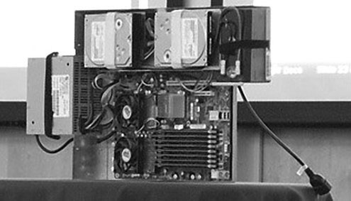
Figure 6.21 Server for Google WSC. The power supply is on the left and the two disks are on the top. The two fans below the left disk cover the two sockets of the AMD Barcelona microprocessor, each with two cores, running at 2.2 GHz. The eight DIMMs in the lower right each hold 1 GB, giving a total of 8 GB. There is no extra sheet metal, as the servers are plugged into the battery and a separate plenum is in the rack for each server to help control the airflow. In part because of the height of the batteries, 20 servers fit in a rack.

Google engineers realized that 12 volts meant that the UPS could simply be a standard battery on each shelf. Hence, rather than have a separate battery room, which Figure 6.9 shows as 94% efficient, each server has its own lead acid battery that is 99.99% efficient. This “distributed UPS” is deployed incrementally with each machine, which means there is no money or power spent on overcapacity. They use standard off-the-shelf UPS units to protect network switches.

What about saving power by using dynamic voltage-frequency scaling (DVFS), which Chapter 1 describes? DVFS was not deployed in this family of machines since the impact on latency was such that it was only feasible in very low activity regions for online workloads, and even in those cases the system-wide savings were very small. The complex management control loop needed to deploy it therefore could not be justified.

One of the keys to achieving the PUE of 1.23 was to put measurement devices (called current transformers) in all circuits throughout the containers and elsewhere in the WSC to measure the actual power usage. These measurements allowed Google to tune the design of the WSC over time.

Google publishes the PUE of its WSCs each quarter. Figure 6.22 plots the PUE for 10 Google WSCs from the third quarter in 2007 to the second quarter in 2010; this section describes the WSC labeled Google A. Google E operates with a PUE of 1.16 with cooling being only 0.105, due to the higher operational temperatures and chiller cutouts. Power distribution is just 0.039, due to the distributed UPS and single voltage power supply. The best WSC result was 1.12, with Google A at 1.23. In April 2009, the trailing 12-month average weighted by usage across all datacenters was 1.19.

Figure 6.22 Power usage effectiveness (PUE) of 10 Google WSCs over time. Google A is the WSC described in this section. It is the highest line in Q3 ’07 and Q2 ’10. (From www.google.com/corporate/green/datacenters/measuring.htm.) Facebook recently announced a new datacenter that should deliver an impressive PUE of 1.07 (see http://opencompute.org/). The Prineville Oregon Facility has no air conditioning and no chilled water. It relies strictly on outside air, which is brought in one side of the building, filtered, cooled via misters, pumped across the IT equipment, and then sent out the building by exhaust fans. In addition, the servers use a custom power supply that allows the power distribution system to skip one of the voltage conversion steps in Figure 6.9.

Servers in a Google WSC

The server in Figure 6.21 has two sockets, each containing a dual-core AMD Opteron processor running at 2.2 GHz. The photo shows eight DIMMS, and these servers are typically deployed with 8 GB of DDR2 DRAM. A novel feature is that the memory bus is downclocked to 533 MHz from the standard 666 MHz since the slower bus has little impact on performance but a significant impact on power.

The baseline design has a single network interface card (NIC) for a 1 Gbit/sec Ethernet link. Although the photo in Figure 6.21 shows two SATA disk drives, the baseline server has just one. The peak power of the baseline is about 160 watts, and idle power is 85 watts.

This baseline node is supplemented to offer a storage (or “diskfull”) node. First, a second tray containing 10 SATA disks is connected to the server. To get one more disk, a second disk is placed into the empty spot on the motherboard, giving the storage node 12 SATA disks. Finally, since a storage node could saturate a single 1 Gbit/sec Ethernet link, a second Ethernet NIC was added. Peak power for a storage node is about 300 watts, and it idles at 198 watts.

Note that the storage node takes up two slots in the rack, which is one reason why Google deployed 40,000 instead of 52,200 servers in the 45 containers. In this facility, the ratio was about two compute nodes for every storage node, but that ratio varied widely across Google’s WSCs. Hence, Google A had about 190,000 disks in 2007, or an average of almost 5 disks per server.

Networking in a Google WSC

The 40,000 servers are divided into three arrays of more than 10,000 servers each. (Arrays are called clusters in Google terminology.) The 48-port rack switch uses 40 ports to connect to servers, leaving 8 for uplinks to the array switches.

Array switches are configured to support up to 480 1 Gbit/sec Ethernet links and a few 10 Gbit/sec ports. The 1 Gigabit ports are used to connect to the rack switches, as each rack switch has a single link to each of the array switches. The 10 Gbit/sec ports connect to each of two datacenter routers, which aggregate all array routers and provide connectivity to the outside world. The WSC uses two datacenter routers for dependability, so a single datacenter router failure does not take out the whole WSC.

The number of uplink ports used per rack switch varies from a minimum of 2 to a maximum of 8. In the dual-port case, rack switches operate at an oversubscription rate of 20:1. That is, there is 20 times the network bandwidth inside the switch as there was exiting the switch. Applications with significant traffic demands beyond a rack tended to suffer from poor network performance. Hence, the 8-port uplink design, which provided a lower oversubscription rate of just 5:1, was used for arrays with more demanding traffic requirements.

Monitoring and Repair in a Google WSC

For a single operator to be responsible for more than 1000 servers, you need an extensive monitoring infrastructure and some automation to help with routine events.

Google deploys monitoring software to track the health of all servers and networking gear. Diagnostics are running all the time. When a system fails, many of the possible problems have simple automated solutions. In this case, the next step is to reboot the system and then to try to reinstall software components. Thus, the procedure handles the majority of the failures.

Machines that fail these first steps are added to a queue of machines to be repaired. The diagnosis of the problem is placed into the queue along with the ID of the failed machine.

To amortize the cost of repair, failed machines are addressed in batches by repair technicians. When the diagnosis software is confident in its assessment, the part is immediately replaced without going through the manual diagnosis process. For example, if the diagnostic says disk 3 of a storage node is bad, the disk is replaced immediately. Failed machines with no diagnostic or with low-confidence diagnostics are examined manually.

The goal is to have less than 1% of all nodes in the manual repair queue at any one time. The average time in the repair queue is a week, even though it takes much less time for repair technician to fix it. The longer latency suggests the importance of repair throughput, which affects cost of operations. Note that the automated repairs of the first step take minutes for a reboot/reinstall to hours for running directed stress tests to make sure the machine is indeed operational.

These latencies do not take into account the time to idle the broken servers. The reason is that a big variable is the amount of state in the node. A stateless node takes much less time than a storage node whose data may need to be evacuated before it can be replaced.

Summary

As of 2007, Google had already demonstrated several innovations to improve the energy efficiency of its WSCs to deliver a PUE of 1.23 in Google A:

In addition to providing an inexpensive shell to enclose servers, the modified shipping containers separate hot and cold air plenums, which helps reduce the variation in intake air temperature for servers. With less severe worst-case hot spots, cold air can be delivered at warmer temperatures.

These containers also shrink the distance of the air circulation loop, which reduces energy to move air.

Operating servers at higher temperatures means that air only has to be chilled to 81°F (27°C) instead of the traditional 64°F to 71°F (18°C to 22°C).

A higher target cold air temperature helps put the facility more often within the range that can be sustained by evaporative cooling solutions (cooling towers), which are more energy efficient than traditional chillers.

Deploying WSCs in temperate climates to allow use of evaporative cooling exclusively for portions of the year.

Deploying extensive monitoring hardware and software to measure actual PUE versus designed PUE improves operational efficiency.

Operating more servers than the worst-case scenario for the power distribution system would suggest, since it’s statistically unlikely that thousands of servers would all be highly busy simultaneously, yet rely on the monitoring system to off-load work in the unlikely case that they did [Fan, Weber, and Barroso 2007] [Ranganathan et al. 2006]. PUE improves because the facility is operating closer to its fully designed capacity, where it is at its most efficient because the servers and cooling systems are not energy proportional. Such increased utilization reduces demand for new servers and new WSCs.

Designing motherboards that only need a single 12-volt supply so that the UPS function could be supplied by standard batteries associated with each server instead of a battery room, thereby lowering costs and reducing one source of inefficiency of power distribution within a WSC.

Carefully designing the server board itself to improve its energy efficiency. For example, underclocking the front-side bus on these microprocessors reduces energy usage with negligible performance impact. (Note that such optimizations do not impact PUE but do reduce overall WSC energy consumption.)

WSC design must have improved in the intervening years, as Google’s best WSC has dropped the PUE from 1.23 for Google A to 1.12. Facebook announced in 2011 that they had driven PUE down to 1.07 in their new datacenter (see http://opencompute.org/). It will be interesting to see what innovations remain to improve further the WSC efficiency so that we are good guardians of our environment. Perhaps in the future we will even consider the energy cost to manufacture the equipment within a WSC [Chang et al. 2010].

Case Study 1: Total Cost of Ownership Influencing Warehouse-Scale Computer Design Decisions

Concepts illustrated by this case study

Total Cost of Ownership (TCO)

Influence of Server Cost and Power on the Entire WSC

Benefits and Drawbacks of Low-Power Servers

Total cost of ownership is an important metric for measuring the effectiveness of a warehouse-scale computer (WSC). TCO includes both the CAPEX and OPEX described in Section 6.4 and reflects the ownership cost of the entire datacenter to achieve a certain level of performance. In considering different servers, networks, and storage architectures, TCO is often the important comparison metric used by datacenter owners to decide which options are best; however, TCO is a multidimensional computation that takes into account many different factors. The goal of this case study is to take a detailed look into WSCs, how different architectures influence TCO, and how TCO drives operator decisions. This case study will use the numbers from Figure 6.13 and Section 6.4, and assumes that the described WSC achieves the operator’s target level of performance. TCO is often used to compare different server options that have multiple dimensions. The exercises in this case study examine how such comparisons are made in the context of WSCs and the complexity involved in making the decisions.

6.1 [5/5/10] <6.2, 6.4> In this chapter, data-level parallelism has been discussed as a way for WSCs to achieve high performance on large problems. Conceivably, even greater performance can be obtained by using high-end servers; however, higher performance servers often come with a nonlinear price increase.

a. [5] <6.4> Assuming servers that are 10% faster at the same utilization, but 20% more expensive, what is the CAPEX for the WSC?

b. [5] <6.4> If those servers also use 15% more power, what is the OPEX?

c. [10] <6.2, 6.4> Given the speed improvement and power increase, what must the cost of the new servers be to be comparable to the original cluster? (Hint: Based on this TCO model, you may have to change the critical load of the facility.)

6.2 [5/10] <6.4, 6.8> To achieve a lower OPEX, one appealing alternative is to use low-power versions of servers to reduce the total electricity required to run the servers; however, similar to high-end servers, low-power versions of high-end components also have nonlinear trade-offs.

a. [5] <6.4, 6.8> If low-power server options offered 15% lower power at the same performance but are 20% more expensive, are they a good trade-off?

b. [10] <6.4, 6.8> At what cost do the servers become comparable to the original cluster? What if the price of electricity doubles?

6.3 [5/10/15] <6.4, 6.6> Servers that have different operating modes offer opportunities for dynamically running different configurations in the cluster to match workload usage. Use the data in Figure 6.23 for the power/performance modes for a given low-power server.

Figure 6.23 Power–performance modes for low-power servers.

a. [5] <6.4, 6.6> If a server operator decided to save power costs by running all servers at medium performance, how many servers would be needed to achieve the same level of performance?

b. [10] <6.4, 6.6> What are the CAPEX and OPEX of such a configuration?

c. [15] <6.4, 6.6> If there was an alternative to purchase a server that is 20% cheaper but slower and uses less power, find the performance–power curve that provides a TCO comparable to the baseline server.

6.4 [Discussion] <6.4> Discuss the trade-offs and benefits of the two options in Exercise 6.3, assuming a constant workload being run on the servers.

6.5 [Discussion] <6.2, 6.4> Unlike high-performance computing (HPC) clusters, WSCs often experience significant workload fluctuation throughout the day. Discuss the trade-offs and benefits of the two options in Exercise 6.3, this time assuming a workload that varies.

6.6 [Discussion] <6.4, 6.7> The TCO model presented so far abstracts away a significant amount of lower level details. Discuss the impact of these abstractions to the overall accuracy of the TCO model. When are these abstractions safe to make? In what cases would greater detail provide significantly different answers?

Case Study 2: Resource Allocation in WSCs and TCO

Concepts illustrated by this case study

Server and Power Provisioning within a WSC

Time-Variance of Workloads

Effects of Variance on TCO

Some of the key challenges to deploying efficient WSCs are provisioning resources properly and utilizing them to their fullest. This problem is complex due to the size of WSCs as well as the potential variance of the workloads being run. The exercises in this case study show how different uses of resources can affect TCO.

6.7 [5/5/10] <6.4> One of the challenges in provisioning a WSC is determining the proper power load, given the facility size. As described in the chapter, nameplate power is often a peak value that is rarely encountered.

a. [5] <6.4> Estimate how the per-server TCO changes if the nameplate server power is 200 watts and the cost is $3000.

b. [5] <6.4> Also consider a higher power, but cheaper option whose power is 300 watts and costs $2000.

c. [10] <6.4> How does the per-server TCO change if the actual average power usage of the servers is only 70% of the nameplate power?

6.8 [15/10] <6.2, 6.4> One assumption in the TCO model is that the critical load of the facility is fixed, and the amount of servers fits that critical load. In reality, due to the variations of server power based on load, the critical power used by a facility can vary at any given time. Operators must initially provision the datacenter based on its critical power resources and an estimate of how much power is used by the datacenter components.

a. [15] <6.2, 6.4> Extend the TCO model to initially provision a WSC based on a server with a nameplate power of 300 watts, but also calculate the actual monthly critical power used and TCO assuming the server averages 40% utilization and 225 watts. How much capacity is left unused?

b. [10] <6.2, 6.4> Repeat this exercise with a 500-watt server that averages 20% utilization and 300 watts.

6.9 [10] <6.4, 6.5> WSCs are often used in an interactive manner with end users, as mentioned in Section 6.5. This interactive usage often leads to time-of-day fluctuations, with peaks correlating to specific time periods. For example, for Netflix rentals, there is a peak during the evening periods of 8 to 10 p.m.; the entirety of these time-of-day effects is significant. Compare the per-server TCO of a datacenter with a capacity to match the utilization at 4 a.m. compared to 9 p.m.

6.10 [Discussion/15] <6.4, 6.5> Discuss some options to better utilize the excess servers during the off-peak hours or options to save costs. Given the interactive nature of WSCs, what are some of the challenges to aggressively reducing power usage?

6.11 [Discussion/25] <6.4, 6.6> Propose one possible way to improve TCO by focusing on reducing server power. What are the challenges to evaluating your proposal? Estimate the TCO improvements based on your proposal. What are advantages and drawbacks?

Exercises

6.16 [15/15/20/15/] <6.1, 6.2, 6.8> Although request-level parallelism allows many machines to work on a single problem in parallel, thereby achieving greater overall performance, one of the challenges is avoiding dividing the problem too finely. If we look at this problem in the context of service level agreements (SLAs), using smaller problem sizes through greater partitioning can require increased effort to achieve the target SLA. Assume an SLA of 95% of queries respond at 0.5 sec or faster, and a parallel architecture similar to MapReduce that can launch multiple redundant jobs to achieve the same result. For the following questions, assume the query–response time curve shown in Figure 6.24. The curve shows the latency of response, based on the number of queries per second, for a baseline server as well as a “small” server that uses a slower processor model.

Figure 6.24 Query–response time curve.

a. [15] <6.1, 6.2, 6.8> How many servers are required to achieve that SLA, assuming that the WSC receives 30,000 queries per second, and the query–response time curve shown in Figure 6.24? How many “small” servers are required to achieve that SLA, given this response-time probability curve? Looking only at server costs, how much cheaper must the “wimpy” servers be than the normal servers to achieve a cost advantage for the target SLA?

b. [15] <6.1, 6.2, 6.8> Often “small” servers are also less reliable due to cheaper components. Using the numbers from Figure 6.1, assume that the number of events due to flaky machines and bad memories increases by 30%. How many “small” servers are required now? How much cheaper must those servers be than the standard servers?

c. [20] <6.1, 6.2, 6.8> Now assume a batch processing environment. The “small” servers provide 30% of the overall performance of the regular servers. Still assuming the reliability numbers from Exercise 6.15 part (b), how many “wimpy” nodes are required to provide the same expected throughput of a 2400-node array of standard servers, assuming perfect linear scaling of performance to node size and an average task length of 10 minutes per node? What if the scaling is 85%? 60%?

d. [15] <6.1, 6.2, 6.8> Often the scaling is not a linear function, but instead a logarithmic function. A natural response may be instead to purchase larger nodes that have more computational power per node to minimize the array size. Discuss some of the trade-offs with this architecture.

6.25 [5/Discussion/10/15/Discussion/Discussion/Discussion] <6.4> Power stranding is a term used to refer to power capacity that is provisioned but not used in a datacenter. Consider the data presented in Figure 6.25 [Fan, Weber, and Barroso 2007] for different groups of machines. (Note that what this paper calls a “cluster” is what we have referred to as an “array” in this chapter.)

Figure 6.25 Cumulative distribution function (CDF) of a real datacenter.

a. [5] What is the stranded power at (1) the rack level, (2) the power distribution unit level, and (3) the array (cluster) level? What are the trends with oversubscription of power capacity at larger groups of machines?

b. [Discussion] What do you think causes the differences between power stranding at different groups of machines?

c. [10] Consider an array-level collection of machines where the total machines never use more than 72% of the aggregate power (this is sometimes also referred to as the ratio between the peak-of-sum and sum-of-peaks usage). Using the cost model in the case study, compute the cost savings from comparing a datacenter provisioned for peak capacity and one provisioned for actual use.

d. [15] Assume that the datacenter designer chose to include additional servers at the array level to take advantage of the stranded power. Using the example configuration and assumptions in part (a), compute how many more servers can now be included in the warehouse-scale computer for the same total power provisioning.

e. [Discussion] What is needed to make the optimization of part (d) work in a real-world deployment? (Hint: Think about what needs to happen to cap power in the rare case when all the servers in the array are used at peak power.)

f. [Discussion] Two kinds of policies can be envisioned to manage power caps [Ranganathan et al. 2006]: (1) preemptive policies where power budgets are predetermined (“don’t assume you can use more power; ask before you do!”) or (2) reactive policies where power budgets are throttled in the event of a power budget violation (“use as much power as needed until told you can’t!”). Discuss the trade-offs between these approaches and when you would use each type.

g. [Discussion] What happens to the total stranded power if systems become more energy proportional (assume workloads similar to that of Figure 6.4)?

6.30 [15/20/20] <6.2, 6.6> This exercise illustrates the interactions of energy proportionality models with optimizations such as server consolidation and energy-efficient server designs. Consider the scenarios shown in Figure 6.26 and Figure 6.27.

Figure 6.26 Power distribution for two servers.

Figure 6.27 Utilization distributions across cluster, without and with consolidation.

a. [15] Consider two servers with the power distributions shown in Figure 6.26: case A (the server considered in Figure 6.4) and case B (a less energy-proportional but more energy-efficient server than case A). Assume the system utilization mix in column 7 of Figure 6.4. For simplicity, assume a discrete distribution across 1000 servers, with 109 servers at 0% utilization, 80 servers at 10% utilizations, etc., as shown in row 1 of Figure 6.27. Assume performance variation based on column 2 of Figure 6.4. Compare the total performance and total energy for this workload mix for the two server types.

b. [20] Consider a cluster of 1000 servers with data similar to the data shown in Figure 6.4 (and summarized in the first rows of Figures 6.26 and 6.27). What are the total performance and total energy for the workload mix with these assumptions? Now assume that we were able to consolidate the workloads to model the distribution shown in case C (second row of Figure 6.27). What are the total performance and total energy now? How does the total energy compare with a system that has a linear energy-proportional model with idle power of zero watts and peak power of 662 watts?

c. [20] Repeat part (b), but with the power model of server B, and compare with the results of part (a).

6.31 [10/Discussion] <6.2, 6.4, 6.6> System-Level Energy Proportionality Trends: Consider the following breakdowns of the power consumption of a server:

CPU, 50%; memory, 23%; disks, 11%; networking/other, 16%

CPU, 33%; memory, 30%; disks, 10%; networking/other, 27%

a. [10] Assume a dynamic power range of 3.0× for the CPU (i.e., the power consumption of the CPU at idle is one-third that of its power consumption at peak). Assume that the dynamic range of the memory systems, disks, and the networking/other categories above are respectively 2.0×, 1.3×, and 1.2×. What is the overall dynamic range for the total system for the two cases?

Figure 6.28 Overview of data center tier classifications. (Adapted from Pitt Turner IV et al. [2008].)

b. [Discussion/10] What can you learn from the results of part (a)? How would we achieve better energy proportionality at the system level? (Hint: Energy proportionality at a system level cannot be achieved through CPU optimizations alone, but instead requires improvement across all components.)