Chapter 6

Solar-Cell-Integrated Antennas

6.1 Integration of Antennas with Solar Cells

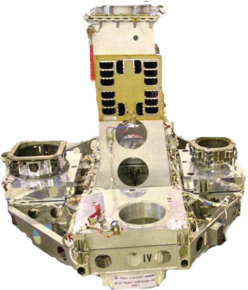
A solar cell is also known as a photovoltaic or photoelectric cell. It is a device that converts sunlight into electricity. The photovoltaic effect was found by a French physicist, A. E. Becquerel, in 1839, and the phenomenon was later explained by A. Einstein, in 1905. Materials used for modern photovoltaic cells include monocrystalline and polycrystalline silicon, amorphous silicon, cadmium telluride, copper indium selenide/sulfide, and many others. In the past two decades, some work has been reported on the integration of different antennas with solar cell panels (1, 10). Most solar-cell-integrated antennas were used for space-related applications. Figure 6.1 is a photograph showing a satellite bearing antennas and solar cells on different parts of its body. As can be seen from the figure, the two components usually constitute a large surface area. This is very undesirable, as size and weight are among the scarcest resources on a satellite! In 1995, Tanaka et al. (1) covered the resonator and ground surfaces of a microstrip patch antenna with photovoltaic panels. The solar-cell-loaded microstrip antennas were then used in designing a microsatellite. Later, Vaccaro et al. (2, 3) proposed etching slot antennas on a solar cell panel, at the expense of reducing the effective illumination area. The configuration of Vaccaro's solar-cell-loaded antenna, which is called Solant, is shown in Fig. 6.2. By cascading six antennas into a 1 × 6 array, it was demonstrated that solar cells were able to supply a power of 0.821 W with 122 mA at 7 V. An antenna gain of 10 to 11 dBi was also obtained. Shown in Fig 6.3 is the proposed Solant, which was tested for an in-flight space mission (4).

Figure 6.1 Antennas and solar cell panels of a satellite.

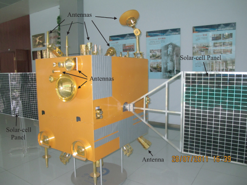
Figure 6.2 Configuration of the Solant. (Courtesy of S. Vaccaro, JAST Antenna Systems, Switzerland. From (2), copyright © 2003 IEEE, with permission.)

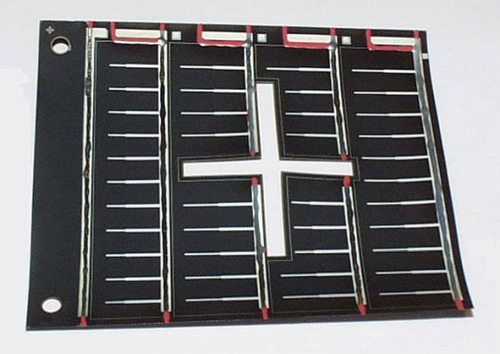
Figure 6.3 Solants placed on a satellite. (Courtesy of S. Vaccaro, JAST Antenna Systems, Switzerland. From (4), copyright © 2009 IEEE, with permission.)

As solar-cell-integrated antennas are generally used for outer-space missions, they are required to satisfy the following stringent requirements:

There are two ways to design solar-cell-integrated antennas. The first is to make use of the solar cell itself as an antenna. As reported by Vaccaro et al. (6), with the simultaneous use of a GaAs solar cell panel itself as an electromagnetic radiator, the antenna gain of the solar-cell-integrated antenna was found to be about 10 dB lower than for the microstrip patch antenna made of copper. Ons et al. (14) suspended a semiconductor-made dipole, itself also a solar cell, at the focus of a solar concentrator designed for collecting solar energy. For the second approach, the antenna and solar cell are made separately but closely integrated into a single module (7). An effort is required to minimize the interference between the two components. For both methods, however, the antenna gains of the solar-cell-integrated antennas are usually lower than those for their isolated counterparts, probably due to the semiconductor and dielectric losses of the solar cell materials. Some other design issues also need to be looked into. Hwu et al. (8) found that solar cell panels could scatter electromagnetic fields and cause the antenna gain to degrade. Tomisawa and Toruda (9) showed that an antenna could cause a neighboring solar cell to radiate ambient signals, introducing additional noise to the wireless system.

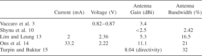
Many solar-cell-integrated antennas have been reported in the past few decades, with some of the performances highlighted in Table 6.1. In some studies (2–6), part of the solar cell panel was removed to construct a slot antenna. For other design approaches (10–12), a metallic antenna is designed independently and placed directly on top of a solar cell panel, which also functions as the ground plane of the antenna. In this case, however, the antenna substrate partially blocks the solar cell panel from sunlight reception. To solve this problem, a transparent DRA has been stacked directly on top of a solar cell (13). Here, the DRA functions simultaneously as a radiating element as well as a focusing lens. Turpin and Baktur (15) integrated meshed patch antennas on solar cell panels for the design of a diversity antenna.

Table 6.1 Performance Reported for Solar-Cell-Integrated Antennas

It is always desirable to maximize the surface area of the solar cell so that larger electrical output can be obtained. On the other hand, use of a large number of solar cell panels should be avoided, as it can affect antenna performance. Designing a solar-cell-integrated antenna is sometimes a compromise between the two.

6.2 Nonplanar Solar-cell-integrated Antennas

Here, the integration of the dielectric resonator antenna (DRA) and solar cell is explored. In the past two decades, the DRA has been studied extensively because of its small size, low loss, low cost, light weight, and ease of excitation (16, 17). With the use of DR, the antenna size can be usually scaled down by a factor of , where ε _r is the dielectric constant of the DR. This feature is very useful for reducing the antenna size. In modern wireless gadgets, compactness is always one of the topmost priorities (18). This necessitates the development of multifunction components to miniaturize the system.

6.2.1 Solar-Cell-Integrated Hemispherical DRA

It is well known that a lens is a very important component for optical systems. Therefore, it has been of great interest to develop a dual-functional antenna that additionally provides the function of a lens. A dual-functional transparent hemispherical DRA that simultaneously functions as an antenna and a focusing lens for a solar cell was investigated for the first time by Lim and Leung (13). To make the entire system even more compact, the solar cell is placed beneath the DRA to save the footprint. Here, it is worth mentioning that the DRA can also serve as a protective cover for the solar cell. A conformal strip is used to excite the transparent hemispherical DRA in its dominant mode, TE₁₁₁. It was found that due to its focusing effect, the transparent hemispherical DR can be used to increase the output voltage and current of the solar-cell-integrated DRA.

6.2.1.1 Configuration

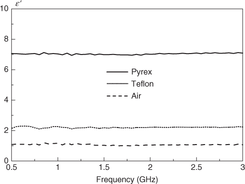
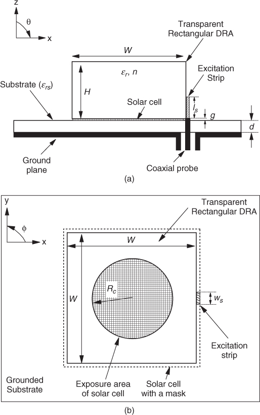
Figure 6.4 shows the configuration of a dual-functional hemispherical DRA. The transparent DRA (19) was made of borosilicate crown glass, which is commonly known as K9 glass or Pyrex. It has a radius of R = 28 mm and is placed above the solar cell. A conformal strip with a width of w_s = 12 mm and a length of l_s = 19 mm was used to feed the DRA, which was excited in its fundamental mode at 1.87 GHz. The design methods and equations are available in the literature (20–23). By using an Agilent 85070D dielectric probe kit, the dielectric constant of the glass was measured (Fig. 6.5). It was found that the dielectric constant of Pyrex is ε _r ∼ 7 in the frequency range 0.5 to 3 GHz. For verification purposes, the dielectric constants of two well-known materials, air and Teflon, were measured using the same calibrated probe. It was found that the probe was well calibrated, as the measured values were very close to those given by specifications (air, ε _r ∼ 1, and Teflon, ε _r ∼ 2.2). For all subsequent simulations, the dielectric constant is taken to be ε _r ∼ 7 around 1.9 GHz. At optical frequencies, the glass has a much lower dielectric constant of ε _r ∼ 2.17, which was calculated from its refractive index of n = 1.474 (19, 24).

Figure 6.4 Dual-functional transparent hemispherical DRA with an underlaid solar cell: (a) front view; (b) top view. (From (13), copyright © 2010 IEEE, with permission.)

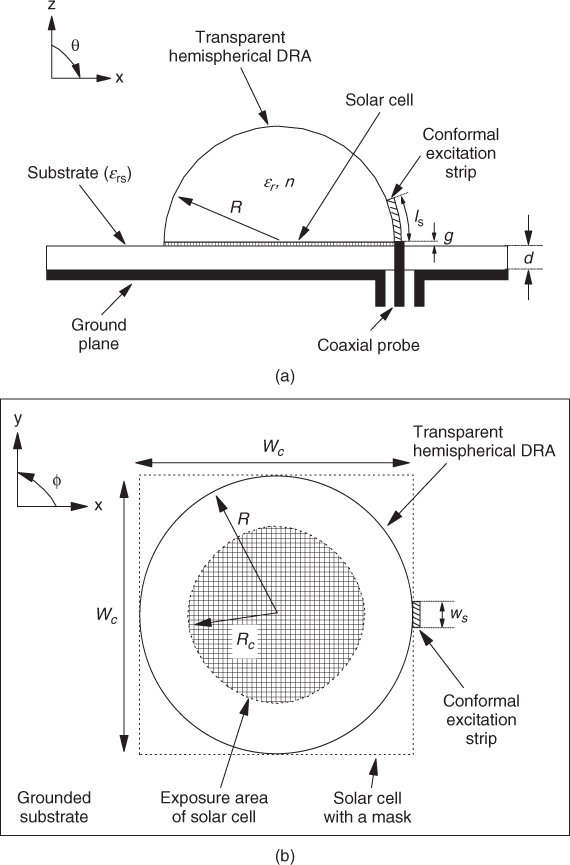
Figure 6.5 Dielectric constants measured for Pyrex, air, and Teflon.

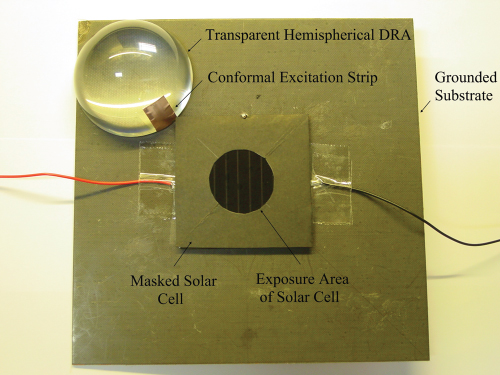
A square solar cell was used to construct the solar-cell-integrated DRA in Fig. 6.4. But since the dielectric properties of the solar cell were not available, the values of ε _r = 1.5 and tan δ = 10 reported for a solar cell (25) were used in our HFSS simulations. With reference to the figure, the solar cell panel has a side length of W_c = 55 mm and a thickness of 1.8 mm. The left and right output pins (for output connection) at the back of the solar cell panel have a height of 0.2 mm. Because of the thickness of the solar cell (1.8 mm) and the height of the output pins (0.2 mm), the DRA has a displacement of 2 mm from the substrate. This information was also used in our HFSS simulations. The substrate has a dielectric constant of ε _rs = 2.33, a thickness of d = 1.57 mm, and a size of 16 × 16 cm². It serves as an additional insulator between the solar cell and the ground plane. In the experiment, the output pins of the solar cell were connected to a voltmeter and an ammeter for measurements of the voltage and current, respectively. To study the focusing effect of the DRA, the square solar cell is masked with a circular exposure area of radius R_c. A very thin, dark, hard paper was used as the mask and not included in the simulations. Figure 6.6 shows the prototype.

Figure 6.6 Transparent hemispherical DRA and solar cell panel. The wires are for the power output of the solar-cell panel. In the actual configuration, the transparent hemispherical DRA is placed on top of the panel. (From (13), copyright © 2010 IEEE, with permission.)

6.2.1.2 Antenna Performances: Results and Discussion

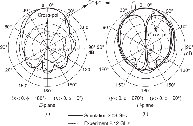
Ansoft HFSS was used to simulate the antenna part of a solar-cell-integrated DRA, and measurements were carried out using the Agilent 8753 to verify the results. Without considering the solar cell, the effect of the airgap between the DRA and the substrate is studied first. Figure 6.7 shows the reflection coefficients of the DRA measured and simulated for g = 0 and 2 mm, where reasonable agreement between the results is observed for each case. With reference to the figure, the airgap causes the resonance frequency and impedance bandwidth measured (|S₁₁| ≤ − 10 dB) to increase from 1.92 GHz to 2.26 GHz and from 14% to 19%, respectively. The trends are expected because similar results were obtained for the cylindrical and ring DRAs reported in the literature (26–28). The input impedances simulated and measured for g = 0 and 2 mm are shown in Fig. 6.8. As can be seen from the figure, the airgap causes the antenna to be more inductive. The antenna gains of the two DRAs (g = 0 and 2 mm) were also measured. As can be seen in Fig. 6.9, they are in the range 4 to 6.8 dBi across their passbands. It is found that the antenna gain is maximum around the resonance for each case, which is typical for the DRA. The radiation patterns for g = 0 mm are shown in Fig. 6.10. As can be observed from the figure, the co-polarized fields of both the E- and H-planes are stronger than the cross-polarized fields by more than 20 dB in the bore-sight direction (θ = 0°). Similar results were observed for g = 2 mm in Fig. 6.11.

Figure 6.7 Reflection coefficients of hemispherical DRAs simulated and measured for g = 0 and 2 mm. The results were obtained with no underlaid solar cell. (From (13), copyright © 2010 IEEE, with permission.)

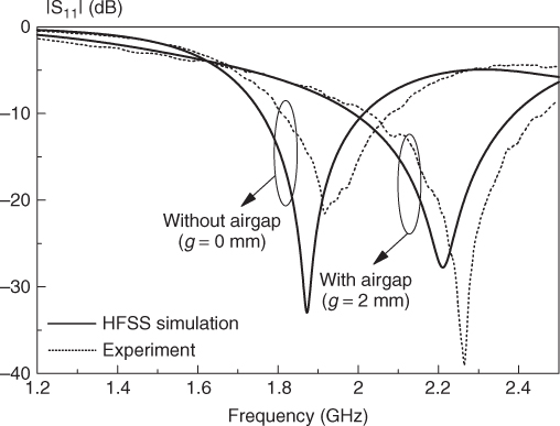
Figure 6.8 Input impedances simulated and measured for hemispherical DRAs for (a) g = 0 and (b) 2 mm. The results were obtained with no underlaid solar cell.

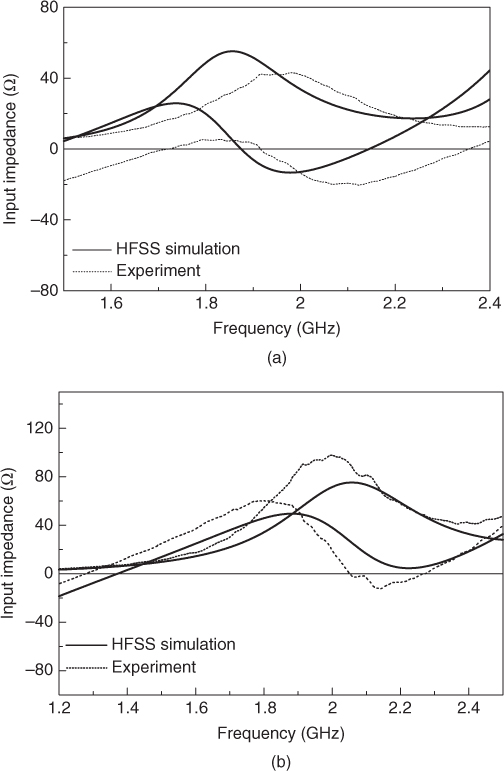
Figure 6.9 Antennas gains of hemispherical DRAs measured for g = 0 and 2 mm. The results were obtained with no underlaid solar cell. (From (13), copyright © 2010 IEEE, with permission.)

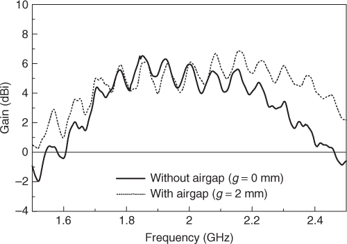
Figure 6.10 Normalized radiation patterns of a hemispherical DRA simulated and measured for g = 0 mm. There is no underlaid solar cell. (a) E-plane; (b) H-plane. (From (13), copyright © 2010 IEEE, with permission.)

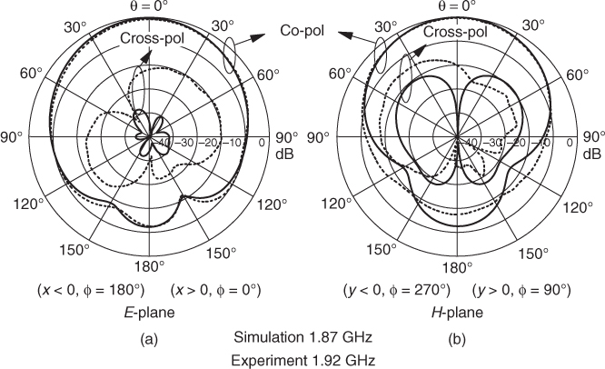
Figure 6.11 Normalized radiation patterns of a hemispherical DRA simulated and measured for g = 2 mm. There is no underlaid solar cell. (a) E-plane; (b) H-plane. (From (13), copyright © 2010 IEEE, with permission.)

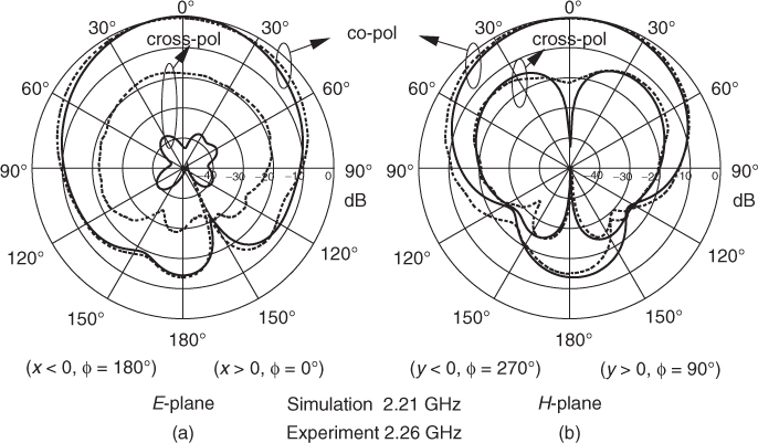
Next, the characteristics of the DRA with the underlaid solar cell (Fig. 6.4) are investigated. Figure 6.12 shows the reflection coefficients simulated and measured for the configuration. As can be observed from the figure, the resonance frequencies of the DRA measured and simulated are 1.94 and 1.89 GHz, respectively, with an error of 2.65%. The impedance bandwidths measured and simulated are given by 16.5% and 22.8%, respectively. Although the DRA in this case also has a displacement of 2 mm from the substrate as for the previous one with the airgap, its measured resonance frequency (1.94 GHz) is lower than that of the airgap case (2.26 GHz). This is because the solar cell increases the effective dielectric constant of the system. It is interesting to note that the resonance frequency measured (1.94 GHz) is quite close to that of the previous DRA (1.92 GHz) resting on the ground plane (g = 0 mm). With reference to the figure, a small resonance mode was measured at 2.25 GHz. This mode is caused by the solar cell, which can be verified by the fact that it was still observed when a rectangular DRA was used (this will be shown later). The result simulated does not predict this resonance mode, which is not surprising because the exact dielectric parameters of the solar cell are not known.

Figure 6.12 Reflection coefficients simulated and measured for a hemispherical DRA with an underlaid solar cell (Fig. 6.4). Their corresponding input impedances are shown in the inset. (From (13), copyright © 2010 IEEE, with permission.)

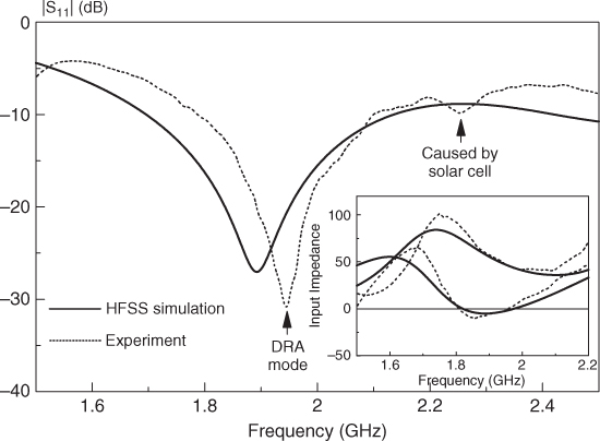
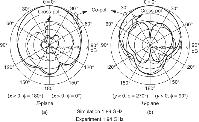
Figure 6.13 shows the antenna gains of the DRA measured with and without the underlaid solar cell. With reference to the figure, the two antenna gains are very close to each other around the resonance of the DRA. This is a very positive result, as it implies that the loss due to the solar cell is negligibly small. It is observed from the figure that the gain is about 5.3 dBi around the resonance. Figure 6.14 shows the E- and H-plane radiation patterns measured and simulated. As can be

seen from the figure, the co-polarized fields are stronger than their cross-polarized counterparts by at least 22 dB in the bore-sight direction.

Figure 6.13 Antenna gains measured for a hemispherical DRA with and without (g = 0 mm) a solar cell. (From (13), copyright © 2010 IEEE, with permission.)

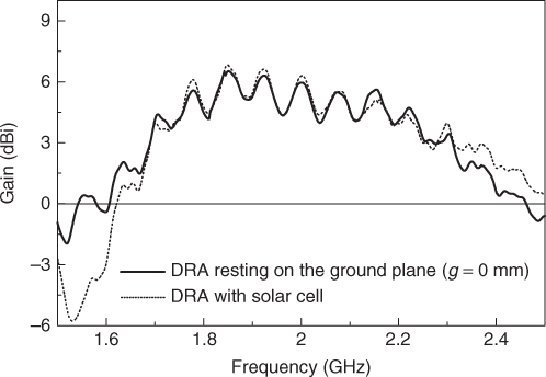
Figure 6.14 Normalized radiation patterns simulated and measured for a hemispherical DRA with an underlaid solar cell. (a) E-planel (b) H-plane. (From (13), copyright © 2010 IEEE, with permission.)

6.2.1.3 Optical Performances: Results and Discussion

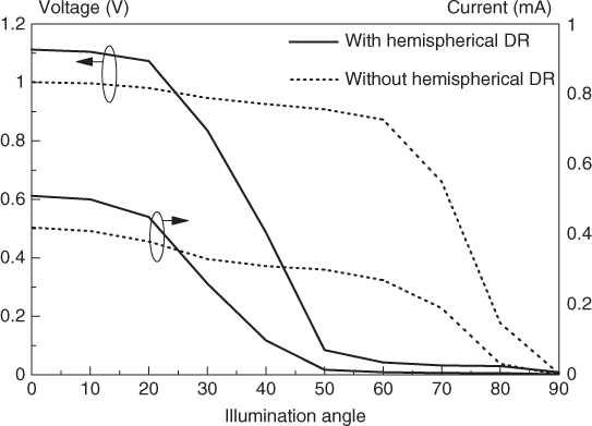
As can be seen in Fig. 6.15, a hemispherical lens itself is a good focusing lens for light. The length of the focus can be obtained by f_i = Rn₂/(n₂ − n₁), where R is the center of the sphere, and n₁ and n₂ are reflective indexes of the two light-guiding materials (29). In this case, n₁ is for air and n₂ is for Pyrex. The optical performance of the solar-cell-integrated DRA in Fig. 6.4 is now evaluated. A coherent Sabre Innova argon laser was used in the optical measurements. Parallel blue light beams at a wavelength of 488 nm were generated. The laser was tuned and provided an even light power of 130 mW to the DRA. To measure the outputs of the solar cell at different illumination angles (θ), the DRA was placed on a rotator, as shown in Fig. 6.16. As can be seen from the figure, a convex lens is used for spreading laser point source into a parallel light beam which is large enough to cover the entire DRA. Figure 6.17 shows the output voltage and current of the solar cell measured as a function of the illumination angle for R_c = 15 mm. Also shown in the figure are the outputs without the DRA. With reference to the figure, larger outputs can be obtained for θ ≤ 30° by using the DRA because of its focusing effect. With the DRA, the output voltage and current are increased by 13.5% and 27.2% at θ = 0°, respectively. A smaller radius of R_c = 10 mm was also used for the mask, and the result is shown in Fig. 6.18. Again, larger outputs were obtained for θ ≤ 30° when the DRA is present. In this case, the voltage and current outputs are increased by 11% and 21.4%, respectively, at θ = 0° with the use of the DRA. Finally, the voltage and current outputs are measured for a mask with R_c = 5 mm and, as can be seen in Fig. 6.19, an increase in the voltage and current outputs of 11.2% and 21.4% is observed for θ ≤ 25°. Another observation that can be made from the figures is that a larger illumination area is required to produce higher electricity output. In practical applications, the solar cell panel can be associated with a mechanical rotator so that it can track the light source if needed. In this case, the DRA proposed can be designed into a phased array so that it can scan the electromagnetic beam as the solar cell panel rotates.

Figure 6.15 Focusing length for a hemispherical lens with refractive index n₂.

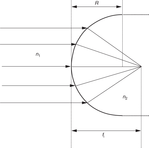
Figure 6.16 Top-down view of the coherent Sabre Innova argon laser system for generating a parallel blue light beam. (From (13), copyright © 2010 IEEE, with permission.)

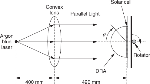
Figure 6.17 Output voltages and currents of a solar cell with and without the hemispherical DRA: R_c = 15 mm. (From (13), copyright © 2010 IEEE, with permission.)

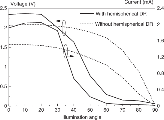
Figure 6.18 Output voltages and currents of a solar cell with and without the hemispherical DRA: R_c = 10 mm.

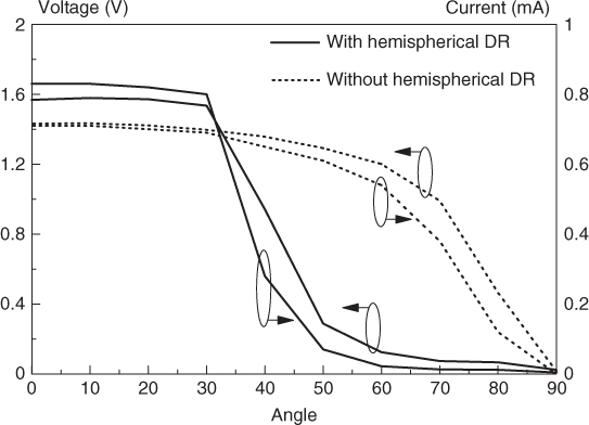
Figure 6.19 Output voltages and currents of a solar cell with and without the hemispherical DRA: R_c = 5 mm.

6.2.1.4 Antenna Array

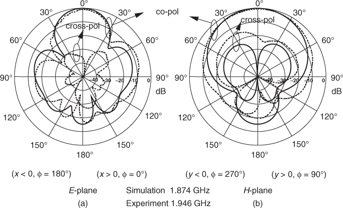
Two single-element DRAs (Fig. 6.4) are cascaded to form a 1 × 2 antenna array, shown in Fig. 6.20. A Krytar MLDD two-way in-phase power divider (Model 6005265 0.5 to 26.5 GHz) is used to feed the two DRAs. The reflection coefficient measured at the input port of the power divider (with the DRA array connected) is shown in Fig. 6.21. With reference to the figure, the DRA resonance frequency shifts to 1.98 GHz (as compared to 1.94 GHz for the single element). Other resonances at 1.85, 2.08, 2.28, and 2.43 GHz are inherent to the power divider. Next, the antenna gain measured for the DRA array is also given in Fig. 6.22. The maximum antenna gain reads about 8 dBi at 2 GHz. It is about 3 dB higher than the gain for the single-element DRA. Obviously, as can be seen in Fig. 6.23, the array effect is visible in the E-plane. A higher-order array can easily be obtained by cascading more DRA elements.

Figure 6.20 Top view of a dual-functional transparent hemispherical DRA array with underlaid solar cells.

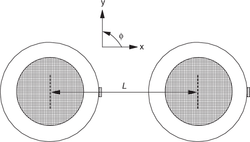
Figure 6.21 Reflection coefficient measured for a hemispherical DRA array with underlaid solar cells (Fig. 6.20).

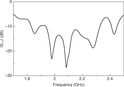
Figure 6.22 Antenna gain measured for a hemispherical DRA array with underlaid solar cells.

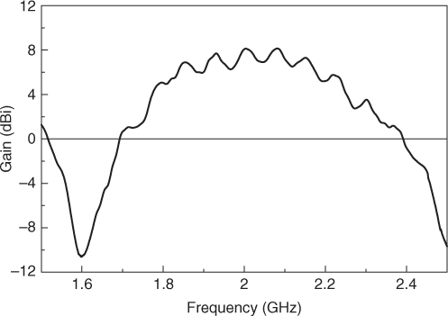
Figure 6.23 Normalized radiation patterns simulated and measured for a hemispherical DRA array with underlaid solar cells. (a) E-plane; (b) H-plane.

6.2.2 Solar-Cell-Integrated Rectangular DRA

6.2.2.1 Configuration

In this section the transparent rectangular DRA is also investigated for nonfocusing applications. For ease of comparison, the rectangular DRA was designed to resonate like the hemispherical DRA. The DRA was excited in its fundamental broadside TE₁₁₁ mode using a vertical excitation strip. Figure 6.24 shows a configuration with ε _r = 7, W = 50 mm, H = 22 mm, g = 2 mm, d = 1.57 mm, w_s = 12 mm, and l_s = 22 mm. The same masked solar cell was used again in this part.

Figure 6.24 Transparent rectangular DRA with an underlaid solar cell: (a) front view; (b) top view. (From (13), copyright © 2010 IEEE, with permission.)

6.2.2.2 Antenna Performances: Results and Discussion

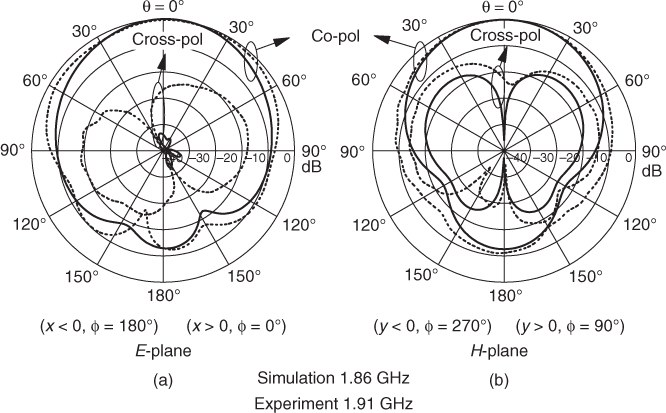
The antenna performances of the transparent rectangular solar-cell-integrated DRA are now discussed. Figure 6.25 shows the reflection coefficients that were simulated and measured, with their corresponding input impedances shown in the inset. As can be seen in the figure, the resonance frequencies of the DRA measured and simulated are given by 1.91 and 1.86 GHz, respectively, with an error of 2.7%. The impedance bandwidths measured and simulated are 17.6% and 15.8%, respectively. Again, the resonance due to the solar cell is observed in the measured result. Its resonance frequency shifts slightly from 2.25 GHz to 2.23 GHz due to the changes in the dielectric and excitation-strip loadings. The antenna gain of the transparent rectangular DRA was also measured in Fig. 6.26, which was found to be about 4.2 dBi around the resonance. The radiation patterns simulated and measured are shown in Fig. 6.27. As can be seen in the figure, the cross-polarized fields are weaker than the co-polarized fields by more than 25 dB in the bore-sight direction, showing that the rectangular DRA has very good polarization purity.

Figure 6.25 Reflection coefficients simulated and measured for a transparent rectangular DRA with an underlaid solar cell. Their corresponding input impedances are shown in the inset. (From (13), copyright © 2010 IEEE, with permission.)

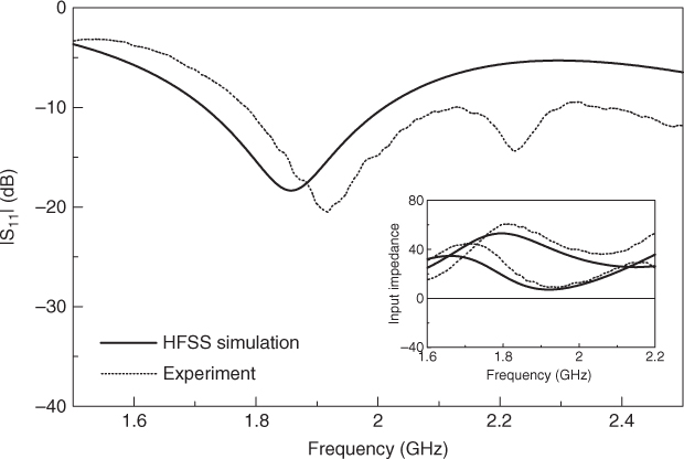
Figure 6.26 Antenna gain measured for a rectangular DRA with an underlaid solar cell. (From (13), copyright © 2010 IEEE, with permission.)

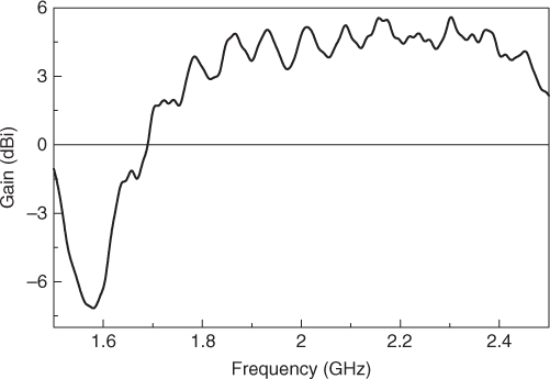
Figure 6.27 Normalized radiation patterns simulated and measured for a rectangular DRA with an underlaid solar cell: (a) E-plane; (b) H-plane. (From (13), copyright © 2010 IEEE, with permission.)

6.2.2.3 Optical Performances: Results and Discussion

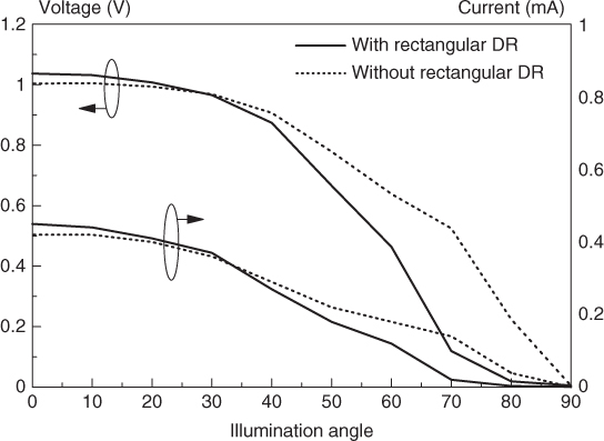
Figure 6.28 shows output voltages and currents measured using the same masked solar cell with R_c = 15 mm. The optical measurement setup shown in Fig. 6.16 is used again for the measurements. With reference to the figure, the rectangular DRA does not increase the outputs of the solar cell, suggesting that the rectangular DRA can be used for applications that do not want the focusing function. From the result, the focusing ability of the hemispherical DRA can be verified. Although the rectangular DRA does not provide a focusing function, its angular range for light reception is much wider than for its hemispherical counterpart. The output voltages and currents measured for R_c = 10 mm and 5 mm are also provided in Figs. 6.29 and 6.30, respectively. In general, the outputs do not degrade much for θ ≤ 40°, implying a larger light reception angle. Again, it is observed that larger illumination area generates higher voltage and current outputs, as expected.

Figure 6.28 Output voltages and currents of a solar cell with and without a rectangular DRA: R_c = 15 mm. (From (13), copyright © 2010 IEEE, with permission.)

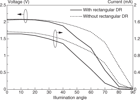
Figure 6.29 Output voltages and currents of a solar cell with and without a rectangular DRA: R_c = 10 mm.

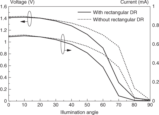
Figure 6.30 Output voltages and currents of a solar cell with and without a rectangular DRA: R_c = 5 mm.

6.3 Planar Solar-cell-integrated Antennas

In solar power plants, solar cells are often combined with light reflectors or concentrators to improve light-power utilization. The light-concentrating solar-cell array, called a heliostat (30), is frequently designed to track the movement of the sun. Traditionally, parabolic disks have been widely used as a solar concentrator to focus sunlight onto solar cells (31). With the use of solar concentrators, the light intensity at solar cells can be increased and thus a smaller number of photovoltaic cells can be used. In most cases, solar concentrators are made of silicon mirrors. Figure 6.31 shows parabolic and parallel-trench solar concentrators that are used for heating water. Of course, they can easily be modified into solar power plants by replacing the water containers with solar cells. As the making of a large-aperture parabolic structure can be mechanically challenging, smaller disks are usually cascaded instead to increase the solar power produced (32, 33). Nowadays, various sun-tracking mechanisms (32–34) are deployed to further increase the solar power efficiency of concentrator-type solar plants. Figure 6.32 shows an open-loop sun-tracking system (32) which can provide an output power of 35.7 kW/h per day. It has a total reflective area of 25 m². In recent years, to simplify the mechanical design, planar mirrors have been explored as solar concentrators (35). A solar plant designed by combining 360 pieces of nonimaging planar mirrors is shown in Fig. 6.33. It has a total area of 5760 cm² and is able to generate a temperature of 1084°C at the focal point of the parabolic disk. The National Renewable Energy Laboratory in the United States has estimated that a reflector-type power plant would be able to produce electricity at the very low cost of 5.49 cents/kWh by 2020, making solar power one of the cheapest renewable energies in the future (36).

Figure 6.31 Two different solar concentrators: (a) parabolic; (b) parallel trench. (Courtesy of S. L. Lau and K. K. Chong, Universiti Tunku Abdul Rahman, Malaysia.)

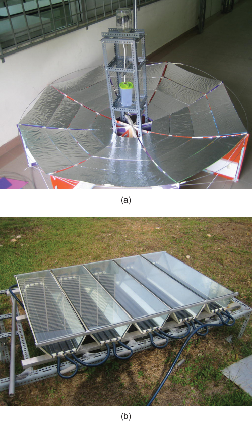
Figure 6.32 Open-loop sun-tracking heliostat designed by cascading many parabolic disks, giving a total reflective area of 25 m². (Courtesy of K. K. Chong, Universiti Tunku Abdul Rahman, Malaysia.)

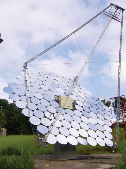
Figure 6.33 Solar plant with nonimaging planar mirrors. It is designed by cascading 360 pieces of planar mirrors, providing a total reflective area of 5760 cm². (Courtesy of K. K. Chong, Universiti Tunku Abdul Rahman, Malaysia.)

In this section, dual-functional antenna arrays that also serve as light concentrators or reflectors for solar cells are proposed. Since the idea is associated with renewable energy (37), a solar-cell-integrated antenna is also termed a green antenna. It will be shown that nonplanar ground planes, which are also light concentrators, are used for green antennas to provide the focusing effect. Instead of using silicon mirrors, metallic plates have been used, as they can easily be designed into electromagnetic radiators.

6.3.1 Solar-Cell-Integrated U-Shaped SPA

Because of their simple structure, wire antennas have been used extensively for many years. They were first utilized by Guglielmo Marconi in 1900 as signal-transmitting radiators. Over the past century, various wire antennas have been explored, such as the monopole, dipole, loop, spiral, and helix antennas. A simple wire antenna has an azimuthally omnidirectional radiation pattern. In 1995, Nakano et al. (38) showed that an L-shaped wire could be used as an efficient excitation probe for C-figured loop antennas. Later, Luk et al. (39) proposed an L-probe-fed suspended plate antenna (SPA). The SPA can provide a very wide impedance bandwidth of more than 35%, with stable radiation patterns across the entire passband. It also provides other advantages, such as low profile, light weight, and ease of excitation and tuning. SPA arrays were designed by Wong et al. (40) to increase the antenna gain. In this section, a U-shaped green antenna is demonstrated. The optical performances were evaluated by Lim et al. (41). It was found that using the U-shaped ground plane could increase the output voltage of solar cells significantly. Despite the introduction of solar cell panels, the antenna gain of the dual-functional SPA was not much affected.

6.3.1.1 Configuration

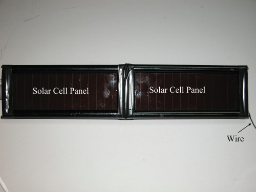
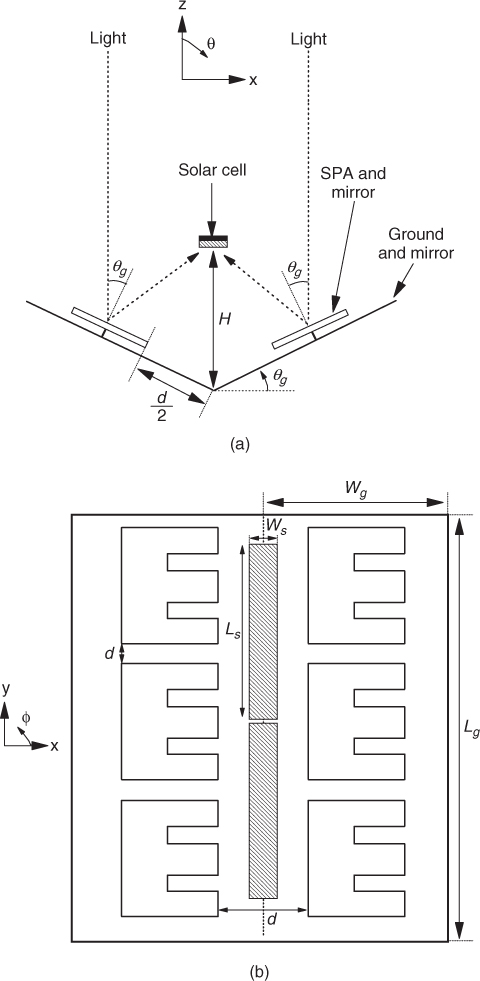
Figure 6.34 shows a single-element SPA fed by an L-probe. It will be used to design a solar-cell-integrated green antenna. The SPA was optimized at 2 GHz, with dimensions of L = 100 mm, W = 54 mm, H = 18 mm, t = 1.5 mm, L_h = 21.5 mm, and L_v = 11.9 mm. Next, the configuration of a green antenna is shown in Fig. 6.35. It is a 3 × 3 array consisting of nine SPA elements placed on a U-shaped ground plane, with parameters of d = 70 mm, W_g = 180 mm, L_g = 458 mm, and θ_g = 10°. The prototype, which is made of aluminum, is shown in Fig. 6.36. As the metallic surface can be scratched easily, such an antenna has to be handled carefully. Two one-sided amorphous solar-cell panels of W_s = 60 mm and L_s = 150 mm were used in our experiment. The solar cells are cascaded and connected electrically in parallel, as shown in Fig. 6.37. The solar cell panels were fixed using a polyvinyl chloride (PVC) holder at a height of H = 47 cm above the ground plane. Both the SPA elements and the ground plane can reflect sunlight to the solar-cell panels and thereby increase the output voltage of the solar system.

Figure 6.34 Single-element L-probe-fed SPA: (a) side view; (b) top view. (From (41), copyright © 2010 IEEE, with permission.)

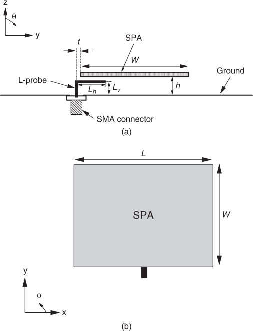
Figure 6.35 Solar concentrating green antenna consisting of a light-focusing 3 × 3 SPA array elements and two solar-cell panels suspended above a U-shaped ground plate: (a) front view; (b) top view. (From (41), copyright © 2010 IEEE, with permission.)

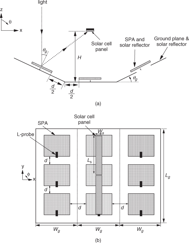
Figure 6.36 Green antenna: (a) front view; (b) top view.

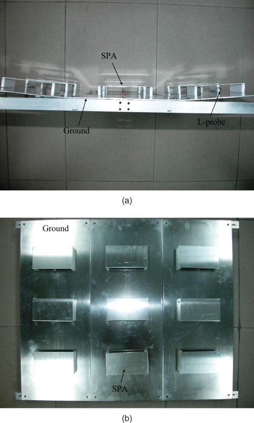
Figure 6.37 Cascaded solar cells.

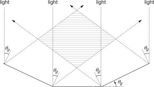
For ease of analyzing the light reflectivity of the ground plane, the suspended plates and solar cell panels are removed. As can be seen from Fig. 6.38, for normal light illumination the solar cells can be suspended at any point in the shaded region, which has a higher light intensity. Multiple solar-cell panels can be used for a larger electricity output. With reference to the figure, at normal light incident, it is observed that the central ground plate does not contribute much to the light beams directed to the solar cells.

Figure 6.38 Analysis of light beams above a U-shaped ground plate.

6.3.1.2 Antenna Performances: Results and Discussion

The antenna performance of a green antenna is discussed next. To begin, a single-element SPA (Fig. 6.34) resting on a 20 × 20 cm flat ground plane was optimized using Ansoft HFSS. Measurements were carried out using an Agilent 8753 network analyzer to verify the simulations. Figure 6.39 compares simulated and measured input impedances, where good agreement between the results is observed. The corresponding reflection coefficients are also shown in the inset. With reference to the inset, the antenna bandwidths measured and simulated (|S₁₁| ≤ − 10 dB) are about 38% and 42%, respectively. Two resonances are observed from the inset. The first resonance is caused by the TM₀₁ mode of the suspended plate, which can be verified easily by examining its electric field distribution. The resonance frequencies measured and simulated are 2.12 and 2.09 GHz (1.43% error), respectively. The second resonance is found at around 2.5 GHz. This mode should be caused by the L-probe because its frequency agrees reasonably well with 2.25 GHz, estimated using a primitive formula of f = c/4(L_v + L_h), where c is the speed of light in vacuum. The discrepancy between the two frequencies can be explained by the fact that the primitive formula does not take into account the effect of the suspended plate. In this section our attention is focused on the first (SPA) resonance mode only. Figure 6.40 shows the measured antenna gain of the SPA. With reference to the figure, the gain is about 7 dBi around the SPA mode. This value is typical for the dominant TM mode of the SPA (39). Figure 6.41 shows the radiation patterns of the SPA mode. Broadside patterns are found from the figure for both the E- and H-planes, as expected. With reference to the figure, the co-polarized fields are stronger than their cross-polarized counterparts by at least 20 dB in the boresight direction (θ = 0°). In the H-plane, the cross-polarization level increases with θ because of the current flowing on the horizontal arm of the L-probe (39). The simulated E-plane cross-polarized field is too minute to see in the figure.

Figure 6.39 Input impedances simulated and measured for a single-element SPA. The corresponding reflection coefficients are shown in the inset. (From (41), copyright © 2010 IEEE, with permission.)

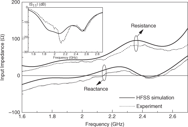
Figure 6.40 Antenna gain measured for a single-element SPA. (From (41), copyright © 2010 IEEE, with permission.)

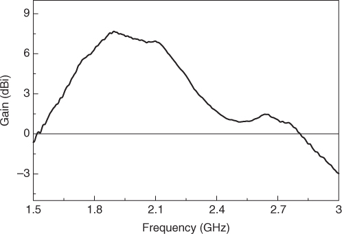
Figure 6.41 Normalized radiation patterns simulated and measured for a single-element SPA: (a) E-plane; (b) H-plane. (From (41), copyright © 2010 IEEE, with permission.)

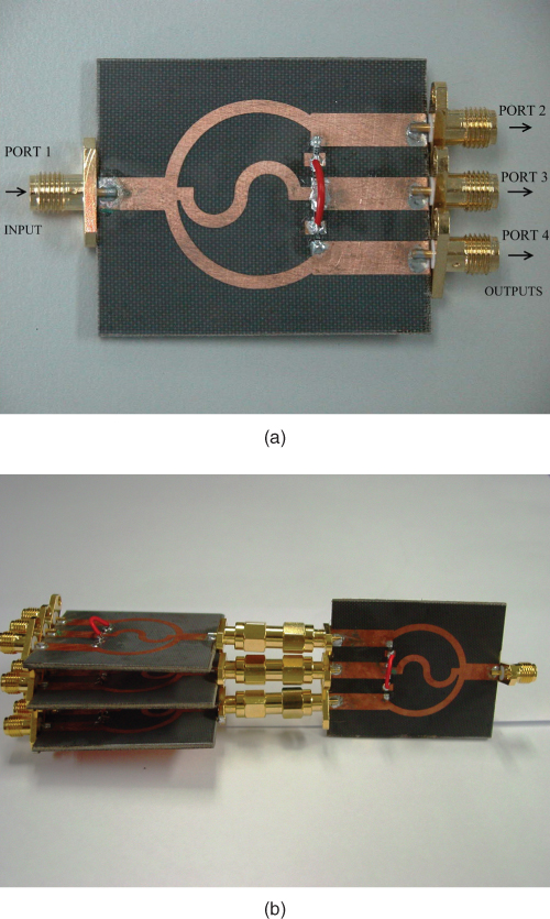
To feed the SPA array elements of a green antenna, four one-to-three-way Wilkinson power dividers were fabricated and cascaded. Figure 6.42 shows photographs of the Wilkinson power dividers. Four power dividers are cascaded [Fig. 6.42(b)] to feed the nine ports of the SPA array. Its design methodology can be found in (42). The magnitude passband measured for the power divider is from 1.45 to 2.23 GHz (|S_i1| ≤ 4.77 ± 0.5 dB, i = 2, 3, or 4), giving a bandwidth of 0.78 GHz. The phase bandwidth measured (|∠S_i1 − ∠S_j1| < 5°, i ≠ j and i, j > 1) is given by 2 GHz (1 to 3 GHz), which is much wider than the magnitude bandwidth. Obviously, the overall bandwidth of the power divider is limited by its magnitude response.

Figure 6.42 One-to-three Wikinson power dividers: (a) single piece; (b) in cascade. (From (41), copyright © 2010 IEEE, with permission.)

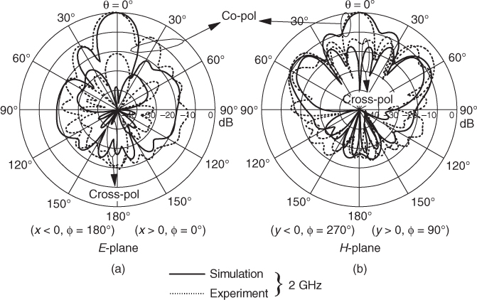
A green antenna is fabricated and tested after the SPA element and Wilkison power divider were designed. It is placed inside a far-field chamber (shown in Fig. 6.43) to measure the antenna gain and patterns. The solar cells are included so that their effects can be analyzed. The antenna gain measured is shown in Fig. 6.44. For ease of comparison, the antenna gain without solar-cell panels is also shown in the figure. As can be seen from Fig. 6.44, the antenna gain measured at 2 GHz is 15.2 dBi, which is only slightly lower than that without the solar-cell panels (15.5 dBi). It shows that the loss introduced by the panels is not very significant. The radiation patterns simulated and measured are shown in Fig. 6.45. It can be observed from the figure that for both E- and H-planes, the co-polarized fields are at least 15 dB stronger than the cross-polarized fields in the bore-sight direction. The cross-polarized field is stronger in the H-plane. Similar results were obtained for the flat ground plane case (40).

Figure 6.43 Green antenna placed in a far-field chamber with the solar cells suspended above it. (Measured at the State Key Laboratory of Millimeter Waves, City University of Hong Kong.)

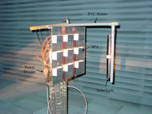
Figure 6.44 Antenna gain measured for a green antenna. The antenna gain measured for a green antenna without solar-cell panels is also shown. (From (41), copyright © 2010 IEEE, with permission.)

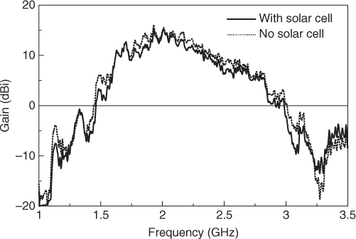
Figure 6.45 Normalized radiation patterns simulated and measured for a green antenna: (a) E-planel (b) H-plane. (From (41), copyright © 2010 IEEE, with permission.)

6.3.1.3 Optical Performances: Results and Discussion

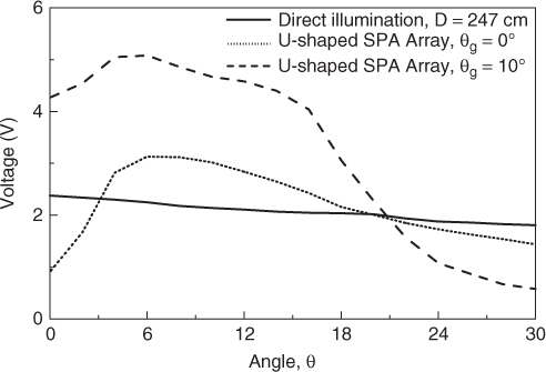
The optical performance of a green antenna is discussed next. It was placed on a rotator to measure the output voltage of the solar-cell panels at different illumination angles (θ). A xenon light source was used in our optical measurements. Figure 6.46 shows the experimental setup. The xenon light source has a wide spectrum and can mimic natural daylight. A parabolic optical dish was used to reflect the light from the source and generate a nearly parallel light beam. Its circular aperture has a diameter of 60 cm. Although an optical lens can produce a much better parallel light beam (13), it is difficult to obtain such a big lens commercially. The height H was found experimentally by optimizing the voltage output of the solar-cell panels at θ = 0°. Figure 6.47 shows photographs of the optical setup inside an optical dark room and a parabolic optical dish, respectively. Figrue 6.48 shows the output voltages of its solar-cell panels for θ_g = 0° (flat ground plane) and 10° (U-shaped ground plane), with H = 47 cm. It can be seen from the figure that when θ ≤ 22°, a larger output voltage is obtained using the U-shaped ground plane, due to its focusing effect. When the light is incident normally (θ = 0°), the output voltages are 4.27 and 0.91 V for the U-shaped and flat ground plane cases, respectively. It was found that an output voltage of 2.38 V is generated when the solar-cell panels are illuminated by the light source directly. In this case, for a fair comparison, the solar-cell panels were placed facing the light beam at a new distance that gives the same total path length (∼247 cm). It is interesting to note that the maximum output voltage of a green antenna is found at θ = 6° instead of θ = 0°. This is caused by the net effect of diffractions, reflections, and light blockage due to the solar-cell panels.

Figure 6.46 Top view of an experimental setup for optical measurements. (From (41), copyright © 2010 IEEE, with permission.)

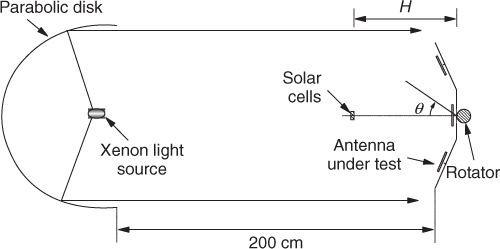
Figure 6.47 (a) Experimental setup inside an optical dark room. (b) Parabolic optical dish with a xenon light source. (From (41), copyright © 2010 IEEE, with permission.)

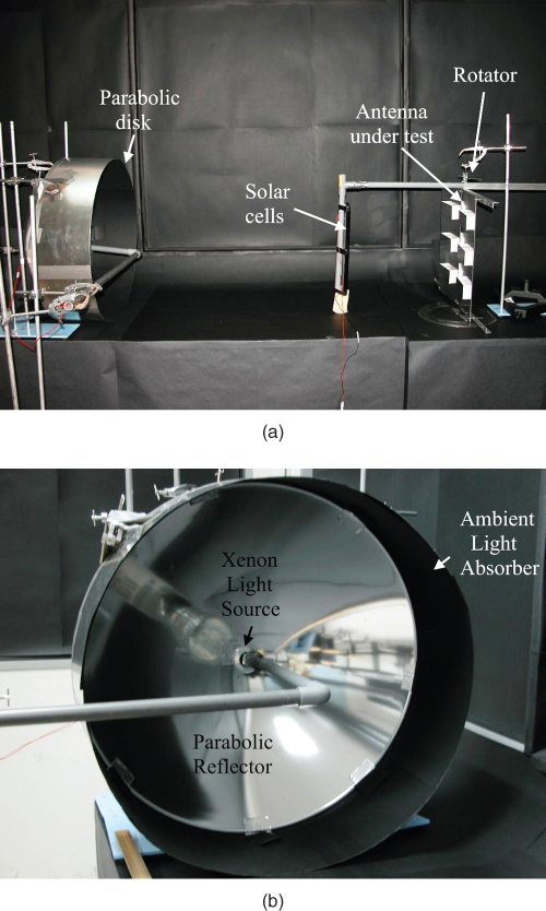
Figure 6.48 Output voltages of the solar-cell panels of a Green Antenna versus illumination angles (θ). (From (41), copyright © 2010 IEEE, with permission.)

6.3.2 Solar-Cell-Integrated V-Shaped SPA

In this section, six E-shaped patches are incorporated with a V-shaped ground plane and two solar-cell panels for designing a dual-functional antenna. This type of antenna was first published in a paper by Yang et al. (44). Like the antenna discussed in the preceding section, the antenna can be used for focusing sunlight onto solar cells.

6.3.2.1 Configuration

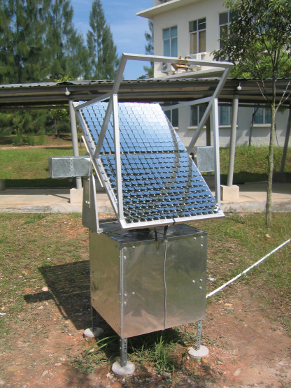
Figure 6.49 shows the configuration of a single-element E-shaped patch antenna (W₁ = 105 mm, W₂ = 36 mm, W₃ = 21 mm, H₁ = 67.5 mm, H₂ = 52.5 mm, t = 10.5 mm, and h = 15 mm). This antenna is used to design the light-focusing E-shaped patch array shown in Fig. 6.50. As can be seen from the figure, the antenna is a 3 × 2 array consisting of six E-shaped patches that are evenly placed on a V-shaped ground plane. Other design parameters are W_g = 162.5 mm, L_g = 590 mm, W_s = 60 mm, L_s = 150 mm, H = 55.7 mm, d = 94 mm, and θ_g = 5°. Several Wilkinson power dividers have been designed using the method of Maurin and Wu (42) to feed the antenna array at 1.6 GHz.

Figure 6.49 Single-element E-shaped patch antenna: (a) front view; (b) top view. (From (43), copyright © 2010 IEEE, with permission.)

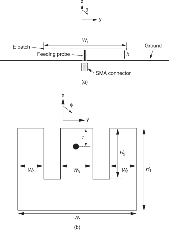
Figure 6.50 Light-focusing E-shaped patch array with two solar-cell panels suspended above a V-shaped ground plane: (a) front view; (b) top view. (From (43), copyright © 2010 IEEE, with permission.)

6.3.2.2 Antenna Performances: Results and Discussion

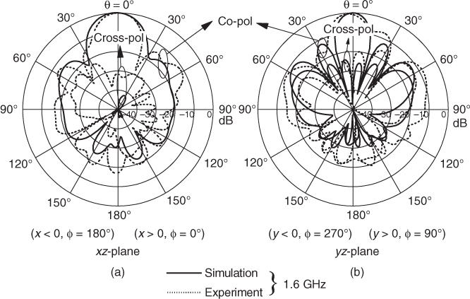
Figure 6.51 shows the reflection coefficients simulated and measured for a single-element patch antenna, and their corresponding input impedances are shown in the inset. Two resonant modes were measured at 1.5 GHz (a simulated value of 1.53 GHz) and 1.74 GHz (a simulated value of 1.76 GHz). The impedance bandwidth measured is about 25.3%, which is very close to the simulated value of 25.5%. The antenna gain measured for the light-reflecting E-shaped patch array (Fig. 6.50) is shown in Fig. 6.52. For comparison, the antenna gain for the same array was also measured with the solar cells removed. It can be observed that the solar cells do not introduce much loss to the antenna gain at 1.6 GHz. With reference to the figure, the antenna gain for the array with θ_g = 0° is also given. It is obvious that the solar cells cause the antenna gain of the second mode to degrade. The radiation patterns of the E-shaped patch array (θ_g = 5° with solar cells) are shown in Fig. 6.53. Broadside patterns are observed, with the co-polarized fields larger than their cross-polarized counterpart by at least 20 dBi in the bore-sight direction.

Figure 6.51 Reflection coefficients simulated and measured for a single-element E-shaped patch antenna. The corresponding input impedances are shown in the inset. (From (43), copyright © 2010 IEEE, with permission.)

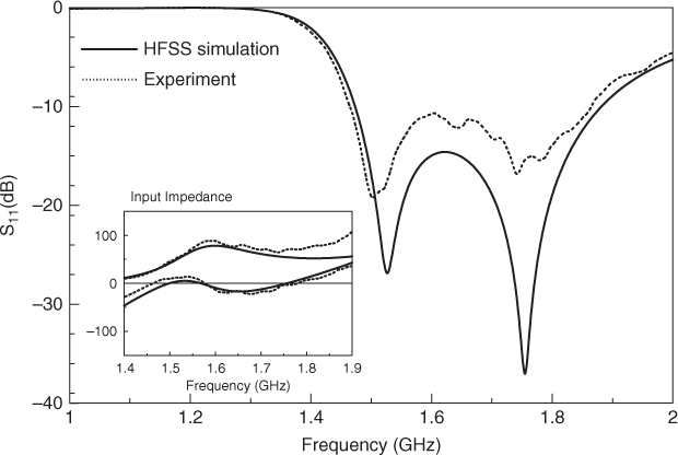
Figure 6.52 Antenna gain measured for an E-shaped patch array. The antenna gain measured for the same array without the solar cells is also shown. The results are compared to that for θ_g = 0°. (From (43), copyright © 2010 IEEE, with permission.)

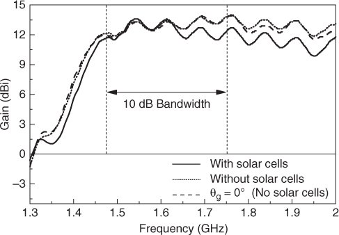
Figure 6.53 Normalized radiation patterns simulated and measured for an E-shaped patch array (θ_g = 5° with solar cells): (a) E-plane; (b) H-plane. (From (43), copyright © 2010 IEEE, with permission.)

6.3.2.3 Optical Performances: Results and Discussion

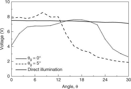
The same optical measurement setup (shown in Figs. 6.46 and 6.47) is used again for the experiments. It was found that when the light is incident normally (θ = 0°), output voltage with θ_g = 5° is higher than for θ_g = 0° by 102% (Fig. 6.54). This shows that the V-shaped patch array provides a good focusing effect. Also shown in the figure is the output voltage of the solar cells, being placed at a new distance (255.7 cm) so that it has an optical path identical to that for the inclined array. With reference to the figure, the focusing effect is found for θ ≤ 13° when θ_g = 5°.

Figure 6.54 Output voltages of solar cell panels of a solar-cell-integrated E-shaped patch versus illumination angles (θ). (From (43), copyright © 2010 IEEE, with permission.)

6.4 Conclusions

Several planar and nonplanar solar-cell-integrated antennas have been discussed in this chapter. Sometimes, designs of such a multifunctional module can be a trade-off between the performances of antenna and solar-cell systems. In the past, solar-cell-integrated antennas were used only in space-related applications. Recently, this technology has quietly come into terrestrial civilian lives (13, 45). By using solar-cell-integrated antennas, wireless systems with self-sustaining power sources can be obtained.

References

1. M. Tanaka, Y. Suzuki, K. Araki, and R. Suzuki, Microstrip antenna with solar cells for microsatellites, Electron. Lett., vol. 31, no. 1, pp. 5–6, Jan. 1995.

2. S. Vaccaro, J. R. Mosig, and P. D. Maagt, Two advanced solar antenna ‘Solant’ designs for satellite and terrestrial communications, IEEE Trans. Antennas Propagat., vol. 51, pp. 2028–2034, Aug. 2003.

3. S. Vaccaro, P. Torres, J. R. Mosig, A. Shah, J. F. Zurcher, A. K. Skrivervik, P. D. Maagt, and L. Gerlach, Stainless steel slot antenna with integrated solar cells, Electron. Lett., vol. 36, no. 25, pp. 2059–2060, Dec. 2000.

4. S. Vaccaro, C. Pereira, J. R. Mosig, and P. D. Maagt, In-flight experiment for combined planar antennas and solar cells (Solant), IET Microwave Antennas Propag., vol. 3, no. 8, pp. 1279–1287, 2009.

5. http://en.wikipedia.org/wiki/Satellite.

6. S. Vaccaro, J. R. Mosig, and P. D. Maagt, Making planar antennas out of solar cells, Electron. Lett., vol. 38, no. 17, pp. 945–947, Aug. 2002.

7. F. Kustas, “Semiconductor antenna array and solar energy collection assembly for spacecraft,” U.S. patent 6,087,991, July 11, 2001.

8. S. U. Hwu, B. P. Lu, L. A. Johnson, J. S. Fournet, R. J. Panneton, and G. D. Arndt, Scattering properties of solar panels for antenna pattern analysis, IEEE International Symposium on Antennas and Propagation Digest, 1994, vol. 1, pp. 266–269.

9. M. Tomisawa and M. Tokuda, “Induction characteristics of a solar cell to radiated electromagnetic disturbances,” Asia-Pacific Symposium on Electromagnetic Compatibility and 19th International Zurich Symposium on Electromagnetic Compatibility, 2008, pp. 538–541.

10. S. V. Shynu, M. J. R. Ons, P. McEvoy, M. J. Ammann, S. J. McCormack, and B. Norton, Integration of microstrip patch antenna with polycrystalline silicon solar cell, IEEE Trans. Antennas Propag., vol. 57, pp. 3969–3972, Dec. 2009.

11. S. V. Shynu, M. J. Ammann, and B. Norton, Quarter-wave metal plate solar antenna, Electron. Lett., vol. 44, no. 9, pp. 570–571, Apr. 2008

12. S. V. Shynu, M. J. R. Ons, G. Ruvio, M. J. Ammann, S. McCormack, and B. Norton, “A microstrip printed dipole solar antenna using polycrystalline silicon solar cells,” IEEE International Symposium on Antennas and Propagation and USNC/URSI National Radio Science Meeting, July 5–11, San Diego, CA, 2008.

13. E. H. Lim and K. W. Leung, Transparent dielectric resonator antennas for optical applications, IEEE Trans. Antennas Propag., vol. 58, pp. 1054–1059, Apr. 2010.

14. M. J. R. Ons, S. V. Shynu, M. J. Ammann, S. J. McCormack, and B. Norton, Emitter-wrap-through photovoltaic dipole antenna with solar concentrator, Electron. Lett., vol. 45, no. 5, pp. 241–242, Feb. 2009.

15. T. W. Turpin and R. Baktur, Meshed patch antennas integrated on solar cells, IEEE Antennas Wireless Propag. Lett., vol. 8, pp. 693–696, June 2009.

16. K. M. Luk and K. W. Leung, Eds., Dielectric Resonator Antennas. London: Research Studies Press, 2003.

17. A. Petosa, Dielectric Resonator Antenna Handbook. Norwood, MA: Artech House, 2007.

18. A. K. Skrivervik, J. F. Zurcher, O. Staub, and J. R. Mosig, PCS antenna design: the challenge of miniaturization, IEEE Antennas Propag. Mag., vol. 43, no. 4, pp. 13–27, Aug. 2001.

19. http://www.camglassblowing.co.uk/gproperties.

20. K. W. Leung, K. M. Luk, K. Y. A. Lai, and D. Lin, Theory and experiment of a coaxial probe fed dielectric resonator antenna, IEEE Trans. Antennas Propag., vol. 41, pp. 1390–1398, Oct. 1993.

21. K. W. Leung, K. M. Luk, K. Y. A. Lai, and D. Lin, Theory and experiment of an aperture-coupled hemispherical dielectric resonator antenna, IEEE Trans. Antennas Propag., vol. 43, pp. 1192–1198, Nov. 1995.

22. A. A. Kishk, G. Zhou, and A. W. Glisson, Analysis of dielectric resonator antennas with emphasis on hemispherical structures, IEEE Antennas Propag. Mag., vol. 36, no. 2, pp. 20–31, Apr. 1994.

23. K. W. Leung, Conformal strip excitation of dielectric resonator antenna, IEEE Trans. Antennas Propag., vol. 48, pp. 961–967, June 2000.

24. Datasheet: Borosilicate Glass Properties.

25. J. Dheepa, R. Sathyamoorthy, A. Subbarayan, S. Velumani, P. J. Sebastian, and R. Perez, Dielectric properties of vacuum deposited Bi2Te3 thin films, Solar Energy Mater. Solar Cells, vol. 88, no. 2, pp. 187–198, July 2005.

26. G. P. Junker, A. A. Kishk, A. W. Glisson, and D. Kajfez, Effect of an air gap around the coaxial probe exciting a cylindrical dielectric resonator antenna, Electron. Lett., vol. 30, no. 3, pp. 177–178, 1994.

27. G. P. Junker, A. A. Kishk, A. W. Glisson, and D. Kajfez, Effect of an air gap on a cylindrical dielectric resonator antennas operating in the TM₀₁ mode, Electron. Lett., vol. 30, no. 2, pp. 97–98, 1994.

28. S. M. Shum and K. M. Luk, Characteristics of dielectric ring resonator antenna with an air gap, Electron. Lett., vol. 30, pp. 277–278, Feb. 1994.

29. E. Hecht, Optics, 4th ed. Reading, MA: Addison Wesley, 2002.

30. W. B. Stine and R. W. Halligan, Eds, Solar Energy Fundamentals and Design with Computer Applications. New York: Wiley, 1985, pp. 135–262.

31. R. B. Diver and T. A. Moss, Practical field alignment of parabolic trough solar concentrators, J. Solar Energy Eng., vol. 129, pp. 153–159, May 2007.

32. K. K. Chong, C. Wong, F. Siaw, T. Yew, S. Ng, M. Liang, Y. Lim, and S. Lau, Integration of an on-axis general sun-tracking formula in the algorithm of an open-loop sun-tracking system, Sensors, vol. 9, pp. 7849–7865, Sept. 2009.

33. K. K. Chong, Optimization of nonimaging focusing heliostat in dynamic correction of astigmatism for a wide range of incidence angles, Opt. Lett., vol. 35, no. 10, pp. 1614–1616, 2010.

34. K. K. Chong, Optical analysis for simplified astigmatic correction of non-imaging focusing heliostat, Solar Energy, vol. 84, pp. 1356–1365, 2010.

35. K. K. Chong, F. Siaw, C. Wong, and G. Wong, Design and construction of non-imaging planar concentrator for concentrator photovoltaic system, Renewable Energy, vol. 34, pp. 1364–1370, 2009.

36. Report: Assessment of Parabolic Trough and Power Tower Solar Technology Cost and Performance Forecasts, NREL/SR-550-34440, Oct. 2003.

37. http://en.wikipedia.org/wiki/Sustainable_energy#Green_energy.

38. H. Nakano, H. Yoshisda, and Y. Wu, C-figured loop antennas, Electron. Lett., vol. 31, no. 9, pp. 693–694, Apr. 1995.

39. K. M. Luk, C. L. Mak, Y. L. Chow, and K. F. Lee, Broadband microstrip patch antenna, Electron. Lett., vol. 34, no. 15, pp. 1442–1443, July 1998.

40. H. Wong, K. L. Lau, and K. W. Luk, Design of dual-polarized L-probe patch antenna arrays with high isolation, IEEE Trans. Antennas Propag., vol. 52, pp. 45–52, Jan. 2004.

41. E. H. Lim, K. W. Leung, S. C. Su, and H. Y. Wong, Green antenna for solar energy collection, IEEE Antennas Wireless Propag. Lett., vol. 9, pp. 689–692, July 2010.

42. D. Maurin and K. Wu, A compact 1.7–2.1GHz three-way power combiner using microstrip technology with better than 93.8% combining efficiency, IEEE Microwave Guided Wave Lett., vol. 6, pp. 106–109, Feb. 1996.

43. E. H. Lim, K. W. Leung, G. H. Khor, and K. K. Chan, “A solar power plant with light-reflecting E-shaped patch antenna,” IEEE International Symposium on Antennas and Propagation and USNC/URSI National Radio Science Meeting 2010, Toronto, Oatario, Canada, July 11–17, 2010.

44. F. Yang, X. Zhang, X. Ye, and Y. Rahmat-Samii, Wide-band E-shaped patch antennas for wireless communications, IEEE Trans. Antennas Propag., vol. 49, pp. 1094–1100, July 2001.

45. T. Schuetze, H. Hullmann, and C. Bendel, “Multifunctional photovoltaic building design and efficient photovoltaic use of solar energy,” World Climate & Energy Event, Rio de Janeiro, Brazil, Mar. 17–19, 2009.