Chapter 11: Diagnosing Problems

Finally, after instrumenting application code, configuring a collector to transmit the data, and setting up a backend to receive the telemetry, we have all the pieces in place to observe a system. But what does that mean? How can we detect abnormalities in a system with all these tools? That's what this chapter is all about. This chapter aims to look through the lens of an analyst and see what the shape of the data looks like as events occur in a system. To do this, we'll look at the following areas:

• How leaning on chaos engineering can provide the framework for running experiments in a system
• Common scenarios of issues that can arise in distributed systems
• Tools that allow us to introduce failures into our system

As we go through each scenario, we'll describe the experiment, propose a hypothesis, and use telemetry to verify whether our expectations match what the data shows us. We will use the data and become more familiar with analysis tools to help us understand how we may answer questions about our systems in production. As always, let's start by setting up our environment first.

Technical requirements

The examples in this chapter will use the grocery store application we've used and revisited throughout the book. Since the chapter's goal is to analyze telemetry and not specifically look at how this telemetry is produced, the application code will not be the focus of the chapter. Instead of running the code as separate applications, we will use it as Docker (https://docs.docker.com/get-docker/) containers and run it via Compose. Ensure Docker is installed with the following command:

$ docker version

Client:

Cloud integration: 1.0.14

Version:           20.10.6

API version:       1.41

Go version:        go1.16.3 ...

The following command will ensure Docker Compose is also installed:

$ docker compose version

Docker Compose version 2.0.0-beta.1

The book's companion repository (https://github.com/PacktPublishing/Cloud-Native-Observability) contains the Docker Compose configuration file, as well as the configuration required to run the various containers. Download the companion repository via Git:

$ git clone https://github.com/PacktPublishing/Cloud-Native-Observability

$ cd Cloud-Native-Observability/chapter11

With the configuration in place, start the environment via the following:

$ docker compose up

Throughout the chapter, as we conduct experiments, know that it is always possible to reset the pristine Docker environment by removing the containers entirely with the following commands:

$ docker compose stop

$ docker compose rm

All the tools needed to run various experiments have already been installed inside the grocery store application containers, meaning there are no additional tools to install. The commands will be executed via docker exec and run within the container.

Introducing a little chaos

In normal circumstances, the real world is unpredictable enough that intentionally introducing problems may seem unnecessary. Accidental configuration changes, sharks chewing through undersea cables, and power outages affecting data centers are just a few events that have caused large-scale issues across the world. In distributed systems, in particular, dependencies can cause failures that may be difficult to account for during normal development.

Putting applications through various stress, load, functional, and integration tests before they are deployed to production can help predict their behavior to a large extent. However, some circumstances may be hard to reproduce outside of a production environment. A practice known as chaos engineering (https://principlesofchaos.org) allows engineers to learn and explore the behavior of a system. This is done by intentionally introducing new conditions into the system through experiments. The goal of these experiments is to ensure that systems are robust enough to withstand failures in production.

Important Note

Although chaos engineers run experiments in production, it's essential to understand that one of the principles of chaos engineering is not to cause unnecessary pain to users, meaning experiments must be controlled and limited in scope. In other words, despite its name, chaos engineering isn't just going around a data center and unplugging cables haphazardly.

The cycle for producing experiments goes as follows:

1. It begins with a system under a known good state or steady state.
2. A hypothesis is then proposed to explain the experiment's impact on the system's state.
3. The proposed experiment is run on the system.
4. Verification of the impact on the system takes place, validating that the prediction matches the hypothesis. The verification step provides an opportunity to identify unexpected side effects of the experiment. If something behaved precisely as expected, great! If it acted worse than expected, why? If it behaved better than expected, what happened? It's essential to understand what happened, especially if the results were better than expected. It's too easy to look at a favorable outcome and move right along without taking the time to understand why it happened.
5. Once verification is complete, improvements to the system are made, and the cycle begins anew. Ideally, running these experiments can be automated once the results on the system are satisfactory to guard against future regressions.

Figure 11.1 – Chaos engineering life cycle

The hypothesis step is crucial because if the proposed experiment will have disastrous repercussions on the system, it may be worth rethinking the experiment.

For example, a hypothesis that turning off all production servers simultaneously will cause a complete system failure doesn't need to be validated. Additionally, this would guarantee the creation of unnecessary pain for all users of the system. There isn't much to learn from running this in production, except seeing how quickly users send angry tweets.

An alternative experiment that may be worthwhile is to shut down an availability zone or a region of a system to ensure load balancing works. This would provide an opportunity to learn how production traffic would be handled in the case of such a failure, validating that those systems in place to manage such a failure are doing their jobs. Of course, if no such mechanisms are in place, it's not worth experimenting either, as this would have the same impact as shutting down all the servers for all users in that zone or region.

This chapter will take a page out of the chaos engineering book and introduce various failure modes into the grocery store system. We will propose a hypothesis and run experiments to validate the assumptions. Using the telemetry produced by the store, we will validate that the system behaved as expected. This will allow us to use the telemetry produced to understand how we can answer questions about our system via this information. Let's explore a problem that impacts all networked applications: latency.

Experiment #1 – increased latency

Latency is the delay introduced when a call is made and the response is returned to the originating caller. It can inject itself into many aspects of a system. This is especially true in a distributed system where latency can be found anywhere one service calls out to another. The following diagram shows an example of how latency can be calculated between two services. Service A calls a remote service (B), the request duration is 25 ms, but a large portion of that time is spent transferring data to and from service B, with only 5 ms spent executing code.

Figure 11.2 – Latency incurred by calling a remote service

If the services are collocated, the latency is usually negligible and can often be ignored. However, latency must be accounted for when services communicate over a network. This is something to think about at development time. It can be caused by factors such as the following:

• The physical distance between the servers hosting services. As even the speed of light requires time to travel distance, the greater the distance between services, the greater the latency.
• A busy network. If a network reaches the limits of how much data it can transfer, it may throttle the data transmitted.
• Problems in any applications or systems connecting the services. Load balancers and DNS services are just two examples of the services needed to connect two services.

Experiment

The first experiment we'll run is to increase the latency in the network interface of the grocery store. The experiment uses a Linux utility to manipulate the configuration on the network interface: Traffic Control (https://en.wikipedia.org/wiki/Tc_(Linux)). Traffic Control, or tc, is a powerful utility that can simulate a host of scenarios, including packet loss, increased latency, or throughput limits. In this experiment, tc will add a delay to inbound and outbound traffic, as shown in Figure 11.3:

Figure 11.3 – Experiment #1 will add latency to the network interface

Hypothesis

Increasing the latency to the grocery store network interface will incur the following:

• A reduction in the total number of requests processed
• An increase in the request duration time

Use the following Docker command to introduce the latency. This uses the tc utility inside the grocery store container to add a 1s delay to all traffic received and sent through interface eth0:

$ docker exec grocery-store tc qdisc add dev eth0 root netem delay 1s

Verify

To observe the metrics and traces generated, access the Application Metrics dashboard in Grafana via the following URL: http://localhost:3000/d/apps/application-metrics. You'll immediately notice a drop in the Request count time series and an increase in Request duration time quantiles. As time passes, you'll also start seeing the Request duration distribution histogram change to show an increasing number of requests falling into buckets with longer durations that are as per the following screenshot:

Figure 11.4 – Request metrics for shopper, grocery-store, and inventory services

Note that although the drop in request count is the same across the inventory and grocery store services, the duration of the request for the inventory service remains unchanged. This is a great starting point, but it would be ideal to identify precisely where this jump in the request duration occurred.

Important Note

As discussed earlier in this book, the correlation between metrics and traces provided by exemplars could help us drill down more quickly by giving us specific traces to investigate from the metrics. However, since the implementation of exemplar support in OpenTelemetry is still under development at the time of writing, the example in this chapter does not take advantage of it. I hope that by the time you're reading this, exemplar support is implemented across many languages in OpenTelemetry.

Let's look at the tracing data in Jaeger available at http://localhost:16686. From the metrics, we already know that the issue appears to be isolated to the grocery store service. Sure enough, searching for traces for that service yields the following chart:

Figure 11.5 – Increased duration results in Jaeger

It's clear from this chart that something happened. The following screenshot shows us two traces; at the top is a trace from before we introduced the latency; at the bottom is a trace from after. Although the two look similar, looking at the duration of the spans named web request and /products, it's clear that those operations are taking far longer at the bottom than at the top.

Figure 11.6 – Trace comparison before and after latency was introduced

As hypothesized, the total number of requests processed by the grocery store dropped due to the simulation. This, in turn, reduced the number of calls to the inventory service. The total duration of the request as observed by the shopper client increased significantly.

Remove the delay to see how the system recovers. The following command removes the delay introduced earlier:

$ docker exec grocery-store tc qdisc del dev eth0 root netem delay 1s

Latency is only one of the aspects of networks that can cause problems for applications. Traffic Control's network emulator (https://man7.org/linux/man-pages/man8/tc-netem.8.html) functionality can simulate many other symptoms, such as packet loss and rate-limiting, or even the re-ordering of packets. If you're keen on playing with networks, it can be a lot of fun to simulate different scenarios. However, the network isn't the only thing that can cause problems for systems.

Experiment #2 – resource pressure

Although cloud providers make provisioning new computing resources more accessible than ever before, even computing in the cloud is still bound by the physical constraints of hardware running applications. Memory, processors, hard drives, and networks all have their limits. Many factors can contribute to resource exhaustion:

• Misconfigured or misbehaving applications. Crashing and restarting in a fast loop, failing to free memory, or making requests over the network too aggressively can all contribute to a load on resources.
• An increase or spike in requests being processed by the service. This could be good news; the service is more popular than ever! Or it could be bad news, the result of a denial-of-service attack. Either way, more data to process means more resources are required.
• Shared resources cause resource starvation. This problem is sometimes referred to as the noisy neighbor problem, where resources are consumed by another tenant of the physical hardware where a service is running.

Autoscaling or dynamic resource allocation helps alleviate resource pressures to some degree by allowing users to configure thresholds at which new resources should be made available to the system. To know how these thresholds should be configured, it's valuable to experiment with how applications behave under limited resources.

Experiment

We'll investigate how telemetry can help identify resource pressures in the following scenario. The grocery store container is constrained to 50 M of memory via its Docker Compose configuration. Memory pressure will be applied to the container via stress.

The Unix stress utility (https://www.unix.com/man-page/debian/1/STRESS/) spins workers that produce loads on systems. It creates memory, CPU, and I/O pressures by calling system functions in a loop; malloc/free, sqrt, and sync, depending on which resource is being pressured.

Figure 11.7 – Experiment #2 will apply memory pressure to the container

Hypothesis

As resources are consumed by stress, we expect the following to happen:

• The grocery store processes fewer requests as it cannot obtain the resources to process requests.
• Latency increases across the system, as requests will take longer to process through the grocery store.
• Metrics collected from the grocery store container should quickly identify the increased resource pressure.

The following introduces memory pressure by adding workers that consume a total of 40 M of memory to the grocery store container via stress for 30 minutes:

$ docker exec grocery-store stress --vm 20 --vm-bytes 2M --timeout 30m

stress: info: [20] dispatching hogs: 0 cpu, 0 io, 10 vm, 0 hdd

Verify

With the pressure in place, let's see whether the telemetry matches what we expected. Looking at the application metrics, we can see an almost immediate increase in request duration as per the following screenshot. The request count is also slightly impacted simultaneously.

Figure 11.8 – Application metrics

What else can we learn about the event? Searching through traces, an increase in duration similar to what occurred during the first experiment is shown:

Figure 11.9 – Trace duration increased

Looking in more detail at individual traces, we can identify which paths through the code cause this increase. Not surprisingly, the allocating memory span, which locates an operation performing a memory allocation, is now significantly longer, with its time jumping from 2.48 ms to 49.76 ms:

Figure 11.10 – Trace comparison before and after the memory increase

There is a second dashboard worth investigating at this time, the Container metrics dashboard (http://localhost:3000/d/containers/container-metrics). This dashboard shows the CPU, memory, and network metrics collected directly from Docker by the collector's Docker stats receiver (https://github.com/open-telemetry/opentelemetry-collector-contrib/tree/main/receiver/dockerstatsreceiver). Reviewing the following charts, it's evident that resource utilization increased significantly in one container:

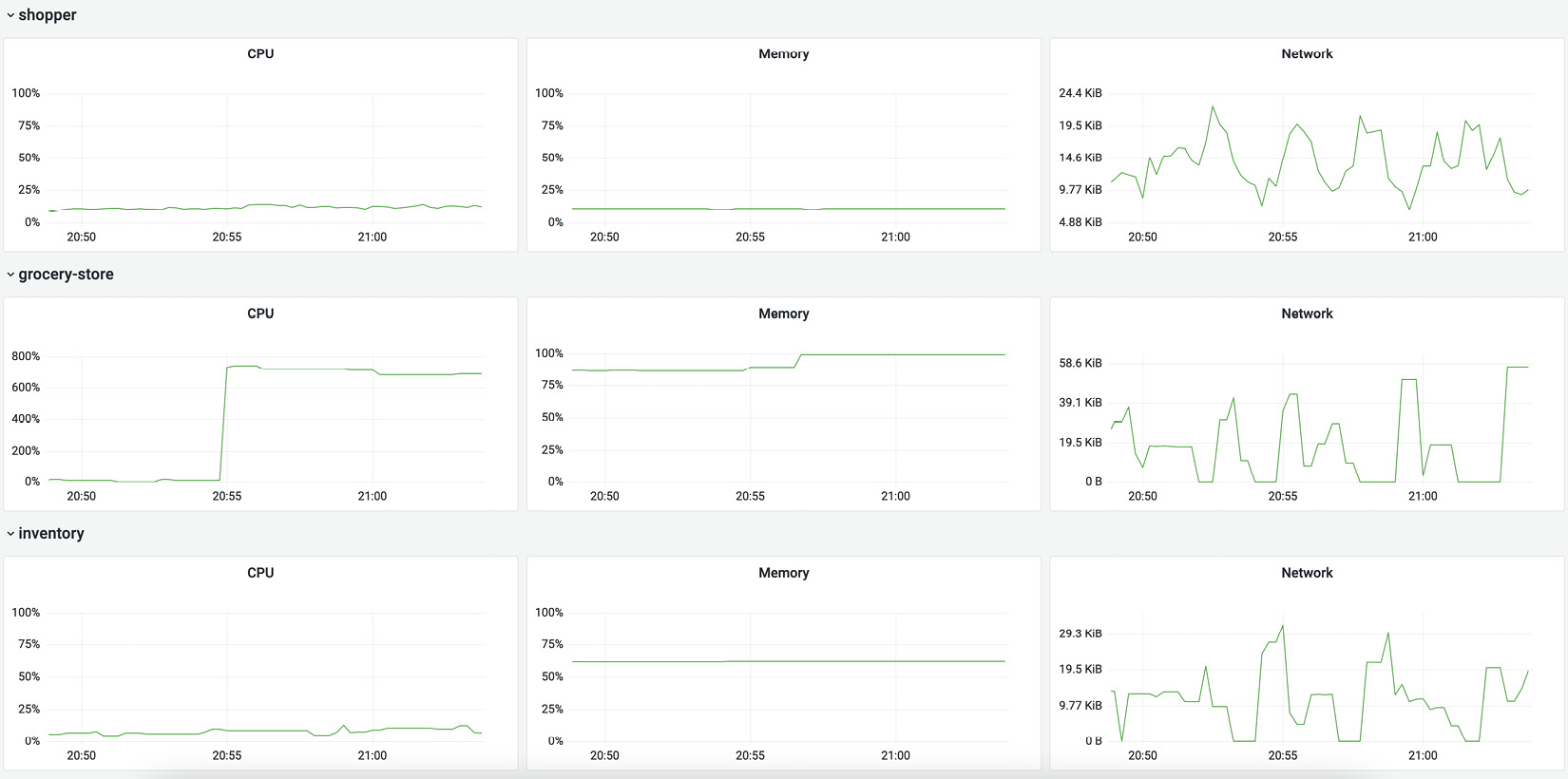
Figure 11.11 – Container metrics for CPU, memory, and network

From the data, it's evident that something happened to the container running the grocery store. The duration of requests through the system increased, as did the metrics showing memory and CPU utilization for the container. Identifying resource pressure in this testing environment isn't particularly interesting beyond this.

Recall that OpenTelemetry specifies resource attributes for all signals, meaning that if multiple services are running on the same resource, host, container, or node, it would be possible to correlate information about those services using this resource information, meaning that if we were running multiple applications on the same host, and one of them triggered memory pressure, it would be possible to verify its impact on other services within the same host by utilizing its resource attributes as an identifier when querying telemetry.

Resource information can help answer questions when, for example, a host has lost power, and there is a need to identify all services impacted by this event quickly. Another way to use this information is when two completely unrelated services are experiencing problems simultaneously. If those two services operate on the same node, resource information will help connect the dots.

Experiment #3 – unexpected shutdown

If a service exits in a forest of microservices and no one is around to observe it, does it make a sound? With the right telemetry and alert configuration in place, it certainly does. Philosophical questions aside, services shutting down happens all the time. Ensuring that services can manage this event gracefully is vital in dynamic environments where applications come and go as needed.

Expected and unexpected shutdowns or restarts can be caused by any number of reasons. Some common ones are as follows:

• An uncaught exception in the code causes the application to crash and exit.
• Resources consumed by a service pass a certain threshold, causing an application to be terminated by a resource manager.
• A job completes its task, exiting intentionally as it terminates.

Experiment

This last experiment will simulate a service exiting unexpectedly in our system to give us an idea of what to look for when identifying this type of failure. Using the docker kill command, the inventory service will be shut down unexpectedly, leaving the rest of the services to respond to this failure and report this issue.

Figure 11.12 – Experiment #3 will terminate the inventory service

In a production environment, issues arising from this scenario would be mitigated by having multiple instances of the inventory service running behind some load balancing, be it a load balancer or DNS load balancing. This would result in traffic being redirected away from the failed instance and over to the others still in operation. For our experiment, however, a single instance is running, causing a complete failure of the service.

Hypothesis

Shutting down the inventory service will result in the following:

• All metrics from the inventory container will stop reporting.
• Errors will be recorded by the grocery store; this should be visible through the request count per status code reporting status code 500.
• Logs should report errors from the shopper container.

Using the following command, send a signal to shut down the inventory service. Note that docker kill sends the container a kill signal, whereas docker stop would send a term signal. We use kill here to prevent the service from shutting down cleanly:

$ docker kill inventory

Verify

With the inventory service stopped, let's head over to the application metrics dashboard one last time to see what happened. The request count graph shows a rapid increase in requests whose response code is 500, representing an internal server error.

Figure 11.13 – The request counter shows an increase in errors

One signal we've yet to use in this chapter is logging. Look for the Logs panel at the bottom of the application metrics dashboard to find all the logs emitted by our system. Specifically, look for an entry reporting a failed request to the grocery store such as the following, which is produced by the shopper application:

Figure 11.14 – Log entry being recorded

Expanding the log entry shows details about the event that caused an error. Unfortunately, the message request to grocery store failed isn't particularly helpful here, although notice that there is a TraceID field in the data shown. This field is adjacent to a link. Clicking on the link will take us to the corresponding trace in Jaeger, which shows us the following:

Figure 11.15 – Trace confirms the grocery store is unable to contact the inventory

The trace provides more context as to what error caused it to fail, which is helpful. An exception with the message recorded in the span provides ample details about the legacy-inventory service appearing to be missing. Lastly, the container metrics dashboard will confirm the inventory container stopped reporting metrics as per the following screenshot:

Figure 11.16 – Inventory container stopped reporting metrics

Restore the stopped container via the docker start command and observe as the error rate drops and traffic is returned to normal:

$ docker start inventory

There are many more scenarios that we could investigate in this chapter. However, we only have limited time to cover these. From message queues filling up to caching problems, the world is full of problems just waiting to be uncovered.

Using telemetry first to answer questions

These experiments are a great way to gain familiarity with telemetry. Still, it feels like cheating to know what caused a change before referring to the telemetry to investigate a problem. A more common way to use telemetry is to look at it when a problem occurs without intentionally causing it. Usually, this happens when deploying new code in a system.

Code changes are deployed to many services in a distributed system several times a day. This makes it challenging to figure out which change is responsible for a regression. The complexity of identifying problematic code is compounded by the updates being deployed by different teams. Update the image configuration for the shopper, grocery-store, and legacy-inventory services in the Docker Compose configuration to use the following:

docker-compose.yml

  shopper:

    image: codeboten/shopper:chapter11-example1

...

  grocery-store:

    image: codeboten/grocery-store:chapter11-example1

...

  legacy-inventory:

    image: codeboten/legacy-inventory:chapter11-example1

Update the containers by running the following command in a separate terminal:

$ docker compose up -d legacy-inventory grocery-store shopper

Was the deployment of the new code a success? Did we make things better or worse? Let's look at what the data shows us. Starting with the application metrics dashboard, it doesn't look promising. Request duration has spiked upward, and requests per second dropped significantly.

Figure 11.17 – Application metrics of the deployment

It appears to be impacting both the inventory service and grocery store service, which would indicate something may have gone wrong in the latest deployment of the inventory service. Looking at traces, searching for all traces shows the same increase in request duration as the graphs from the metrics. Selecting a trace and looking through the details points to a likely culprit:

Figure 11.18 – A suspicious span named sleepy service

It appears the addition of an operation called sleepy service is causing all sorts of problems in the latest deployment! With this information, we can revert the change and resolve the issue.

In addition to the previous scenario, four additional scenarios are available through published containers to practice your observation skills. They have unoriginal tags: chapter11-example2, chapter11-example3, chapter11-example4, and chapter11-example5. I recommend trying them all before looking through the scenarios folder in the companion repository to see whether you can identify the deployed problem!

Summary

Learning to navigate telemetry data produced by systems comfortably takes time. Even with years of experience, the most knowledgeable engineers can still be puzzled by unexpected changes in observability data. The more time spent getting comfortable with the tools, the quicker it will be to get to the bottom of just what caused changes in behavior.

The tools and techniques described in this chapter can be used repeatedly to better understand exactly what a system is doing. With chaos engineering practices, we can improve the resilience of our systems by identifying areas that can be improved upon under controlled circumstances. By methodically experimenting and observing the results from our hypotheses, we can measure the improvements as we're making them.

Many tools are available for experimenting and simulating failures; learning how to use these tools can be a powerful addition to any engineer's toolset. As we worked our way through the vast amount of data produced by our instrumented system, it's clear that having a way to correlate data across signals is critical in quickly moving through the data.

It's also clear that generating more data is not always a good thing, as it is possible to become overwhelmed quickly or overwhelm backends. The last chapter looks at how sampling can help reduce the volume of data.