Chapter 5: Metrics – Recording Measurements
Tracing code execution throughout a system is one way to capture information about what is happening in an application, but what if we're looking to measure something that would be better served by a more lightweight option than a trace? Now that we've learned how to generate distributed traces using OpenTelemetry, it's time to look at the next signal: metrics. As we did in Chapter 4, Distributed Tracing – Tracing Code Execution, we will first look at configuring the OpenTelemetry pipeline to produce metrics. Then, we'll continue to improve the telemetry emitted by the grocery store application by using the instruments OpenTelemetry puts at our disposal. In this chapter, we will do the following:
- Configure OpenTelemetry to collect, aggregate, and export metrics to the terminal.
- Generate metrics using the different instruments available.
- Use metrics to gain a better understanding of the grocery store application.
Augmenting the grocery store application will allow us to put the different instruments into practice to grasp better how each instrument can be used to record measurements. As we explore other metrics that are useful to produce for cloud-native applications, we will seek to understand some of the questions we may answer using each instrument.
Technical requirements
As with the examples in the previous chapter, the code is written using Python 3.8, but OpenTelemetry Python supports Python 3.6+ at the time of writing. Ensure you have a compatible version installed on your system following the instructions at https://docs.python.org/3/using/index.html. To verify that a compatible version is installed on your system, run the following commands:
$ python --version
$ python3 --version
On many systems, both python and python3 point to the same installation, but this is not always the case, so it's good to be aware of this if one points to an unsupported version. In all examples, running applications in Python will call the python command, but they can also be run via the python3 command, depending on your system.
The first few examples in this chapter will show a standalone example exploring how to configure OpenTelemetry to produce metrics. The code will require the OpenTelemetry API and SDK packages, which we'll install via the following pip command:
$ pip install opentelemetry-api==1.10.0
opentelemetry-sdk==1.10.0
opentelemetry-propagator-b3==1.10.0
Additionally, we will use the Prometheus exporter to demonstrate a pull-based exporter to emit metrics. This exporter can be installed via pip as well:
$ pip install opentelemetry-exporter-prometheus==0.29b0
For the later examples involving the grocery store application, you can download the sample from Chapter 4, Distributed Tracing – Tracing Code Execution, and add the code along with the examples. The following git command will clone the companion repository:
$ git clone https://github.com/PacktPublishing/Cloud-Native-Observability
The chapter04 directory in the repository contains the code for the grocery store. The complete example, including all the code in the examples from this chapter, is available in the chapter05 directory. I recommend adding the code following the examples and using the complete example code as a reference if you get into trouble. Also, if you haven't read Chapter 4, Distributed Tracing – Tracing Code Execution, it may be helpful to skim through the details of how the grocery store application is built in that chapter to get your bearings.
The grocery store depends on the Requests library (https://docs.python-requests.org/) to make web requests at various points and the Flask library (https://flask.palletsprojects.com) to provide a lightweight web server for some of the services. Both libraries can be installed via the following pip command:
$ pip install flask requests
Additionally, the chapter will utilize a third-party open source tool (https://github.com/rakyll/hey) to generate some load on the web application. The tool can be downloaded from the repository. The following commands download the macOS binary and rename it to hey using curl with the -o flag, then ensure the binary is executable using chmod:
$ curl -o hey https://hey-release.s3.us-east-2.amazonaws.com/hey_darwin_amd64
$ chmod +x ./hey
If you have a different load generation tool you're familiar with, and there are many, feel free to use that instead if you prefer. This should be everything we need to start; let's start measuring!
Configuring the metrics pipeline
The metrics signal was designed to be conceptually similar to the tracing signal. The metrics pipeline consists of the following:
- A MeterProvider to determine how metrics should be generated and provide access to a meter.
- The meter is used to create instruments, which are used to record measurements.
- Views allow the application developer to filter and process metrics produced by the software development kit (SDK).
- A MetricReader, which collects metrics being recorded.
- The MetricExporter provides a mechanism to translate metrics into an output format for various protocols.
There are quite a few components, and a picture always helps me grasp concepts more quickly. The following figure shows us the different elements in the pipeline:

Figure 5.1 – Metrics pipeline
MeterProvider can be associated with a resource to identify the source of metrics produced. We'll see shortly how we can reuse the LocalMachineResourceDetector we created in Chapter 4, Distributed Tracing – Tracing Code Execution, with metrics. For now, the first example instantiates MeterProvider with an empty resource. The code then calls the set_meter_provider global method to set the MeterProvider for the entire application.
Add the following code to a new file named metrics.py. Later in the chapter, we will refactor the code to add a MeterProvider to the grocery store, but to get started, the simpler, the better.
metrics.py
from opentelemetry._metrics import set_meter_provider
from opentelemetry.sdk._metrics import MeterProvider
from opentelemetry.sdk.resources import Resource
def configure_meter_provider():
provider = MeterProvider(resource=Resource.create())
set_meter_provider(provider)
if __name__ == "__main__":
configure_meter_provider()
Run the code with the following command to ensure it runs without any errors:
python ./metrics.py
No errors and no output? Well done, you're on the right track!
Important Note
The previous code shows that the metric modules are located at _metrics. This will change to metrics once the packages have been marked stable. Depending on when you're reading this, it may have already happened.
Next, we'll need to configure an exporter to tell our application what to do with metrics once they're generated. The OpenTelemetry SDK contains ConsoleMetricExporter that emits metrics to the console, useful when getting started and debugging. PeriodicExportingMetricReader can be configured to periodically export metrics. The following code configures both components and adds the reader to the MeterProvider. The code sets the export interval to 5000 milliseconds, or 5 seconds, overriding the default of 60 seconds:
metrics.py
from opentelemetry._metrics import set_meter_provider
from opentelemetry.sdk._metrics import MeterProvider
from opentelemetry.sdk.resources import Resource
from opentelemetry.sdk._metrics.export import (
ConsoleMetricExporter,
PeriodicExportingMetricReader,
)
def configure_meter_provider():
exporter = ConsoleMetricExporter()
reader = PeriodicExportingMetricReader(exporter, export_interval_millis=5000)
provider = MeterProvider(metric_readers=[reader], resource=Resource.create())
set_meter_provider(provider)
if __name__ == "__main__":
configure_meter_provider()
Run the code once more. The expectation is that the output from running the code will still not show anything. The only reason to run the code is to ensure our dependencies are fulfilled, and there are no typos.
Important Note
Like TracerProvider, MeterProvider uses a default no-op implementation in the API. This allows developers to instrument code without worrying about the details of how metrics will be generated. It does mean that unless we remember to set the global MeterProvider to use MeterProvider from the SDK package, any calls made to the API to generate metrics will result in no metrics being generated. This is one of the most common gotchas for folks working with OpenTelemetry.
We're almost ready to start producing metrics with an exporter, a metric reader, and a MeterProvider configured. The next step is getting a meter.
Obtaining a meter
With MeterProvider globally configured, we can use a global method to obtain a meter. As mentioned earlier, the meter will be used to create instruments, which will be used throughout the application code to record measurements. The meter receives the following arguments at creation time:
- The name of the application or library generating metrics
- An optional version identifies the version of the application or library producing the telemetry
- An optional schema_url to describe the data generated
Important Note
The schema URL was introduced in OpenTelemetry as part of the OpenTelemetry Enhancement Proposal 152 (https://github.com/open-telemetry/oteps/blob/main/text/0152-telemetry-schemas.md). The goal of schemas is to provide OpenTelemetry instrumented applications a way to signal to external systems consuming the telemetry what the semantic versioning of the data produced will look like. Schema URL parameters are optional but recommended for all producers of telemetry: meters, tracers, and log emitters.
This information is used to identify the application or library producing the metrics. For example, application A making a web request via the requests library may contain more than one meter:
- The first meter is created by application A with a name identifying it with the version number matching the application.
- A second meter is created by the requests instrumentation library with the name opentelemetry-instrumentation-requests and the instrumentation library version.
- The urllib instrumentation library creates the third meter with the name opentelemetry-instrumentation-urllib, a library utilized by the requests library.
Having a name and a version identifier is critical in differentiating the source of the metrics. As we'll see later in the chapter, when we look at the Views section, this identifying information can also be used to filter out the telemetry we're not interested in. The following code uses the get_meter_provider global API method to access the global MeterProvider we configured earlier, and then calls get_meter with a name, version, and schema_url parameter:
metrics.py
from opentelemetry._metrics import get_meter_provider, set_meter_provider
...
if __name__ == "__main__":
configure_meter_provider()
meter = get_meter_provider().get_meter(
name="metric-example",
version="0.1.2",
schema_url=" https://opentelemetry.io/schemas/1.9.0",
)
In OpenTelemetry, instruments used to record measurements are associated with a single meter and must have unique names within the context of that meter.
Push-based and pull-based exporting
OpenTelemetry supports two methods for exporting metrics data to external systems: push-based and pull-based. A push-based exporter sends measurements from the application to a destination at a regular interval on a trigger. This trigger could be a maximum number of metrics to transfer or a schedule. The push-based method will be familiar to users of StatsD (https://github.com/statsd/statsd), where a network daemon opens a port and listens for metrics to be sent to it. Similarly, the ConsoleSpanExporter for the tracing signal in Chapter 4, Distributed Tracing – Tracing Code Execution, is a push-based exporter.
On the other hand, a pull-based exporter exposes an endpoint pulled from or scraped by an external system. Most commonly, a pull-based exporter exposes this information via a web endpoint or a local socket; this is the method popularized by Prometheus (https://prometheus.io). The following diagram shows the data flow comparison between a push and a pull model:

Figure 5.2 – Push versus pull-based reporting
Notice the direction of the arrow showing the interaction between the exporter and an external system. When configuring a pull-based exporter, remember that system permissions may need to be configured to allow an application to open a new port for incoming requests. One such pull-based exporter defined in the OpenTelemetry specification is the Prometheus exporter.
The pipeline configuration for a pull exporter is slightly less complex. The metric reader interface can be used as a single point to collect and expose metrics in the Prometheus format. The following code shows how to expose a Prometheus endpoint on port 8000 using the start_http_server method from the Prometheus client library. It then configures PrometheusMetricReader with a prefix parameter to provide a namespace for all metrics generated by our application. Finally, the code adds a call waiting for input from the user before exiting; this gives us a chance to see the exposed metrics before the application exits:
from opentelemetry.exporter.prometheus import PrometheusMetricReader
from prometheus_client import start_http_server
def configure_meter_provider():
start_http_server(port=8000, addr="localhost")
reader = PrometheusMetricReader(prefix="MetricExample")
provider = MeterProvider(metric_readers=[reader], resource=Resource.create())
set_meter_provider(provider)
if __name__ == "__main__":
...
input("Press any key to exit...")
If you run the application now, you can use a browser to see the Prometheus formatted data available by visiting http://localhost:8000. Alternatively, you can use the curl command to see the output data in the terminal as per the following example:
$ curl http://localhost:8000
# HELP python_gc_objects_collected_total Objects collected during gc
# TYPE python_gc_objects_collected_total counter
python_gc_objects_collected_total{generation="0"} 1057.0
python_gc_objects_collected_total{generation="1"} 49.0
python_gc_objects_collected_total{generation="2"} 0.0
# HELP python_gc_objects_uncollectable_total Uncollectable object found during GC
# TYPE python_gc_objects_uncollectable_total counter
python_gc_objects_uncollectable_total{generation="0"} 0.0
python_gc_objects_uncollectable_total{generation="1"} 0.0
python_gc_objects_uncollectable_total{generation="2"} 0.0
# HELP python_gc_collections_total Number of times this generation was collected
# TYPE python_gc_collections_total counter
python_gc_collections_total{generation="0"} 55.0
python_gc_collections_total{generation="1"} 4.0
python_gc_collections_total{generation="2"} 0.0
# HELP python_info Python platform information
# TYPE python_info gauge
python_info{implementation="CPython",major="3",minor="8",patchlevel="0",version="3.9.0"} 1.0
The Prometheus client library generates the previous data; note that there are no OpenTelemetry metrics generated by our application, which makes sense since we haven't generated anything yet! We'll get to that next. We'll see in Chapter 11, Diagnosing Problems, how to integrate OpenTelemetry with a Prometheus backend. For the sake of simplicity, the remainder of the examples in this chapter will be using the push-based ConsoleMetricExporter configured earlier. If you're more familiar with Prometheus, please use this configuration instead.
Choosing the right OpenTelemetry instrument
We're now ready to generate metrics from our application. If you recall, in tracing, the tracer produces spans, which are used to create distributed traces. By contrast, the meter does not generate metrics; an instrument does. The meter's role is to produce instruments. OpenTelemetry offers many different instruments to record measurements. The following figure shows a list of all the instruments available:

Figure 5.3 – OpenTelemetry instruments
Each instrument has a specific purpose, and the correct instrument depends on the following:
- The type of measurement being recorded
- Whether the measurement must be done synchronously
- Whether the values being recorded are monotonic or not
For synchronous instruments, a method is called on the instrument when it is time for a measurement to be recorded. For asynchronous instruments, a callback method is configured at the instrument's creation time.
Each instrument has a name and kind property. Additionally, a unit and a description may be specified.
Counter
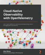
A counter is a commonly available instrument across metric ecosystems and implementations over the years, although its definition across systems varies. In OpenTelemetry, a counter is an increasing monotonic instrument, only supporting non-negative value increases. The following diagram shows a sample graph representing a monotonic counter:
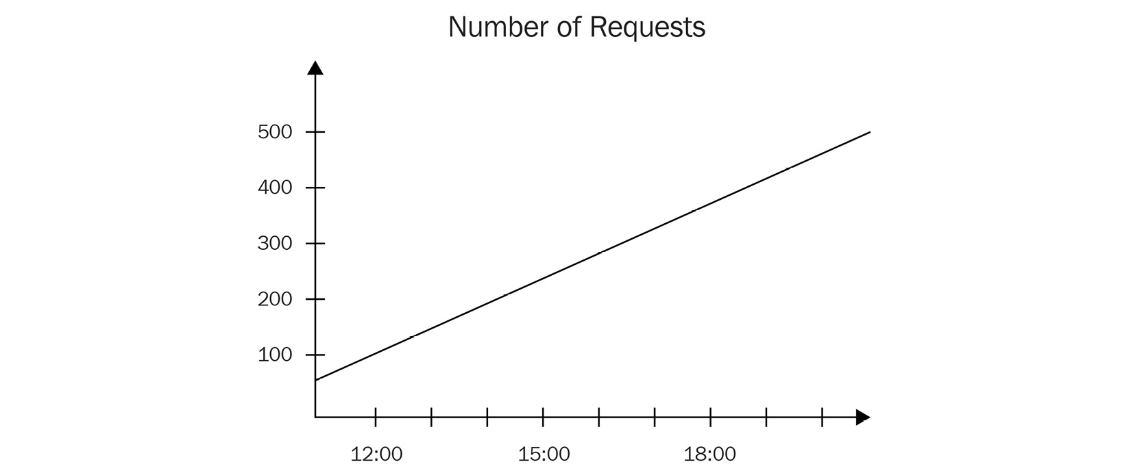
Figure 5.4 – Increasing monotonic counter graph
A counter can be used to represent the following:
- Number of requests received
- Count of orders processed
- CPU time utilization
The following code instantiates a counter to keep a tally of the number of items sold in the grocery store. The code uses the add method to increment the counter and passes the locale of the customer as an attribute:
metrics.py
if __name__ == "__main__":
...
counter = meter.create_counter(
"items_sold",
unit="items",
description="Total items sold"
)
counter.add(6, {"locale": "fr-FR", "country": "CA"})
counter.add(1, {"locale": "es-ES"})
Running the code outputs the counter with all its attributes:
output
{"attributes": {"locale": "fr-FR", "country": "CA"}, "description": "Total items sold", "instrumentation_info": "InstrumentationInfo(metric-example, 0.1.2, https://opentelemetry.io/schemas/1.9.0)", "name": "items_sold", "resource": "BoundedAttributes({'telemetry.sdk.language': 'python', 'telemetry.sdk.name': 'opentelemetry', 'telemetry.sdk.version': '1.10.0', 'service.name': 'unknown_service'}, maxlen=None)", "unit": "items", "point": {"start_time_unix_nano": 1646535699616146000, "time_unix_nano": 1646535699616215000, "value": 7, "aggregation_temporality": 2, "is_monotonic": true}}
{"attributes": {"locale": "es-ES"}, "description": "Total items sold", "instrumentation_info": "InstrumentationInfo(metric-example, 0.1.2, https://opentelemetry.io/schemas/1.9.0)", "name": "items_sold", "resource": "BoundedAttributes({'telemetry.sdk.language': 'python', 'telemetry.sdk.name': 'opentelemetry', 'telemetry.sdk.version': '1.10.0', 'service.name': 'unknown_service'}, maxlen=None)", "unit": "items", "point": {"start_time_unix_nano": 1646535699616215001, "time_unix_nano": 1646535699616237000, "value": 0, "aggregation_temporality": 2, "is_monotonic": true}}
Note that the attributes themselves do not influence the value of the counter. They are only augmenting the telemetry with additional dimensions about the transaction. A monotonic instrument like the counter cannot receive a negative value. The following code tries to add a negative value:
if __name__ == "__main__":
...
counter.add(6, {"locale": "fr-FR", "country": "CA"})
counter.add(-1, {"unicorn": 1})
This code results in the following warning, which provides the developer with a helpful hint:
output
Add amount must be non-negative on Counter items_sold.
Knowing to use the right instrument can help avoid generating unexpected data. It's also good to consider adding validation to the data being passed into instruments when unsure of the data source.
Asynchronous counter
The asynchronous counter can be used as a counter. Its only difference is that it is used asynchronously. Asynchronous counters can represent data that is only ever-increasing, and that may be too costly to report synchronously or is more appropriate to record on set intervals. Some examples of this would be reporting the following:
- CPU time utilized by a process
- Total network bytes transferred
The following code shows us how to create an asynchronous counter using the async_counter_callback callback method, which will be called every time PeriodExportingMetricReader executes. To ensure the instrument has a chance to record a few measurements, we've added sleep in the code as well to pause the code before exiting:
metrics.py
import time
from opentelemetry._metrics.measurement import Measurement
def async_counter_callback():
yield Measurement(10)
if __name__ == "__main__":
...
# async counter
meter.create_observable_counter(
name="major_page_faults",
callback=async_counter_callback,
description="page faults requiring I/O",
unit="fault",
)
time.sleep(10)
If you haven't commented out the output from the instrument, you should see the output from both counters now. The following output omits the previous example's output for brevity:
output
{"attributes": "", "description": "page faults requiring I/O", "instrumentation_info": "InstrumentationInfo(metric-example, 0.1.2, https://opentelemetry.io/schemas/1.9.0)", "name": "major_page_faults", "resource": "BoundedAttributes({'telemetry.sdk.language': 'python', 'telemetry.sdk.name': 'opentelemetry', 'telemetry.sdk.version': '1.10.0', 'service.name': 'unknown_service'}, maxlen=None)", "unit": "fault", "point": {"start_time_unix_nano": 1646538230507539000, "time_unix_nano": 1646538230507614000, "value": 10, "aggregation_temporality": 2, "is_monotonic": true}}
{"attributes": "", "description": "page faults requiring I/O", "instrumentation_info": "InstrumentationInfo(metric-example, 0.1.2, https://opentelemetry.io/schemas/1.9.0)", "name": "major_page_faults", "resource": "BoundedAttributes({'telemetry.sdk.language': 'python', 'telemetry.sdk.name': 'opentelemetry', 'telemetry.sdk.version': '1.10.0', 'service.name': 'unknown_service'}, maxlen=None)", "unit": "fault", "point": {"start_time_unix_nano": 1646538230507539000, "time_unix_nano": 1646538235507059000, "value": 20, "aggregation_temporality": 2, "is_monotonic": true}}
These counters are great for ever-increasing values, but measurements go up and down sometimes. Let's see what OpenTelemetry has in store for that.
An up/down counter
The following instrument is very similar to the counter. As you may have guessed from its name, the difference between the counter and the up/down counter is that the latter can record values that go up and down; it is non-monotonic. The following diagram shows us what a graph representing a non-monotonic counter may look like:

Figure 5.5 – Non-monotonic counter graph
Creating an UpDownCounter instrument is done via the create_up_down_counter method. Increment and decrement operations are done via the single add method with either positive or negative values:
metrics.py
if __name__ == "__main__":
...
inventory_counter = meter.create_up_down_counter(
name="inventory",
unit="items",
description="Number of items in inventory",
)
inventory_counter.add(20)
inventory_counter.add(-5)
The previous example's output will be as follows:
output
{"attributes": "", "description": "Number of items in inventory", "instrumentation_info": "InstrumentationInfo(metric-example, 0.1.2, https://opentelemetry.io/schemas/1.9.0)", "name": "inventory", "resource": "BoundedAttributes({'telemetry.sdk.language': 'python', 'telemetry.sdk.name': 'opentelemetry', 'telemetry.sdk.version': '1.10.0', 'service.name': 'unknown_service'}, maxlen=None)", "unit": "items", "point": {"start_time_unix_nano": 1646538574503018000, "time_unix_nano": 1646538574503083000, "value": 15, "aggregation_temporality": 2, "is_monotonic": false}}
Note the previous example only emits a single metric. This is expected as the two recordings were aggregated into a single value for the period reported.
Asynchronous up/down counter
As you may imagine, as the counter has an asynchronous counterpart, so does UpDownCounter. The asynchronous up/down counter allows us to increment or decrement a value on a set interval. As you will see shortly, it is pretty similar in nature to the asynchronous gauge. The main difference between the two is that the asynchronous up/down counter should be used when the values being recorded are additive in nature, meaning the measurements can be added across dimensions. Some examples of metrics that could be recorded via this instrument are as follows:
- Changes in the number of customers in a store
- Net revenue for an organization across business units
The following creates an asynchronous up/down counter to keep track of the current number of customers in a store. Note that, unlike its synchronous counterpart, the value recorded in the asynchronous up/down counter is an absolute value, not a delta. As per the previous asynchronous example, an async_updowncounter_callback callback method does the work of reporting the measure:
metrics.py
def async_updowncounter_callback():
yield Measurement(20, {"locale": "en-US"})
yield Measurement(10, {"locale": "fr-CA"})
if __name__ == "__main__":
...
upcounter_counter = meter.create_observable_up_down_counter(
name="customer_in_store",
callback=async_updowncounter_callback,
unit="persons",
description="Keeps a count of customers in the store"
)
The output will start to look familiar based on the previous examples we've already run through:
output
{"attributes": {"locale": "en-US"}, "description": "Keeps a count of customers in the store", "instrumentation_info": "InstrumentationInfo(metric-example, 0.1.2, https://opentelemetry.io/schemas/1.9.0)", "name": "customer_in_store", "resource": "BoundedAttributes({'telemetry.sdk.language': 'python', 'telemetry.sdk.name': 'opentelemetry', 'telemetry.sdk.version': '1.10.0', 'service.name': 'unknown_service'}, maxlen=None)", "unit": "persons", "point": {"start_time_unix_nano": 1647735390164970000, "time_unix_nano": 1647735390164986000, "value": 20, "aggregation_temporality": 2, "is_monotonic": false}}
{"attributes": {"locale": "fr-CA"}, "description": "Keeps a count of customers in the store", "instrumentation_info": "InstrumentationInfo(metric-example, 0.1.2, https://opentelemetry.io/schemas/1.9.0)", "name": "customer_in_store", "resource": "BoundedAttributes({'telemetry.sdk.language': 'python', 'telemetry.sdk.name': 'opentelemetry', 'telemetry.sdk.version': '1.10.0', 'service.name': 'unknown_service'}, maxlen=None)", "unit": "persons", "point": {"start_time_unix_nano": 1647735390164980000, "time_unix_nano": 1647735390165009000, "value": 10, "aggregation_temporality": 2, "is_monotonic": false}}
Counters and up/down counters are suitable for many data types, but not all. Let's see what other instruments allow us to measure.
Histogram
A histogram instrument is useful when comparing the frequency distribution of values across large data sets. Histograms use buckets to group the data they represent and effectively identify outliers or anomalies. Some examples of data representable by histograms are as follows:
- Response times for requests to a service
- The height of individuals
Figure 5.6 shows a sample histogram chart representing the response time for requests. It looks like a bar chart, but it differs in that each bar represents a bucket containing a range for the values it contains. The y axis represents the count of elements in each bucket:

Figure 5.6 – Histogram graph
To capture information in a histogram, the buckets specified must be able to contain all the values it expects to record. For example, take a histogram containing two buckets with explicit upper bounds of 0 ms and 10 ms. Any measurement greater than 10 ms bound would be excluded from the histogram. Both Prometheus and OpenTelemetry address this by capturing any value beyond the maximum upper boundary in an additional bucket. The histograms we'll explore in this chapter all use explicit boundaries, but OpenTelemetry also provides experimental support for exponential histograms (https://github.com/open-telemetry/opentelemetry-specification/blob/main/specification/metrics/datamodel.md#exponentialhistogram).
Histograms can be, and are often, used to calculate percentiles. The following code creates a histogram via the create_histogram method. The method used to produce a metric with a histogram is named record:
metrics.py
if __name__ == "__main__":
...
histogram = meter.create_histogram(
"response_times",
unit="ms",
description="Response times for all requests",
)
histogram.record(96)
histogram.record(9)
In this example, we record two measurements that fall into separate buckets. Notice how they appear in the output:
output
{"attributes": "", "description": "Response times for all requests", "instrumentation_info": "InstrumentationInfo(metric-example, 0.1.2, https://opentelemetry.io/schemas/1.9.0)", "name": "response_times", "resource": "BoundedAttributes({'telemetry.sdk.language': 'python', 'telemetry.sdk.name': 'opentelemetry', 'telemetry.sdk.version': '1.10.0', 'service.name': 'unknown_service'}, maxlen=None)", "unit": "ms", "point": {"start_time_unix_nano": 1646539219677439000, "time_unix_nano": 1646539219677522000, "bucket_counts": [0, 0, 1, 0, 0, 0, 1, 0, 0, 0, 0], "explicit_bounds": [0.0, 5.0, 10.0, 25.0, 50.0, 75.0, 100.0, 250.0, 500.0, 1000.0], "sum": 105, "aggregation_temporality": 2}}
As with the counter and up/down counter, the histogram is synchronous.
Asynchronous gauge
The last instrument defined by OpenTelemetry is the asynchronous gauge. This instrument can be used to record measurements that are non-additive in nature; in other words, which wouldn't make sense to sum together. An asynchronous gauge can represent the following:
- The average memory consumption of a system
- The temperature of a data center
The following code uses Python's built-in resource module to measure the maximum resident set size (https://en.wikipedia.org/wiki/Resident_set_size). This value is set in async_gauge_callback, which is used as the callback for the gauge we're creating:
metrics.py
import resource
def async_gauge_callback():
rss = resource.getrusage(resource.RUSAGE_SELF).ru_maxrss
yield Measurement(rss, {})
if __name__ == "__main__":
...
meter.create_observable_gauge(
name="maxrss",
unit="bytes",
callback=async_gauge_callback,
description="Max resident set size",
)
time.sleep(10)
Running the code will show us memory consumption information about our application using OpenTelemetry:
output
{"attributes": "", "description": "Max resident set size", "instrumentation_info": "InstrumentationInfo(metric-example, 0.1.2, https://opentelemetry.io/schemas/1.9.0)", "name": "maxrss", "resource": "BoundedAttributes({'telemetry.sdk.language': 'python', 'telemetry.sdk.name': 'opentelemetry', 'telemetry.sdk.version': '1.10.0', 'service.name': 'unknown_service'}, maxlen=None)", "unit": "bytes", "point": {"time_unix_nano": 1646539432021601000, "value": 18341888}}
{"attributes": "", "description": "Max resident set size", "instrumentation_info": "InstrumentationInfo(metric-example, 0.1.2, https://opentelemetry.io/schemas/1.9.0)", "name": "maxrss", "resource": "BoundedAttributes({'telemetry.sdk.language': 'python', 'telemetry.sdk.name': 'opentelemetry', 'telemetry.sdk.version': '1.10.0', 'service.name': 'unknown_service'}, maxlen=None)", "unit": "bytes", "point": {"time_unix_nano": 1646539437018742000, "value": 19558400}}
Excellent, we now know about the instruments and have started generating a steady metrics stream. The last topic about instruments to be covered is duplicate instruments.
Duplicate instruments
Duplicate instrument registration conflicts arise if more than one instrument is created within a single meter with the same name. This can potentially produce semantic errors in the data, as many telemetry backends uniquely identify metrics via their names. Conflicting instruments may be intentional when two separate code paths need to report the same metric, or, when multiple developers want to record different metrics but accidentally use the same name; naming things is hard. There are a few ways the OpenTelemetry SDK handles conflicting instruments:
- If the conflicting instruments are identical, the values recorded by these instruments are aggregated. The data generated appears as though a single instrument produced them.
- If the instruments are not identical, but the conflict can be resolved via View configuration, the user will not be warned. As we'll see next, views provide a mechanism to produce unique metric streams, differentiating the instruments.
- If the instruments are not identical and their conflicts are not resolved via views, a warning is emitted, and their data is generated without modification.
Individual meters act as a namespace, meaning two meters can separately create identical instruments without any issues. Using a unique namespace for each meter ensures that application developers can create instruments that make sense for their applications without running the risk of interfering with other metrics generated by underlying libraries. This will also make searching for metrics easier once exported outside the application. Let's see how we can shape the metrics stream to fit our needs with views.
Customizing metric outputs with views
Some applications may produce more metrics than an application developer is interested in. You may have noticed this with the example code for instruments; as we added more examples, it became difficult to find the metrics we were interested in. Recall the example mentioned earlier in this chapter: application A represents a client library making web requests that could produce metrics via three different meters. If each of those meters keeps a request counter, duplicate data is highly likely to be generated. Duplicated data may not be a problem on a small scale, but when scaling services up to handling thousands and millions of requests, unnecessary metrics can become quite expensive. Thankfully, views provide a way for users of OpenTelemetry to configure the SDK only to generate the metrics they want. In addition to providing a mechanism to filter metrics, views can also configure aggregation or be used to add a new dimension to metrics.
Filtering
The first aspect of interest is the ability to customize which metrics will be processed. To select instruments, the following criteria can be applied to a view:
- instrument_name: The name of the instrument
- instrument_type: The type of the instrument
- meter_name: The name of the meter
- meter_version: The version of the meter
- meter_schema: The schema URL of the meter
The SDK provides a default view as a catch-all for any instruments not matched by configured views.
Important note
The code in this chapter uses version 1.10.0 which supports the parameter enable_default_view to modify to disable the default view. This has changed in version 1.11.0 with the following change: https://github.com/open-telemetry/opentelemetry-python/pull/2547. If you are using a newer version, you will need to configure a wildcard view with a DropAggregation, refer to the official documentation (https://opentelemetry-python.readthedocs.io/en/latest/sdk/metrics.html) for more information.
The following code selects the inventory instrument we created in an earlier example. Views are added to the MeterProvider as an argument to the constructor.
Another argument is added disabling the default view:
metrics.py
from opentelemetry.sdk._metrics.view import View
def configure_meter_provider():
exporter = ConsoleMetricExporter()
reader = PeriodicExportingMetricReader(exporter, export_interval_millis=5000)
view = View(instrument_name="inventory")
provider = MeterProvider(
metric_readers=[reader],
resource=Resource.create(),
views=[view],
enable_default_view=False,
)
The resulting output shows a metric stream limited to a single instrument:
output
{"attributes": {"locale": "fr-FR", "country": "CA"}, "description": "total items sold", "instrumentation_info": "InstrumentationInfo(metric-example, 0.1.2, https://opentelemetry.io/schemas/1.9.0)", "name": "sold", "resource": "BoundedAttributes({'telemetry.sdk.language': 'python', 'telemetry.sdk.name': 'opentelemetry', 'telemetry.sdk.version': '1.10.0', 'service.name': 'unknown_service'}, maxlen=None)", "unit": "items", "point": {"start_time_unix_nano": 1647800250023129000, "time_unix_nano": 1647800250023292000, "value": 6, "aggregation_temporality": 2, "is_monotonic": true}}
{"attributes": {"locale": "es-ES"}, "description": "total items sold", "instrumentation_info": "InstrumentationInfo(metric-example, 0.1.2, https://opentelemetry.io/schemas/1.9.0)", "name": "sold", "resource": "BoundedAttributes({'telemetry.sdk.language': 'python', 'telemetry.sdk.name': 'opentelemetry', 'telemetry.sdk.version': '1.10.0', 'service.name': 'unknown_service'}, maxlen=None)", "unit": "items", "point": {"start_time_unix_nano": 1647800250023138000, "time_unix_nano": 1647800250023312000, "value": 1, "aggregation_temporality": 2, "is_monotonic": true}}
The views parameter accepts a list, making adding multiple views trivial. This provides a great deal of flexibility and control for users. An instrument must match all arguments passed into the View constructor. Let's update the previous example and see what happens when we try to create a view by selecting an instrument of the Counter type with the name inventory:
metrics.py
from opentelemetry._metrics.instrument import Counter
def configure_meter_provider():
exporter = ConsoleMetricExporter()
reader = PeriodicExportingMetricReader(exporter, export_interval_millis=5000)
view = View(instrument_name="inventory", instrument_type=Counter)
provider = MeterProvider(
metric_readers=[reader],
resource=Resource.create(),
views=[view],
enable_default_view=False,
)
As you may already suspect, these criteria will not match any instruments, and no data will be produced by running the code.
Important Note
All criteria specified when selecting instruments are optional. However, if no optional argument is specified, the code will raise an exception as per the OpenTelemetry specification.
Using views to filter instruments based on instrument or meter identification is a great way to reduce the noise and cost of generating too many metrics.
Dimensions
In addition to selecting instruments, it's also possible to configure a view to only report specific dimensions. A dimension in this context is an attribute associated with the metric. For example, a customer counter may record information about customers as per Figure 5.7. Each attribute associated with the counter, such as the country the customer is visiting from or the locale their browser is set to, offers another dimension to the metric recorded during their visit:

Figure 5.7 – Additional dimensions for a counter
Dimensions can be used to aggregate data in meaningful ways; continuing with the previous table, we can obtain the following information:
- Three customers visited our store.
- Two customers visited from Canada and one from France.
- Two had browsers configured to French (fr-FR), and one to English (en-US).
Views allow us to customize the output from our metrics stream. Using the attributes_keys argument, we specify the dimensions we want to see in a particular view. The following configures a view to match the Counter instruments and to discard any attributes other than locale:
metrics.py
def configure_meter_provider():
exporter = ConsoleMetricExporter()
reader = PeriodicExportingMetricReader(exporter, export_interval_millis=5000)
view = View(instrument_type=Counter, attribute_keys=["locale"])
...
You may remember that in the code we wrote earlier when configuring instruments, the items_sold counter generated two metrics. The first contained country and locale attributes; the second contained the locale attribute. The configuration in this view will produce a metric stream discarding all attributes not specified via attribute_keys:
output
{"attributes": {"locale": "fr-FR"}, "description": "Total items sold", ...
{"attributes": {"locale": "es-ES"}, "description": "Total items sold", ...
Note that when using attribute_keys, all metrics not containing the specified attributes will be aggregated. This is because by removing the attributes, the view effectively transforms the metrics, as per the following table:

Figure 5.8 – Effect of attribute keys on counter operations
An example of where this may be useful is separating requests containing errors from those that do not, or grouping requests by status code.
In addition to customizing the metric stream attributes, views can also alter their name or description. The following renames the metric generated and updates its description. Additionally, it removes all attributes from the metric stream:
metrics.py
def configure_meter_provider():
exporter = ConsoleMetricExporter()
reader = PeriodicExportingMetricReader(exporter, export_interval_millis=5000)
view = View(
instrument_type=Counter,
attribute_keys=[],
name="sold",
description="total items sold",
)
...
The output now shows us a single aggregated metric that is more meaningful to us:
output
{"attributes": "", "description": "total items sold", "instrumentation_info": "InstrumentationInfo(metric-example, 0.1.2, https://opentelemetry.io/schemas/1.9.0)", "name": "sold", "resource": "BoundedAttributes({'telemetry.sdk.language': 'python', 'telemetry.sdk.name': 'opentelemetry', 'telemetry.sdk.version': '1.10.0', 'service.name': 'unknown_service'}, maxlen=None)", "unit": "items", "point": {"start_time_unix_nano": 1646593079208078000, "time_unix_nano": 1646593079208238000, "value": 7, "aggregation_temporality": 2, "is_monotonic": true}}
Customizing views allow us to focus further on the output of the metrics generated. Let's see how we can combine the metrics with aggregators.
Aggregation
The last configuration of views we will investigate is aggregation. The aggregation option gives the view the ability to change the default aggregation used by an instrument to one of the following methods:
- SumAggregation: Add the instrument's measurements and set the current value as the sum. The monotonicity and temporality for the sum are derived from the instrument.
- LastValueAggregation: Record the last measurement and its timestamp as the current value of this view.
- ExplicitBucketHistogramAggregation: Use a histogram where the boundaries can be set via configuration. Additional options for this aggregation are boundaries for the buckets of the histogram and record_min_max to record the minimum and maximum values.
The following table, Figure 5.9, shows us the default aggregation for each instrument:

Figure 5.9 – Default aggregation per instrument
Aggregating data in the SDK allows us to reduce the number of data points transmitted. However, this means the data available at query time is less granular, limiting the user's ability to query it. Keeping this in mind, let's look at configuring the aggregation for one of our counter instruments to see how this works. The following code updates the view configured earlier to use LastValueAggregation instead of the SumAggregation default:
metrics.py
from opentelemetry.sdk._metrics.aggregation import LastValueAggregation
def configure_meter_provider():
exporter = ConsoleMetricExporter()
reader = PeriodicExportingMetricReader(exporter, export_interval_millis=5000)
view = View(
instrument_type=Counter,
attribute_keys=[],
name="sold",
description="total items sold",
aggregation=LastValueAggregation(),
)
You'll notice in the output now that instead of reporting the sum of all measurements (7) for the counter, only the last value (1) recorded is produced:
output
{"attributes": "", "description": "total items sold", "instrumentation_info": "InstrumentationInfo(metric-example, 0.1.2, https://opentelemetry.io/schemas/1.9.0)", "name": "sold", "resource": "BoundedAttributes({'telemetry.sdk.language': 'python', 'telemetry.sdk.name': 'opentelemetry', 'telemetry.sdk.version': '1.10.0', 'service.name': 'unknown_service'}, maxlen=None)", "unit": "items", "point": {"time_unix_nano": 1646594506458381000, "value": 1}}
Although it's essential to have the ability to configure aggregation, the default aggregation may well serve your purpose most of the time.
Important Note
As mentioned earlier, sum aggregation derives the temporality of the sum reported from its instrument. This temporality can be either cumulative or delta. This determines whether the reported metrics are to be interpreted as always starting at the same time, therefore, reporting a cumulative metric, or if the metrics reported represent a moving start time, and the reported values contain the delta from the previous report. For more information about temporality, refer to the OpenTelemetry specification found at https://github.com/open-telemetry/opentelemetry-specification/blob/main/specification/metrics/datamodel.md#temporality.
The grocery store
It's time to go back to the example application from Chapter 4, Distributed Tracing –Tracing Code Execution, to get some practical experience of all the knowledge we've gained so far. Let's start by adding a method to retrieve a meter that will resemble configure_tracer from the previous chapter. This method will be named configure_meter and will contain the configuration code from an example earlier in this chapter. One main difference is the addition of a resource that uses LocalMachineResourceDetector, as we already defined in this module. Add the following code to the common.py module:
common.py
from opentelemetry._metrics import get_meter_provider, set_meter_provider
from opentelemetry.sdk._metrics import MeterProvider
from opentelemetry.sdk._metrics.export import (
ConsoleMetricExporter,
PeriodicExportingMetricReader,
)
def configure_meter(name, version):
exporter = ConsoleMetricExporter()
reader = PeriodicExportingMetricReader(exporter, export_interval_millis=5000)
local_resource = LocalMachineResourceDetector().detect()
resource = local_resource.merge(
Resource.create(
{
ResourceAttributes.SERVICE_NAME: name,
ResourceAttributes.SERVICE_VERSION: version,
}
)
)
provider = MeterProvider(metric_readers=[reader], resource=resource)
set_meter_provider(provider)
schema_url = "https://opentelemetry.io/schemas/1.9.0"
return get_meter_provider().get_meter(
name=name,
version=version,
schema_url=schema_url,
)
Now, update shopper.py to call this method and set the return value to a global variable named meter that we'll use throughout the application:
shopper.py
from common import configure_tracer, configure_meter
tracer = configure_tracer("shopper", "0.1.2")
meter = configure_meter("shopper", "0.1.2")
We will be adding this line to grocery_store.py and legacy_inventory.py in the following examples, but you may choose to do so now. Now, to start the applications and ensure the code works as it should, launch the three applications in separate terminals using the following commands in the order presented:
$ python legacy_inventory.py
$ python grocery_store.py
$ python shopper.py
The execution of shopper.py should return right away. If no errors were printed out because of running those commands, we're off to a good start and are getting closer to adding metrics to our applications!
Number of requests
When considering what metrics are essential to get insights about an application, it can be overwhelming to think of all the things we could measure. A good place is to start is with the golden signals as documented in the Google Site Reliability Engineering (SRE) book, https://sre.google/sre-book/monitoring-distributed-systems/#xref_monitoring_golden-signals. Measuring the traffic to our application is an easy place to start by counting the number of requests it receives. It can help answer questions such as the following:
- What is the traffic pattern for our application?
- Is the application capable of handling the traffic we expected?
- How successful is the application?
In future chapters, we'll investigate how this metric can be used to determine if the application should be scaled automatically. A metric such as the total number of requests a service can handle is likely a number that would be revealed during benchmarking.
The following code calls configure_meter and creates a counter via the create_counter method to keep track of the incoming requests to the server application. The request_counter value is incremented before the request is processed:
grocery_store.py
from common import configure_meter, configure_tracer, set_span_attributes_from_flask
tracer = configure_tracer("grocery-store", "0.1.2")
meter = configure_meter("grocery-store", "0.1.2")
request_counter = meter.create_counter(
name="requests",
unit="request",
description="Total number of requests",
)
@app.before_request
def before_request_func():
token = context.attach(extract(request.headers))
request_counter.add(1)
request.environ["context_token"] = token
The updated grocery store code should reload automatically, but restart the grocery store application if it does not. Once the updated code is running, make the following three requests to the store by using curl:
$ curl localhost:5000
$ curl localhost:5000/products
$ curl localhost:5000/none-existent-url
This should give us output similar to the abbreviated output. Pay attention to the increasing value field, which increases by one with each visit:
127.0.0.1 - - [06/Mar/2022 11:44:41] "GET / HTTP/1.1" 200 -
{"attributes": "", "description": "Total number of requests", ... "point": {"start_time_unix_nano": 1646595826470792000, "time_unix_nano": 1646595833190445000, "value": 1, "aggregation_temporality": 2, "is_monotonic": true}}
127.0.0.1 - - [06/Mar/2022 11:44:46] "GET /products HTTP/1.1" 200 -
{"attributes": "", "description": "Total number of requests", ... "point": {"start_time_unix_nano": 1646595826470792000, "time_unix_nano": 1646595883232762000, "value": 2, "aggregation_temporality": 2, "is_monotonic": true}}
127.0.0.1 - - [06/Mar/2022 11:44:47] "GET /none-existent-url HTTP/1.1" 404 -
{"attributes": "", "description": "Total number of requests", ... "point": {"start_time_unix_nano": 1646595826470792000, "time_unix_nano": 1646595888236270000, "value": 3, "aggregation_temporality": 2, "is_monotonic": true}}
In addition to counting the total number of requests, it's helpful to have a way to track the different response codes. In the previous example, if you look at the output, you'll notice the last response's status code indicated a 404 error, which would be helpful to identify differently from other responses.
Keeping a separate counter would allow us to calculate an error rate that could infer the service's health. Alternatively, using attributes can accomplish this, as well. The following moves the code to increment the counter where the response status code is available. This code is then recorded as an attribute on the metric:
grocery_store.py
@app.before_request
def before_request_func():
token = context.attach(extract(request.headers))
request.environ["context_token"] = token
@app.after_request
def after_request_func(response):
request_counter.add(1, {"code": response.status_code})
return response
To trigger the new code, use the following curl command:
$ curl localhost:5000/none-existent-url
The result includes the status code attribute:
output
{"attributes": {"code": 404}, "description": "Total number of requests", "instrumentation_info": "InstrumentationInfo(grocery-store, 0.1.2, https://opentelemetry.io/schemas/1.9.0)", "name": "requests", "resource": "BoundedAttributes({'telemetry.sdk.language': 'python', 'telemetry.sdk.name': 'opentelemetry', 'telemetry.sdk.version': '1.10.0', 'net.host.name': 'host', 'net.host.ip': '127.0.0.1', 'service.name': 'grocery-store', 'service.version': '0.1.2'}, maxlen=None)", "unit": "request", "point": {"start_time_unix_nano": 1646598200103414000, "time_unix_nano": 1646598203067451000, "value": 1, "aggregation_temporality": 2, "is_monotonic": true}}
Send a few more requests through to obtain different status codes. You can start seeing how this information can calculate error rates. The name given to metrics is significant.
Important Note
It's not possible to generate telemetry where there is no instrumentation. However, it is possible to filter out undesired telemetry using the configuration in the SDK and the OpenTelemetry collector. Remember this when instrumenting code. We'll visit how the collector can filter telemetry in Chapter 8, OpenTelemetry Collector, and Chapter 9, Deploying the Collector.
The data has shown us how to use a counter to produce meaningful data enriched with attributes. The value of this data will become even more apparent once we look at analysis tools in Chapter 10, Configuring Backends.
Request duration
The next metric to produce is request duration. The goal of understanding the request duration across a system is to be able to answer questions such as the following:
- How long did the request take?
- How much time did each service add to the total duration of the request?
- What is the experience for users?
Request duration is an interesting metric to understand the health of a service and can often be the symptom of an underlying issue. Collecting the duration is best done via a histogram, which can provide us with the organization and visualization necessary to understand the distribution across many requests. In the following example, we are interested in measuring the duration of operations within each service. We are also interested in capturing the duration of upstream requests and the network latency costs across each service in our distributed application. Figure 5.10 shows how this will be measured:

Figure 5.10 – Measuring request duration
We can use the different measurements across the entire request to understand where time is spent. This could help differentiate network issues from application issues. For example, if a request from shopper.py to grocery_store.py takes 100 ms, but the operation within grocery_store.py takes less than 1 ms, we know that the additional 99 ms were spent outside the application code.
Important Note
When a network is involved, unexpected latency can always exist. This common fallacy of cloud-native applications must be accounted for when designing applications. Investment in network engineering and deploying applications within closer physical proximity significantly reduces latency.
In the following example, the upstream_duration_histo histogram is configured to record the duration of requests from shopper.py to grocery_store.py. An additional histogram, total_duration_histo, is created to capture the duration of the entire operation within the shopper application. The period is calculated using the time_ns method from the time library, which returns the current time in nanoseconds, which we convert to milliseconds:
shopper.py
import time
total_duration_histo = meter.create_histogram(
name="duration",
description="request duration",
unit="ms",
)
upstream_duration_histo = meter.create_histogram(
name="upstream_request_duration",
description="duration of upstream requests",
unit="ms",
)
def browse():
...
start = time.time_ns()
resp = requests.get(url, headers=headers)
duration = (time.time_ns() - start)/1e6
upstream_duration_histo.record(duration)
...
def visit_store():
start = time.time_ns()
browse()
duration = (time.time_ns() - start)/1e6
total_duration_histo.record(duration)
The next step is to configure a histogram in grocery_store.py to record upstream requests and operation durations. For brevity, I will omit the instantiation of the two histograms to the following code, as the code is identical to the previous example. The following uses methods decorated with Flask's before_request and after_request to calculate the beginning and end of the entire operation. We also need to calculate the upstream request that occurs in the products method:
grocery_store.py
@app.before_request
def before_request_func():
token = context.attach(extract(request.headers))
request_counter.add(1, {})
request.environ["context_token"] = token
request.environ["start_time"] = time.time_ns()
@app.after_request
def after_request_func(response):
request_counter.add(1, {"code": response.status_code})
duration = (time.time_ns() - request.environ["start_time"]) / 1e6
total_duration_histo.record(duration)
return response
@app.route("/products")
@tracer.start_as_current_span("/products", kind=SpanKind.SERVER)
def products():
...
inject(headers)
start = time.time_ns()
resp = requests.get(url, headers=headers)
duration = (time.time_ns() - start) / 1e6
upstream_duration_histo.record(duration)
Lastly, for this example, let's add duration calculation for legacy_inventory.py. The code will be more straightforward since this service has no upstream requests yet, thus, we'll only need to define a single histogram:
legacy_inventory.py
from flask import request
import time
total_duration_histo = meter.create_histogram(
name="duration",
description="request duration",
unit="ms",
)
@app.before_request
def before_request_func():
token = context.attach(extract(request.headers))
request.environ["start_time"] = time.time_ns()
@app.after_request
def after_request_func(response):
duration = (time.time_ns() - request.environ["start_time"]) / 1e6
total_duration_histo.record(duration)
return response
Now that we have all these histograms in place, we can finally look at the duration of our requests. The following output combines the output from all three applications to give us a complete picture of the time spent across the system. Pay close attention to the sum value recorded for each histogram. As we're only sending one request through, the sum equates the value for that single request:
output
{"attributes": "", "description": "duration of upstream requests", "instrumentation_info": "InstrumentationInfo(shopper, 0.1.2, https://opentelemetry.io/schemas/1.9.0)", "name": "upstream_request_duration", "unit": "ms", "point": {"start_time_unix_nano": 1646626129420576000, "time_unix_nano": 1646626129420946000, "bucket_counts": [0, 0, 0, 0, 0, 0, 0, 0, 0, 0, 1], "explicit_bounds": [0.0, 5.0, 10.0, 25.0, 50.0, 75.0, 100.0, 250.0, 500.0, 1000.0], "sum": 18.981, "aggregation_temporality": 2}}
{"attributes": "", "description": "request duration", "instrumentation_info": "InstrumentationInfo(shopper, 0.1.2, https://opentelemetry.io/schemas/1.9.0)", "name": "duration", "unit": "ms", "point": {"start_time_unix_nano": 1646626129420775000, "time_unix_nano": 1646626129420980000, "bucket_counts": [0, 0, 0, 1, 0, 0, 0, 0, 0, 0, 0], "explicit_bounds": [0.0, 5.0, 10.0, 25.0, 50.0, 75.0, 100.0, 250.0, 500.0, 1000.0], "sum": 19.354, "aggregation_temporality": 2}}
{"attributes": "", "description": "request duration", "instrumentation_info": "InstrumentationInfo(grocery-store, 0.1.2, https://opentelemetry.io/schemas/1.9.0)", "name": "duration", "unit": "ms", "point": {"start_time_unix_nano": 1646626129419257000, "time_unix_nano": 1646626133006672000, "bucket_counts": [0, 0, 0, 1, 0, 0, 0, 0, 0, 0, 0], "explicit_bounds": [0.0, 5.0, 10.0, 25.0, 50.0, 75.0, 100.0, 250.0, 500.0, 1000.0], "sum": 10.852, "aggregation_temporality": 2}}
{"attributes": "", "description": "duration of upstream requests", "instrumentation_info": "InstrumentationInfo(grocery-store, 0.1.2, https://opentelemetry.io/schemas/1.9.0)", "name": "upstream_request_duration", "unit": "ms", "point": {"start_time_unix_nano": 1646626129419136000, "time_unix_nano": 1646626135619575000, "bucket_counts": [0, 0, 0, 1, 0, 0, 0, 0, 0, 0, 0], "explicit_bounds": [0.0, 5.0, 10.0, 25.0, 50.0, 75.0, 100.0, 250.0, 500.0, 1000.0], "sum": 10.36, "aggregation_temporality": 2}}
{"attributes": "", "description": "request duration", "instrumentation_info": "InstrumentationInfo(legacy-inventory, 0.9.1, https://opentelemetry.io/schemas/1.9.0)", "name": "duration", "unit": "ms", "point": {"start_time_unix_nano": 1646626129417730000, "time_unix_nano": 1646626134436096000, "bucket_counts": [0, 1, 0, 0, 0, 0, 0, 0, 0, 0, 0], "explicit_bounds": [0.0, 5.0, 10.0, 25.0, 50.0, 75.0, 100.0, 250.0, 500.0, 1000.0], "sum": 0.494, "aggregation_temporality": 2}}
The difference in upstream_request_duration and duration sums for each application gives us the duration of the operation within each application. Looking closely at the data produced, we can see a significant portion of the request, 93% in this case, is spent communicating between applications.
If you're looking at this and wondering, Couldn't distributed tracing calculate the duration of the request and latency instead?, you're right. This type of information is also available via distributed tracing, so long as all the operations along the way are instrumented.
Concurrent requests
Another critical metric is the concurrent number of requests an application is processing at any given time. This helps answer the following:
- Is the application a bottleneck for a system?
- Can the application handle a surge in requests?
Normally, this value is obtained by calculating a rate of the number of requests per second via the counter added earlier. However, since we need practice with instruments and have yet to send our data to a backend that allows for analysis, we'll record it manually.
It's possible to use several instruments to capture this. For the sake of this example, we will use an up/down counter, but we could have also used a gauge as well. We will increment the up/down counter every time a new request begins and decrement it after each request:
grocery_store.py
concurrent_counter = meter.create_up_down_counter(
name="concurrent_requests",
unit="request",
description="Total number of concurrent requests",
)
@app.before_request
def before_request_func():
...
concurrent_counter.add(1)
@app.after_request
def after_request_func(err):
...
concurrent_counter.add(-1)
To ensure we can see multiple users connected simultaneously, we will use a different tool than shopper.py, which we've used for this far. The hey load generation program allows us to generate hundreds of requests in parallel, enabling us to see the up/down counter in action. Run the program now with the following command to generate 300 requests with a maximum concurrency of 10:
$ hey -n 3000 -c 10 http://localhost:5000/products
That command should have created enough parallel connections. Let's look at the metrics generated; we should expect to see the recorded value going up as the number of concurrent requests increases, and then going back down:
output
{"attributes": "", "description": "Total number of concurrent requests", "instrumentation_info": "InstrumentationInfo(grocery-store, 0.1.2, https://opentelemetry.io/schemas/1.9.0)", "name": "concurrent_requests", "unit": "request", "point": {"start_time_unix_nano": 1646627738799214000, "time_unix_nano": 1646627769865503000, "value": 10, "aggregation_temporality": 2, "is_monotonic": false}}
{"attributes": "", "description": "Total number of concurrent requests", "instrumentation_info": "InstrumentationInfo(grocery-store, 0.1.2, https://opentelemetry.io/schemas/1.9.0)", "name": "concurrent_requests", "unit": "request", "point": {"start_time_unix_nano": 1646627738799214000, "time_unix_nano": 1646627774867317000, "value": 0, "aggregation_temporality": 2, "is_monotonic": false}}
We will come back to using this tool later, but it's worth keeping around if you want to test the performance of your applications. We will be looking at some additional tools to generate load in Chapter 11, Diagnosing Problems. Try pushing the load higher to see if you can cause the application to fail altogether by increasing the number of requests or concurrency.
Resource consumption
The following metrics we will capture from our applications are runtime performance metrics. Capturing the performance metrics of an application can help us answer questions such as the following:
- How many resources does my application need?
- What budget will I need to run this service for the next 6 months?
This often helps guide decisions of what resources will be needed as the business needs change. Quite often, application performance metrics, such as memory, CPU, and network consumption, indicate where time could be spent reducing the cost of an application.
Important Note
In the following example, we will focus specifically on runtime application metrics. These do not include system-level metrics. There is an essential distinction between the two. Runtime application metrics should be recorded by each application individually. On the other hand, system-level metrics should only be recorded once for the entire system. Reporting system-level metrics from multiple applications running on the same system is problematic. This will cause system performance metrics to be duplicated, which will require de-duplication either at transport or at analysis time. Another problem is that querying the system for metrics is expensive, and doing so multiple times places an unnecessary burden on the system.
When looking for runtime metrics, there are many metrics to choose from. Let's record the memory consumption that we will measure using an asynchronous gauge. One of the tools available to provide a way to measure memory statistics in Python comes with the standard library. The resource package (https://docs.python.org/3/library/resource.html) provides usage information about our process. Additional third-party libraries are available, such as psutil (https://psutil.readthedocs.io/), which provides even more information about the resource utilization of your process. It's an excellent package for collecting information about CPU, disk, and network usage.
As the implementation for capturing this metric will be the same across all the applications in the system, the code for the callback will be placed in common.py. The following creates a record_max_rss_callback method to record the maximum resident set size for the application. It also defines a convenience method called start_recording_memory_metrics, which creates the asynchronous gauge. Add these methods to common.py now:
common.py
import resource
from opentelemetry._metrics.measurement import Measurement
def record_max_rss_callback():
yield Measurement(resource.getrusage(resource.RUSAGE_SELF).ru_maxrss)
def start_recording_memory_metrics(meter):
meter.create_observable_gauge(
callback=record_max_rss_callback,
name="maxrss",
unit="bytes",
description="Max resident set size",
)
Next, add a call to start_recording_memory_metrics in each application in our system. Add the following code to shopper.py, legacy_inventory.py, and grocery_store.py:
shopper.py
from common import start_recording_memory_metrics
if __name__ == "__main__":
start_recording_memory_metrics(meter)
After adding this code to each application and ensuring they have been reloaded, each should start reporting the following values:
output
{"attributes": "", "description": "Max resident set size", "instrumentation_info": "InstrumentationInfo(legacy-inventory, 0.9.1, https://opentelemetry.io/schemas/1.9.0)", "name": "maxrss", "resource": "BoundedAttributes({'telemetry.sdk.language': 'python', 'telemetry.sdk.name': 'opentelemetry', 'telemetry.sdk.version': '1.10.0', 'net.host.name': 'host', 'net.host.ip': '10.0.0.141', 'service.name': 'legacy-inventory', 'service.version': '0.9.1'}, maxlen=None)", "unit": "bytes", "point": {"time_unix_nano": 1646637404789912000, "value": 33083392}}
And just like that, we have memory telemetry about our applications. I urge you to add additional usage metrics to the application and look at the psutil library mentioned earlier to expand the telemetry of your services. The metrics we added to the grocery store are by no means exhaustive. Instrumenting the code and gaining familiarity with instruments gives us a starting point from which to work.
Summary
We've covered much ground in this chapter about the metrics signal. We started by familiarizing ourselves with the different components and terminology of the metrics pipeline and how to configure them. We then looked at all the ins and outs of the individual instruments available to record measurements and used each one to record sample metrics.
Using views, we learned to aggregate, filter, and customize the metric streams being emitted by our application to fit our specific needs. This will be handy when we start leveraging instrumentation libraries. Finally, we returned to the grocery store to get hands-on experience with instrumenting an existing application and collecting real-world metrics.
Metrics is a deep topic that goes well beyond what has been covered in this chapter, but hopefully, what you've learned thus far is enough to start considering how OpenTelemetry can be used in your code. The next chapter will look at the third and final signal we will cover in this book – logging.