Using the Ipo Curve Editor
Putting constraints on objects and taking advantage of these constraints
I have to make a small admission: Animation is not easy. It's time-consuming, frustrating, tedious work where you often spend days, sometimes even weeks, working on what ends up to be a few seconds of finished animation. An enormous amount of work goes into it. However, there's something incredible about making an otherwise inanimate object move, tell a story, and communicate to an audience. Getting those moments when you have beautifully believable motion – life, in some ways – is a positively indescribable sensation. The process of animation truly has my heart more than any other aspect of computer graphics. It's simply my favorite thing to do. It's like playing with a sock puppet, except better because you don't have to worry about wondering whether or not it's been washed.
This chapter, as well as the following three chapters, go pretty heavily into the technical details of creating animations using Blender. It's a great tool for the job. Beyond what this book can provide you with, though, animation is about seeing, understanding, and recreating motion. I highly recommend that you make it a point to get out and watch things. And not just animations: Go to a park and study how people move. Try to move like other people move so you can understand how the weight shifts and how gravity and inertia compete with and accentuate that movement. Watch lots of movies and television and pay close attention to how people's facial expressions can convey what they're trying to say. If you get a chance, go to a theater and watch a play. Understanding how and why stage actors exaggerate their body language is incredibly useful information for an animator.
Note
While you're doing that, think about how you can use the technical information in these chapters to recreate those feelings and that motion with your objects in Blender.
In Blender, the fundamental way for controlling and creating animation is with animation curves called Ipos. Ipo is short for interpolation. To understand interpolation better, flash back to your grade school math class for a second. Remember when you had to do graphing, or take the equation for some sort of line or curve and draw it out on paper? By drawing that line, you were interpolating between points. Don't worry though; I'm not going to make you do any of that. That's what we have Blender for. In fact, the following example should help explain things more clearly:
Start with Blender's default scene (Ctrl+X

Select the default cube object and switch to the camera view (right-click, Numpad 0).
Split the 3D View window vertically and change one of the new windows to the Ipo Curve Editor window (right-click
In the right column of the Ipo Curve Editor, left-click LocZ.
This selects the control for the cube's position in the global Z-axis.
Ctrl+left-click in the graph area of the Ipo Curve Editor.
This creates a single control point and a colored line in the Ipo Curve Editor. You should also see the default cube jump up or down along the Z-axis, depending on where you clicked. This colored line is the Ipo curve.
Create more control points for this curve by Ctrl+left-clicking in other parts of the Ipo Curve Editor.
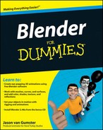
Your Blender screen should look something like the one in Figure 10-1.
Congratulations! You've just created your first animation in Blender. Here's what you've done: The largest part of the Ipo Curve Editor is a graph. Moving from left to right on this graph – its X-axis – is moving forward in time. Moving up and down on this graph changes the value of whatever channel you've selected from the list along the right side of the Ipo Curve Editor. So the curve that you created describes and controls the change in the cube's Z-axis location as you move forward in time. Blender creates the curve by interpolating between the control points you've created. You can see the result for yourself by playing back the animation. Keeping your mouse cursor in the Ipo Curve Editor window, press Alt+A. This makes a green vertical line move from left to right in the graph. As it does this, you should basically see your cube bouncing up and down in the 3D View. Press Esc to stop the playback. You can watch the animation in a more controlled way by left-clicking in the graph area of the Ipo Curve Editor and dragging your mouse cursor left and right. The vertical green line, called the timeline cursor, follows your mouse cursor, and you can watch the change happening in the 3D View. This is called scrubbing.
There's actually a screen layout in Blender specifically set up for animation. You can choose it from the Screen Layout button at the top of the Blender window or by using the Ctrl+left arrow hotkey combination. When you do this, you should have a screen layout that looks like the one in Figure 10-2.
This screen layout is pretty similar to the one you created in the earlier example, except that you also have an Outliner window and a Timeline window. The Outliner is helpful for selecting objects in complex scenes that have many, many objects to work with. The Timeline gives you a central place to control the playback of your overall animation. This way, you can use the Ipo Curve Editor to focus on specific detailed animations. Like the Ipo Curve Editor, you can scrub the Timeline by left-clicking in it and dragging your mouse cursor left and right.

Tip
One change I usually like to make to this layout is the addition of another 3D View window split from the Outliner. I set this window to a shaded or textured camera view and remove its header. I do this so that I can use any perspective in the main 3D View window but still retain an idea of what the camera sees. That way, I don't end up animating something that will never be on camera. In this camera-view window, I also disable the Transform Manipulator (Ctrl+Spacebar
Working in the Ipo Curve Editor is very similar to working in the 3D View. Middle-clicking moves around your view of the graph and Ctrl+middle-clicking allows you to interactively scale your view of the curve horizontally and vertically at the same time. If you prefer using your scroll wheel, you can navigate the entire graph that way. Plain scrolling zooms in and out, whereas Shift+scrolling moves the graph vertically and Ctrl+scrolling moves it vertically. You can select individual Ipo curves by right-clicking on them or toggle selecting all or no curves by pressing A. Even Border Select works by pressing B and using your mouse to draw a box around the curves you want to select.

You might be thinking, "Well, that was pretty neat, but there's got to be a more controlled way of adding control points than Ctrl+left-clicking in the Ipo Curve Editor. It seems awfully imprecise." And if you were thinking that, you'd be completely correct. Although it's possible to work like this, Blender uses a workflow that's a lot more like traditional hand-drawn animation. In traditional animation, a whole animated sequence is planned out ahead of time. Then an animator goes through and draws the primary poses of the character. These drawings are referred to as keyframes or keys. They're the poses that the character must make in order to most effectively convey the intended motion to the viewer. With the keys drawn, they are handed off to a second set of animators called the inbetweeners. These animators are responsible for drawing all of the frames between each of the keys in order to get smooth motion.
Translating this to how work is done in Blender, you should consider yourself the keyframe artist and Blender the inbetweener. Using the example at the beginning of this chapter, every time you Ctrl+left-clicked in the Ipo Curve Editor, you created a keyframe. By interpolating the curve between those keys, Blender creates the in-between frames. Some animation programs refer to this as tweening.
To have a workflow that's even more similar to traditional animation, you would prefer to be able to define your keyframes in the 3D View. Then you could use the Ipo Curve Editor to tweak the change from one keyframe to the next. And this is exactly what you can do. In the 3D View, press I to bring up the Insert Key menu, as shown in Figure 10-4.

Through this menu, you can create keyframes for the main animatable channels for an object. They are described in more detail here:
Loc: Insert a key for the object's X, Y, and Z location.
Rot: Insert a key for the object's rotation in the X, Y, and Z axes.
Scale: Insert a key for the object's scale in the X, Y, and Z axes.
LocRot/LocScale/LocRotScale/RotScale: Inserts keyframes for various combinations of the previous three values.
VisualLoc/VisualRot/VisualLocRot: Inserts keyframes for location, rotation, or both, but based on where the object is visually located in the scene. These options are explicitly made for use with constraints, which are covered later in this chapter.
Layer: Inserts a keyframe for the layers that the object exists on. Keyframing this channel is a great way to make objects disappear from view. Note that because layers are discrete elements and Blender can't smoothly transition from one to another, the curve for this channel jumps from one value to the next with no smooth interpolation.
Available: If you have already inserted keys for some of your object's channels, choosing this option adds a key for each of those already-existing curves in the Ipo Curve Editor. If there are no curves already created, no keyframes are inserted.
Mesh: This inserts a key for the mesh itself. This is important for shape keys, a topic covered in more detail in Chapter 11.
Note
When Blender sets keyframes for location, rotation, and scale, you should bear in mind which coordinate system the Ipo Curve Editor is using. Location is stored in global coordinates, whereas rotation and scale are stored in the object's local coordinate system.
So to see the basic workflow for animating in Blender, bring up the default scene (Ctrl+X) and use the following steps:
Switch to the Animation screen layout (Ctrl+left arrow).
Insert an initial location keyframe (I
This creates a keyframe at frame one in your animation. If you look at the Ipo Curve Editor, notice that LocX, LocY, and LocZ are highlighted and have colored blocks next to them.
Move forward ten frames (up arrow).
This puts you at frame eleven. The up arrow and down arrow hotkeys move you ten frames forward or backward in time, regardless of the window your mouse cursor is in. To move forward or back one frame at a time, use the left and right arrow keys. Of course, you could also use the Timeline or Ipo Curve Editor to change what frame you are in.
Grab your cube and move it to a different location in 3D space (G).
Insert a new location keyframe (I
Now you should have curves in the Ipo Curve Editor that describe the motion of the cube.
There is another way to insert keys, and it's actually a little bit easier. It's a feature called Autokey, and like its name indicates, it automatically creates keys when you move, resize, and scale your object. To enable the Autokey feature, look in the Timeline window. Next to the VCR-like controls for controlling animation playback is a button with a red circle on it, like the Record button on a VCR. Figure 10-5 shows this button. Left-click it to activate Autokey. Now you can simply use the Grab (G), Rotate (R), and Scale (S) tools as you move forward in time and keyframes are automatically inserted for you. Pretty sweet, huh?
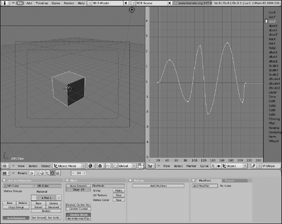
Some of the other Blender window types allow you to set keys for other attributes as well. For instance, if you bring up the Material buttons and press I with your mouse cursor in that window, a menu with a set of materials-related keyable channels appears. Figure 10-6 shows the different Insert Key menus that appear for the various Buttons windows.
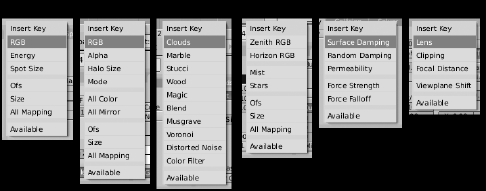
Figure 10-6. From L to R: Insert Key menus for Lamp, Material, Texture, World, and Physics, and the menu for Editing when a camera is selected.
You may notice that if you insert a key using these menus, many times, their curves don't seem to appear in the Ipo Curve Editor. This is because the types of keyable channels have been broken down and organized into seven different possible categories: Object, Material, World, Texture, Shape, Constraint, and Sequence. To show the curves and keyable channels in these categories, look in the Ipo Curve Editor's header. By default, you're looking at the Object curves, so there's a button in the header next to the Ipo datablock button that says Object. Left-click that button to see and choose from the other available Ipo types. Figure 10-7 shows what this menu looks like.
After you know how to add keyframes to your scene, the next logical thing to do is tweak, edit, and modify those keyframes as well as the interpolation between them. This, too, happens in the Ipo Curve Editor. Earlier in this chapter, I said the Ipo Curves Editor is similar to the 3D View and that individual motion curves could be selected by right-clicking or by using the B key for border selecting. Well, it goes further than that. Not only can you select motion curves in the Ipo Curve Editor, but you can Tab into Edit mode with them and edit them like a 2D Bézier curve object in the 3D View. The only constraint on this is that Ipo Curves cannot cross themselves. Having a curve that describes motion in time do a loopty-loop doesn't logically make any sense.
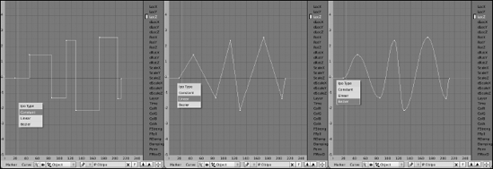
For more detailed descriptions of the hotkeys and controls for editing Bézier curves in Blender, have a look at Chapter 6. Selecting and moving control point handles, as well as the hotkeys for Free/Aligned (H), Auto (Shift+H), and Vector (V) handles all work as expected. However, because these curves are specially purposed for animation, you have a few additional controls over them. For instance, you can control the type of interpolation between control points on a selected curve by pressing T or going to Curve
Constant: This is sometimes called a step function because a series of them look like stair steps. Basically, this interpolation type keeps the value of one control point until it gets to the next one, where it instantly changes.
Linear: The interpolation from one control point to the next is a completely straight line. This is similar to changing both control points to have Vector handles.
Bézier: The default interpolation type. This uses Auto handles on the control points to smoothly transition from one to the next. In traditional animation, this is referred to easing in and easing out of a keyframe.
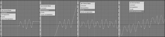
You can also change what a selected Ipo curve does before and after its first and last keyframes. This is called the curve's Extend Mode and you can change it by pressing E or navigating to Curve
Constant: This is the default setting. The values of the first and last control points are maintained into infinity beyond those points.
Extrapolation: Rather than maintaining the same value in perpetuity before and after the first and last control points, this extend mode takes the direction of the curve in those control points and extends the curve that way.
Cyclic: A Cyclic extend mode takes the entire shape of the curve from the first control point to the last one and repeats it before and after those "control points so that the same motion loops over and over forever.
Cyclic Extrapolation: This option combines the previous two extend modes. So the same motion loops before and after the first and last keyframes, but it loops in the direction that the Ipo curve is going when it gets to those points.
Figure 10-9 shows the menu for the different type of extend modes, as well as what each one looks like with a simple Ipo curve.
If you have an object with a high number of animation curves, it may be helpful to hide extraneous curves from view so you can focus on the ones you truly want to edit. To toggle a curve's visibility, Shift+left-click its name in the keyable channel list along the right side of the Ipo Curve Editor. Doing so shows its name in either white text or black text. Black text means the curve is hidden, whereas white text means it's visible. Also, if the channel has a color swatch to the left of it, then you know it's been keyed. That color swatch is useful for selecting the curve (left-click the swatch) as well as visually distinguishing one curve from another because the color in the swatch is the color of the curve in the graph of the Ipo Curve Editor.
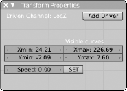
If you need explicit control over the placement of a curve or a control point, the Ipo Curve Editor has a floating panel like the 3D View has. You bring it up the same way too: either press N or choose View
There's another really helpful feature for editing curves in the Ipo Curve Editor. Often, you may run into the occasion where you need to edit all of the control points in a single keyframe to change the overall timing of your animation. It may be tempting to select all curves with the A key, Tab into Edit mode, and use Border Select (B) to select the strip of control points you want to move around. However, there's an cleaner and easier way to do this. Rather than go through that process, press K in the Ipo Curve Editor or choose View
Tip
When you're moving around keys or even control points in the Ipo Curve Editor, you should hold down Ctrl. This ensures that you've moving them around in frame-length increments. It's a good practice to make sure your keyframes actually happen on the frame, rather than between frames. If you're ever unsure as to whether a key is on the frame, select it (right-click) in the Ipo Curve Editor and press Shift+S
The Show Keys functionality also has one more trick up its sleeve. Move your mouse cursor into the 3D View and press K. Doing this actually shows ghosted wireframes of your object's keyframes. This is kind of a 3D version of something called onionskinning in traditional animation. This can give you a very clear picture of your entire animation at a glance. But wait, it gets better! Note that if you right-click one of the yellow key lines in the Ipo Curve Editor, the corresponding key is also highlighted in the 3D View. Now you can use your Grab (G), Rotate (R), and Scale (S) hotkeys to interactively edit and adjust that keyframe while the other keyframes are in view. How's that for totally awesome? Figure 10-11 shows the Show Keys feature in action.
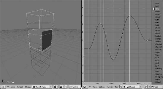
Figure 10-11. "Press K in the 3D View to show your object's keyframes and make them directly editable.
Table 10-1 covers some of the most common hotkeys and mouse actions used to control animation in the Ipo Curve Editor.
Table 10-1. Commonly Used Hotkeys and Mouse Actions for the Ipo Curve Editor
Mouse Action | Description | Hotkey | Description |
|---|---|---|---|
Left-click graph | Move time cursor | Alt+A | Playback animation |
Left-click channel | Hide/Reveal channel (Shift+left-click for multiple) | E | Extend Mode |
Left-click swatch | Select channel | K | Show keys |
Right-click | Select channel | O | Clean Ipo curves |
Middle-click | Pan graph | Shift+O | Smooth Ipo curves |
Ctrl+middle-click | Scale graph | N | Channel Properties |
Scroll | Zoom graph | Shift+S | Snap Menu |
Shift+scroll | Pan graph vertically | T | Ipo Type |
Ctrl+scroll | Pan graph horizontally | Home | Fit curves to graph |
Occasionally I get into conversations with people who assume that because there's a computer involved, doing good CG animation takes less time than traditional animation techniques. In most cases, this is not true. High quality work takes roughly the same amount of time, regardless of the technique. The time is just spent in different places. Whereas in traditional animation, a very large portion of the time is spent drawing the inbetween frames, CG animation lets the computer handle that. However, traditional animators don't have to worry as much about optimizing for render times, tweaking and re-tweaking simulated effects, or modeling, texturing, and rigging characters.
That said, computer animation does give you the opportunity to cut corners in places and make your life as an animator much simpler. One of the features that fits this description perfectly are constraints. Literally speaking, a constraint is a limitation put on one object by another, allowing the unconstrained object to control the behavior of the constrained one. The simplest example of a type of constraint is parenting. This is covered in more detail in Chapter 4, but as a quick example, bring up the default scene in Blender (Ctrl+X). Now Shift+right-click the Lamp so both it and the cube are selected and the Lamp is the active object. Press Ctrl+P
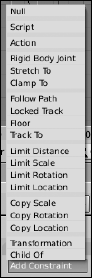
Although parenting with the Ctrl+P hotkey combination is a constraint in the literal since of the word, it's used in Blender for doing more things than simply binding the location, orientation, and size of one object to another. For that reason, it's not a constraint like the ones discussed later in this chapter. In fact, to see the actual constraints that you do have available to you, go to the Object buttons (F7) and left-click the Add Constraint button in the Constraints panel. When you do this, you see the menu that looks like the one in Figure 10-12.
Because of limitations to this book's page count, I can't cover the function of each and every constraint in full detail. However, the end of this chapter gives some usage examples for some of the more frequently used constraints.
Of all the different types of objects available to you in Blender, none of them are as useful or versatile in animation as the humble Empty. It's not much: just a little set of axes that indicate a position, orientation, and size in 3D space. It doesn't even show up when you render. However, this means that it's an ideal choice for use as control object and it's a phenomenal way to take advantage of constraints. To illustrate this, allow me to use simple parenting as an example again.
One of the things that 3D modelers like to have is a turnaround render of the model they create. Basically, it's like taking the model, placing it on a turntable, and spinning it in front of the camera. It's a great way to show off all sides of the model. Now, for simple models, you can just select the model, rotate it in the global Z-axis, and you're done. However, what if the model consists of many objects, or for some reason everything is at a strange angle that looks odd when spun around the Z-axis? Selecting and rotating all of those little objects can get time-consuming and annoying. A better way of handling it is with the following rig:
Add an Empty (spacebar
Grab the Empty and move it to somewhere at the center of the model (G).
Select the camera and position it so the model is in the center of view (right-click, G).
It would be wise to aim the camera roughly at the location of the Empty.
Add the Empty to your selection (Shift+right-click).
This makes the Empty the Active object in the selection.
Make the Empty the camera's parent (Ctrl+P
Select the Empty and insert a rotation keyframe (right-click, I
Rotate the Empty 90 degrees in the Z-axis and insert a new rotation keyframe (R
In doing this, you should notice that the camera obediently matches the Empty's rotation.
Bring up the Ipo Curve Editor and set the Extend Mode for the RotZ channel to Extrapolate (Shift+F6, right-click, E
Switch to the camera view and playback the animation (Numpad 0, Alt+A).
In the 3D View, you should be seeing what appears to be your model spinning in front of your camera. Congratulations, you've made a turnaround.
In this setup, the Empty behaves as the control for the camera. Imagine that there's a beam extending from the Empty's center to the camera's center and that rotating the Empty is the way to move that beam. And you can add to this. Suppose you wanted the Lamp to stay with the camera, rather than remaining static throughout the turnaround. You could solve this by parenting (Ctrl+P) the lamp to either the Empty or the Camera. Either way gets you the results you're looking for.
Using simple parenting is helpful in quite a few instances, but it's often not as flexible as you need it to be. You can't control or animate the parenting influence or just use the parent object's rotation without inheriting the location and scale as well. And you can't have movement of the parent object in the global X-axis influence the child's local X-axis location. More often than not, you need these sorts of refined controls rather than the somewhat ham-fisted Ctrl+P parenting.
To this end, there are a set of constraints that provide you with just this sort of control. They are the Copy Location, Copy Rotation, and Copy Scale constraints. Figure 10-13 shows what each of these constraints look like when added in the Constraints panel.
Tip
You can mix and match multiple constraints on a single object in a way that's very similar to the way you can add multiple modifiers to an object. So if you need both a Copy Location and a Copy Rotation constraint, just add both. After you add them, you can change which order they come in the stack to make sure they suit your needs.

Tip
Words and picture aren't always the best way of explaining how constraints work. It's often more to your benefit to see them in action. To that end, CD-ROM that accompanies this book has a few example files that illustrate how these constraints work. It's worth it to load them up in Blender and play with them to really get a good sense for how these very powerful tools work.
Probably the most apparent thing about these constraints is how similar their options are to one another. The most critical setting, however, is the object that you name in the Target field. If you're using an Empty as your control object, this is where you type that Empty's name. Unless you do so, the Constraint Name field at the top of the constraint block remains bright red and the constraint simply won't work.
Next up is the Offset button. This is useful if you've already adjusted your object's location, rotation, or scale prior to adding the constraint. By default, this feature is off, so the constrained object mirrors the target object's behavior completely and exactly. With it enabled, though, the object adds the target object's transformation to the constrained object's already set location, rotation, or scale values. The best way to see this is to create a Copy Location constraint with the following steps:
Start with the default scene (Ctrl+X).
Grab the default cube to a different location (G).
Add an Empty (spacebar
Select the cube and put a Copy Location constraint on it (right-click, F7
When you do this, the cube automatically snaps directly to the Empty's location.
Left-click the Offset button in the Constraints panel.
The cube goes back to its original position. Grabbing (G) the Empty influences the cube's location from there.
To the right of the Offset button are a series of six buttons, with the X, Y, and Z buttons already enabled, separated by disabled buttons with minus signs on them. These buttons control which axis or axes the target object influences. If the axis button is enabled and the minus button next to it is also enabled, the target object has an inverted influence on the constrained object in that axis. Using the previous Copy Location example, if you left-click the X button and then Grab the Empty and move it in the X-axis (G
Beyond these options, one of the most useful settings that's available to all constraints is at the bottom of each constraint block. I'm talking about the Influence slider. This slider works on a scale from zero to one, with zero being the least amount of influence and one being the largest amount. With this, you have the capability of just partially copying the target object's attributes. There's more to it, though. Notice the Show and Key buttons to the right of the slider. With the Key button, you can animate the influence of the constraint. The show button makes the constraint curves visible in an Ipo Curve Editor window if you have one open. Say you're working on an animation that involves a character with telekinetic powers using his ability to make a ball fly to his hand. You can do that by animating the influence of a Copy Location constraint on the ball. The character's hand is the target and you start with zero influence. Then, when you want the ball to fly to his hand, you increase the influence to one and set a new keyframe. BAM! Telekinetic character!
Note
When setting keys for constraints, the Ipo curves for the influence doesn't show up in the default Ipo Curve Editor. To see these curves, either press the Show button next to the Influence slider or use the Ipo Type menu in the Ipo Curve Editor's header.
Tip
It's in your best interest to use the Show button to see the constraint Ipo. The reason for this is that if there are multiple animated constraints on the same object, left-clicking Show insures that you're looking at the right one.
The CSpace buttons in these constraints are pretty interesting, although they have a somewhat specialized use. Specifically speaking, they only really have any effect if the constrained object is also parented to an object that is not the target object. Consider the previous offset Copy Location example, but make a few changes:
Rotate the target Empty an arbitrary amount in the Z-axis (R
Somewhere around 30 degrees should be fine — just enough so that it's different from the global coordinate system.
Add a new Empty to the scene (spacebar
Grab the new Empty and move it so that it's not near the origin (G).
If you want some specific numbers, bring up the Transform Properties floating panel and set LocX to −2, LocY to 2, and LocZ to 7.
Rotate the new Empty some arbitrary amount in the Z-axis (R
Again, no specific number is necessary — just something that offsets it from the global coordinate space.
Parent the cube to the new Empty (right-click the cube, Shift+right-click the new Empty, Ctrl+P
Now with the above set up, you can play with the CSpace options. The left button controls the coordinate space in which the constraint evaluates the target and the right button controls the coordinate space in which the constraint evaluates the constrained, or owner, object. With both of these values set to World Space, the constraint behaves as you would expect. Move the target Empty and the cube obediently follows along. However, left-click the right button and change the Owner Space to Local (Without Parent) Space. Now, select the target Empty and move it in the global X-axis (right-click, G
Okay, so I lied a little bit when I said you couldn't control or animate the influence of a parent-child relationship in Blender. That was a half-truth. It's true that if you use Ctrl+P to make one object the parent of another, no additional controls are available to you. However, if you add a Child Of constraint, the situation changes a bit. Figure 10-14 shows that if you create a parent-child relationship between objects using this constraint, you have quite a few controls available to you.

After you type in the name of the object you wish to use as the parent, you can choose any combination of location, rotation, and scale channels in the X, Y, and Z axes for the parent relationship. You can even take advantage of having an offset from where the standard parent-child relationship would put your object. And, like the other constraints, you can control and animate how much this constraint has an effect on your object by using the Influence slider and keying its values over time.
Another unique feature of this constraint is the VG field that shows up after you type in a valid object in the OB field. In the VG field, you can type the name of a vertex group in the parent mesh. When you do this, the constrained child object is the child of those specific vertices. To create a vertex group, tab into Edit mode on the parent object and select a couple of vertices. Then switch to the Editing buttons (F9) and left-click the New button under Vertex Groups in the Link and Materials button. This creates a new vertex group called Group. To make the vertices you've selected part of the group, left-click the Assign button. This is covered in more detail in Chapter 11. Figure 10-15 shows a Suzanne head parented to a vertex group consisting of a single vertex on a circle mesh.
In many ways, this constraint is a much more flexible and powerful way of parenting than using Ctrl+P. Of course, regular parenting can do some things that this constraint can't, like Dupliverts. Perhaps, however, future versions of Blender will merge the functions of these two features.

Often when animating objects, it's helpful to prevent objects from being moved, rotated, or scaled beyond a certain extent. Say you're animating a character trapped inside a glass dome. It would be helpful to you as an animator if Blender forced you to keep that character within that space. Sure you could just pay attention to where your character is and visually make sure he doesn't accidentally go farther than he should be allowed, but why do the extra work if you can have Blender do it for you? Figure 10-16 shows the constraint options for most of the limiting constraints Blender offers you.

Descriptions of what each of these constraints does are below:
Limit Location/Rotation/Scale: Unlike most of the other constraints, these three constraints don't have a target object that they're constrained to. They're just limitations on what the object can do within its own space. For any of them, you can define minimum and maximum limits in the X, Y, and Z axes. After you've defined the limit, you enable it by left-clicking the button for that limit next to it. The For Transform button that's in each of these constraints can be pretty helpful. To better understand what it does, enable the Transform Properties floating panel in the 3D View. If you have limits and For Transform is not enabled, the values in the Transform Properties panel change even after you reach the limits defined by the constraint. However, if you enable For Transform, the value in the Transform Properties panel is clipped to the limitations you defined with the constraint.
Limit Distance: This constraint is similar to the previous ones except it relates to the distance from the centerpoint of a target object. The Clamp Region menu gives you three ways to use this distance:
Inside: The constrained object can only move in the sphere of space defined by the Distance value.
Outside: The constrained object can never enter the sphere of space defined by the Distance value.
Surface: The constrained object is always the same distance from the target object, no more and no less.
Floor: The Floor constraint uses the centerpoint of a target object to define a plane that the centerpoint of the constrained object can't move beyond. So, technically, you can use this constraint to define more than a floor; you can also use it to define walls and a ceiling as well. One thing to keep in mind is that this constraint defines a plane. If your target object is an uneven surface, it will not use that object's geometry to define the limit of the constrained object, just it's centerpoint. Despite this limitation, this constraint is actually quite useful. This is especially true if you enable the Use Rot button. Doing that allows the constrained object to recognize the rotation of the target object, so you can have an inclined floor if you like.
Tip
When animating while using constraints, particularly limiting constraints, it's in your best interest to insert keyframes using the VisualLoc and VisualRot. This sets the keyframe to where the object is located visually, within the limits of the constraint, rather than how you actually transformed the object. For instance, assume you have a Floor constraint on an object that you're animating to fall from some height and land on a floor plane that's even with the XY grid. For the landing, you Grab (G) object and move your mouse cursor 4 Blender units below the XY grid. Of course, because of the constraint, your object stops following the mouse when it hits the floor. Now, if you insert a regular Loc keyframe here, the Z-axis location of the object is set to −4.0 even though the object can't go below zero. However, if you insert a VisualLoc key, the object's Z-axis location is set to what you see it as, zero.
Another set of constraints that are helpful for animation are tracking constraints. Their basic purpose is to make the constrained object point either directly at or in the general direction of the target object. They're useful for things like controlling the eye movement of characters or building mechanical rigs like pistons. Figure 10-17 shows the options for three of Blender's tracking constraints.
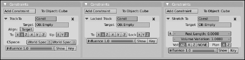
Descriptions of each of these constraints are below:
Track To: Of these constraints, this one is the most straightforward. In other programs, this constraint may be referred to as the Look At constraint, and that's what it does. It forces the constrained object to point at the target object. The best way to see this would be to load the default scene (Ctrl+X) and add a Track To constraint to the camera with the target object being the cube. Now, no matter where you move the camera to, it always points at the cube's centerpoint. By left-clicking the X, Y, and Z buttons next to the To and Up labels, you can control how the constrained object points to the target.
Locked Track: The Locked Track constraint is similar to the Track To constraint, with one large exception: It only allows the constrained object to rotate on a single axis. This means that the constrained object points in the general direction of the target, but not necessarily directly at it. A good way to think about this is to imagine you're wearing a neck brace. With the brace on, you can't look up or down; you can only rotate your head left and right. So if a bird flies overhead, you can't look up to see it pass. All you can do is turn around and hope to see the bird flying away.
Stretch To: This constraint isn't exactly a tracking constraint like Track To and Locked Track, but it's behavior is similar. It makes the constrained object point toward the target object like the Track To constraint. However, it also changes the constrained objects scale relative to the distance that the target is away from it, stretching that object toward the target. And it can even try to preserve the volume of the constrained object to make it seem like it's really stretching. This is a great constraint for cartoony effects as well as controlling organic deformations such as rubber balls and the human tongue. On a complex character rig, you can use the Stretch To constraint to help simulate muscle bulging.