
Chapter 3
The Fundamental Drivers of Asset Class Returns
Ray Dalio took his understanding of the relationships that exist between economic and market shifts to create a revolutionary new and better way to structure a portfolio. He called it All Weather because it is designed to perform well across economic environments. Those investment firms that adopted the concepts (and could not use the All Weather name because it was Bridgewater's) call their products risk parity. Regardless of what we call it, it is a simple and effective way to balance your portfolio so that it lowers risk without lowering returns, and I want you to understand it. It is an elegantly simple solution to an important problem.
My goal in this book is to describe this framework for building a mix of asset classes that can reasonably be expected to deliver stable returns through time. Volatility is obviously unavoidable, but an asset allocation that has a decent probability of experiencing an extended period of significant underperformance is unacceptable. A necessary prerequisite to constructing such an efficient allocation is an understanding of the key fundamental drivers that result in the returns that you see. A better appreciation of the source of asset class returns will provide the needed insight for assembling an optimal asset allocation and minimizing volatility over time. If you understand the source of returns and what factors make them volatile, you will be better positioned to appreciate how to neutralize the risk as much as possible. In this chapter I share with you a very effective methodology that I learned from Bridgewater.
The fundamental reasons asset class returns are volatile can be classified into three broad categories: (1) shifts in the economic environment, (2) shifts in risk appetite, and (3) shifts in expectations of future cash rates. The latter two sources of volatility are unavoidable if you invest in risky asset classes. These risks are inherent and necessary. You can understand them, but you can't do much to protect yourself against these two factors. Fortunately, these two infrequently result in big losses in asset class returns, and the pain generally only lasts for a short time when losses do occur. The first risk—shifts in the economic environment—that impacts returns occurs all the time and can persist for long stretches. The good news is this risk is diversifiable. That is, you have the opportunity to build an appropriately balanced asset allocation that is targeted to minimize the volatility associated with this risk. That, in a sense, is the entire purpose of this book: to introduce you to a methodology to balance your portfolio by diversifying against the risk that is diversifiable.
Although you can't protect yourself against all three risks, it is crucial to appreciate where they all come from. A comprehensive understanding of the fundamental drivers of asset class returns will help establish context for the discussion that follows in later chapters. Furthermore, the insight will better prepare you for actual experience. The dominant source of volatility in asset class returns—shifting economic climates—can largely be neutralized with the methodology introduced in this book. That still leaves the other two that will inevitably cause a well-balanced portfolio to still experience some volatility and losses over shorter time frames. By understanding the core causes of this volatility in advance and by being equipped to explain why returns fluctuate, you are more likely to make prudent investment choices during challenging periods. For this reason, this chapter will begin by breaking down asset class returns into their core components.
Breaking Down Returns into Cash Plus Excess Return
The first step in isolating the underlying source of volatility is to break down the return of an asset class into its two most basic components. Previously I mentioned three key sources of returns and volatility. Before discussing these factors in more detail, I would like to begin at an even more basic level.
The return of any asset class can be broken down into two parts:
- The return of cash
- The excess return above cash
Why is this? When you make an investment you are effectively exchanging cash for an asset with the objective of exchanging it back for cash at some point in the future (because you can only spend cash). For you to make this exchange requires that the asset offer an expected return above the rate for cash to adequately compensate you for taking the risk of loss with your money. Another way to think of this is any asset class (such as stocks, bonds, commodities, real estate, etc.) offers a return that is cash plus some excess return. This excess return above cash is often termed the risk premium. It is the premium you receive for taking risk.
In fact, the excess return above cash you receive for taking risk is the return that really matters. For example, if stocks earned 10 percent per year for 10 years, but cash earned 8 percent per year during the same time frame, then it is the 2 percent excess return above cash that is significant. You could have earned 8 percent without taking any risk, which makes the 10 percent stock return much less impressive. Conversely, if cash had only earned 1 percent per annum during that time, then the 10 percent stock return becomes more meaningful. For this simple reason, most of the focus in this book will be on the excess returns above cash rather than total returns (which includes the embedded cash return). Most investors mistakenly overemphasize total returns in their analysis and therefore fail to appropriately break down returns into their fundamental components.
To summarize, the total return of an asset class is merely the sum of its core parts:
Looking at these two parts separately will reveal some interesting facts about the true source of risk in asset class returns. The return of cash has very low volatility. However, the excess return above cash is highly volatile and therefore explains nearly all the volatility that is embedded in asset class total returns. Excess returns above cash can be further subdivided into three components. It is these three fundamental drivers of asset class returns that explain why asset classes are volatile.
I will begin with a detailed walkthrough on the return of cash, followed by a deep dive into excess returns above cash. The final section of the chapter will bring the two together to leave you with a good understanding of the main drivers of asset class returns and the key implications for prudent portfolio construction. The main idea here is to get you to start thinking about where returns come from and why they fluctuate. This core understanding will set the foundation for a new way to think about the entire asset allocation construction process. With a fresh perspective, the methodology for building a well-balanced portfolio should make more sense.
The Return of Cash
The simplest asset to understand is cash. Cash earns an interest rate that is, by and large, set by the Fed. The first chapter explained that the Fed controls this rate and adjusts the levels to help stabilize the economy. When growth or inflation is too strong, the Fed raises the rate to slow an overheated economy and get it back on a more sustainable track. When growth or inflation is too weak, then the Fed takes the opposite approach by lowering rates to stimulate more borrowing to help engineer a rebound. These conditions normally do not change rapidly and instead gradually shift over time. Consequently, the return of cash is predictably constant during most environments. Wild swings in the rate of cash would result in significant volatility in the economic environment. Since the Fed is commonsensically trying to maintain economic stability, it is incented to keep cash rates as steady as possible.
As a result, the interest rate for cash is fairly stable nearly all the time. If the Fed sets short-term rates at 5 percent, then you earn about 5 percent per year on your cash. This investment is the safest way to earn a return on your money. There is essentially no risk of loss, and as a result the cash rate is widely considered to be the risk-free rate. The only volatility you will experience is the change in the interest rate. It could be 15 or 5 or even 0 percent. However, it has never been negative in absolute terms (although it can be negative in real terms, meaning that the interest rate may be less than the rate of inflation).
Figure 3.1 displays the average return of cash over every 10-year period since 1927. Ten-year average rolling returns are used to smooth out shorter-term fluctuations and to demonstrate that over a long time period, cash returns have been extremely reliable. The average return of cash since 1927 has been 3.8 percent per year. You will notice that over every 10-year period the return of cash has, by and large, not materially fluctuated from its long-term average, and it has never been negative. This is exactly why cash is considered the risk-free asset.

Figure 3.1 10-Year Rolling Cash Returns
Source: Bloomberg and Bridgewater.
Excess Returns above Cash
You may not be satisfied with just holding cash. The rate may be too low or you may simply wish to try to achieve higher returns by increasing the risk that you take. If you want to take more risk, then you can do so by investing in other asset classes (such as stocks, bonds, commodities, and so on). By risk, I am referring both to the risk of loss of capital and the volatility of returns. The more volatile the returns of an investment are, the greater the risk of losing money. This is true because the return may be negative when you sell. The higher the volatility, the greater is the likelihood that you could earn a return less than cash offers (which, again, is the return you would have had without taking any risk). Generally speaking, the more risk you take, the higher the expected return. This relationship should hold over time; otherwise investors would not be willing to take the added risk. Note that this does not mean that you will automatically earn higher returns simply by taking more risk. If returns were guaranteed, then these investments would not be risky. This highlights a very common, unwarranted assumption and oversight. More risk means the expected return is higher, but the actual results may be lower. The key insight to appreciate is what may cause the actual results to fall below the expected returns. If you can understand the causes, then you will be more fully informed to protect yourself against the impact of some of these occurrences.
Different asset classes offer various excess returns above cash. The goal is to capture these excess returns over time and to do so with as little risk as possible. The problem is that the excess returns fluctuate over time and are not stable like cash. The excess returns are roughly commensurate with the level of risk taken. The higher the level of risk, the higher the expected excess return will be. This relationship makes sense because if it were not true, then investors would choose to take less risk for a similar expected excess return. Stocks are riskier than bonds and therefore enjoy higher expected excess returns over time. Long-term historical excess returns support this assumption.
Since 1927, the four asset classes on which I will focus—stocks, long-term Treasury bonds, long-term Treasury Inflation-Protected Securities (TIPS), and commodities—have provided excess returns above cash, as listed in Table 3.1.
Table 3.1 Average Excess Returns for Four Asset Classes (1927–2013)
| Asset Class | Average Excess Return |
| Equities | 5.6% |
| Long-Term Treasuries | 1.4% |
| Long-Term TIPS | 4.6% |
| Commodities | 2.0% |
Source: Throughout this book the following indexes were used to calculate returns for the various asset classes:
U.S. equities: S&P 500 Index. Data provided by Bloomberg.
Long-term Treasuries: constant 30-year maturity Treasury index. Data provided by Bloomberg and Bridgewater Associates.
Core bonds (for the bond component of the 60/40 portfolio): 1976–2013 Barclays U.S. Aggregate Bond Index. 1927–1975 U.S. Treasury constant 10-year maturity index. Data provided by Bloomberg and Bridgewater.
Commodities: 1970–2013 Goldman Sachs Commodity Index. 1934–1969 Dow Jones Futures Index. 1927–1933 Reuters/Jeffries-CRB Total Return Index. Data provided by Bloomberg and Bridgewater.
Long-term TIPS: 1997–2013 constant 20-year duration US TIPS index. For periods prior to TIPS inception in 1997, Bridgewater simulated TIPS returns using actual Treasury returns, actual inflation rates, and Bridgewater's proprietary methodology.
These figures represent average excess returns over 86 years. (I am able to show TIPS returns since 1927, even though TIPS were created in 1997, by using Bridgewater's data that is based on their proprietary methodology to simulate a long-term historical return series. See also the explanation accompanying Table 6.1 in Chapter 6.) During this time, significant volatility in returns was experienced. One way to observe the volatility in historical returns is to analyze excess returns above cash over longer time frames. A long time horizon may consist of 10 years (and probably even shorter than that for most investors). A helpful way to see the volatility that comes from investing in these asset classes is to strip out the relatively stable return of cash and isolate the volatility in excess returns above cash. This is the volatility that is associated with unexpected shifts in the three key sources of returns that will be covered in this chapter. Figures 3.2a–3.2d show the rolling 10-year historical excess returns above cash for the four asset classes.

Figure 3.2a 10-Year Rolling Equity Excess Returns

Figure 3.2b 10-Year Rolling Long-Term Treasuries Excess Returns

Figure 3.2c 10-Year Rolling Long-Term TIPS Excess Returns

Figure 3.2d 10-Year Rolling Commodities Excess Returns
Notice how volatile the excess returns of each individual asset class have been when compared to their average excess returns. Most asset classes rarely returned the average even over a 10-year period, which is a long time for most investors. You are more likely to earn a return either far above or far below the average long-term expected return—even over a long time frame (such as 10 years)—when investing in any individual asset class. Other asset classes are similarly volatile. The key insight is that the excess returns above cash can be far above and far below the average for long periods of time.
What causes this volatility? There are three ways to separate the fundamental drivers of excess returns above cash. Two are nondiversifiable; the other can be mostly neutralized and is therefore the main subject of this book. The following three key factors impact the excess returns above cash:
- Shifts in the economic environment (unexpected changes in growth and inflation). This risk is diversifiable.
- Shifts in risk appetite, or the general market willingness to take risk. This risk is not diversifiable.
- Shifts in expectations of future cash rates. This risk is not diversifiable.
Shifts in the Economic Environment (a Risk You Can Diversify Against)
It is important to understand what you are really doing when you exchange cash for an asset class. This trade is largely a bet on shifts in the future economic environment. I am referring to changes in economic growth and inflation when describing the overall economic climate. In the first chapter I emphasized that the Fed tries to minimize the volatility of the economy in terms of growth and inflation by controlling interest rates and printing money, as necessitated by prevailing conditions. These are also the key forces that impact asset class returns because they are fundamental to what makes an investment.
When you decide to convert your safe cash into an asset class, you do so with the expectation that at some point in the future you will be able to convert it back to cash at a profit. If you did not expect this, then you would not accept the risk of losing money. More precisely, you convert cash into another asset with some expectation about the future economic climate. You have this expectation because in order to profit from the exchange, you factor in what future growth and inflation will be. Your expectation of inflation matters because you want to be compensated in real terms for the risk that you are taking. You need the return achieved from taking risk to exceed the rate of inflation in order for you to improve your purchasing power. After all, you can only spend cash, and the main reason you exchange cash for another asset class is because you expect to improve your purchasing power in the future. Thus, your expectation about the rate of inflation—or general increase in future prices of goods and services—is a critical factor.
Economic growth also influences your decision. If you anticipate strong economic growth, then you would be willing to accept a smaller piece of the future (if you are buying equities) or ask for a higher yield (if you are buying bonds), all else being equal. If you feel that growth is going to be very weak, then you would demand a bigger cushion in the price paid for equities in order to give you added protection. In this scenario you would be willing to accept a lower yield from bonds because of the safety it provides.
In diving a little deeper into why it is that changes in the economic environment impact asset class returns, I will use examples that feature the two most familiar asset classes, bonds and stocks.
Bonds: Why Shifts in the Economic Environment Impact Returns
If I exchange my cash for an investment in U.S. government-guaranteed Treasury bonds, then I am in effect making a bet that I will earn more with this investment than I would by simply holding cash over the same time frame. Since Treasury bonds held to maturity have very little risk of loss due to credit impairment, they are effectively a longer-duration version of the risk-free cash rate. I have a choice of low-risk investments: (1) hold cash and earn the variable interest rate over time, or (2) lock in a fixed rate by investing in a bond and take the risk that I would have done better holding cash. You make a similar decision when you are deciding on a home loan. You would select a variable rate loan if you wanted to take the risk that short-term rates will average less than the fixed rate you can guarantee today. In the case of buying a bond, you essentially are taking the other side of the transaction. Instead of being the borrower you become the lender, and the choice between a fixed or floating rate is a similar decision and is based on your expectation of future cash rates.
The key insight is to appreciate what would cause cash rates to shift over time. Changes in economic growth and inflation result in a reaction by the Fed to adjust interest rates (as was discussed in the first chapter). Thus, the price of the Treasury bond will change between now and maturity based on what transpires in the economic environment relative to what was expected at the time you purchased the bond. As the Fed lowers rates in response to falling growth or weak inflation, then the price of the bond rises. More precisely, what really matters is how cash rates shift relative to the path that was reflected in the price when you bought the bond. If cash is yielding 3 percent and the bond 6 percent, then rising interest rates are already discounted in the price. The fact that they rise is not necessarily a negative for the price of your bond because that eventuality was already factored in the price. That is exactly why you got 6 percent instead of 3 percent for your investment. The key is how the future path of cash varies relative to the path that had been priced in at the time you made your initial investment, which was based on a certain expectation of future growth and inflation outcomes.
Stocks: Why Shifts in the Economic Environment Impact Returns
I now turn to another example of the same dynamic to further clarify why shifts in the economic environment affect asset class returns. When you decide to invest in a broad portfolio of stocks, you are also making a statement about future economic growth and inflation. If you get 5 percent per year economic growth over time and the market was only pricing in 2 percent growth, then you are likely to do well with your stock investment. Companies generally earn more money when the economy is growing faster, and when they earn more the performance for shareholders normally improves. That is, you might expect higher than the average excess return during these periods. Logically, the opposite also holds true. If the market discounts 5 percent growth and only 1 percent growth actually transpires, then there is a good chance that stocks will underperform their average return as companies earn less than expected.
Likewise, shifts in inflation impact returns. Rising costs negatively affect stock prices because of the inability to pass on the entire cost increase to customers, resulting in lower profits. Again, this is all versus what was expected at the time the price was set. If high inflation was already priced in and we experience low inflation, then that is a huge positive for stock prices. Putting shifts in inflation and growth together and how both relate to prior expectations will provide you with a better sense of the key drivers of returns over time.
Perhaps a helpful way to better appreciate the impact of shifts in the economic environment on the returns of stocks is to review U.S. stock market history. I will begin with a memorable time period for many of today's investors. The greatest bull market in the history of U.S. stocks took place from 1982 to 1999. The market averaged about 13 percent excess returns per year during that stretch (cash also earned about 5 percent per year for a total return of around 18 percent per year!). It was an age in which vast fortunes were created. The unforgettable events that defined this extraordinary run included the curbing of the runaway inflation that had plagued the nation the previous decade, interest rates that fell from the highest levels in history, sustained economic growth for nearly two decades and, to top it all, an Internet bubble that far exceeded expectations.
The more precise reason the stock market performed so well was because the U.S. economy grew faster than most people had expected, and inflation declined much more than anticipated. In short, investors were expecting a much worse economic scenario than what actually transpired. Given these sets of conditions, which represent the ultimate tailwind for equities, it should be no surprise that stocks fared so well.
The previous two decades had effectively set the stage for the success of the 1980s and 1990s. A completely different experience plagued investors from 1963 to 1981. During this 18-year phase the United States suffered through the worst increase in inflation in its history. Interest rates rose more than ever before (surging from 4 percent to 15 percent) and inflation peaked at nearly 15 percent. All of this occurred concurrently with slower than discounted growth. The economic scenario of high inflation and low growth tends to be a terrible backdrop for equities. Predictably, risky stocks earned the same return as risk-free cash for over 18 years! Imagine the investors who had bought stocks for the long run, lived through all the ups and downs of the 1960s and 1970s, and had nothing to show for it. Certainly such an experience would dampen future expectations. Such widespread pessimism was captured on the cover of BusinessWeek in 1979 as it infamously proclaimed “The Death of Equities.” Of course, these low expectations sowed the seeds for the great run during the aforementioned 1980s and 1990s.
The stagflation (a period of high inflation and weak growth) of the 1970s was nothing when compared to the devastation that had roiled the economy and markets several decades earlier. From 1929 to 1949, the U.S. economy suffered through one of its worst periods in history. These 20 years were characterized by a major depression and deflation—a completely different set of conditions when compared to the 1982 to 1999 environment. Thus, stocks performed dreadfully as should be anticipated given these difficult conditions. During one 33-month run the stock market fell 84 percent! Those who lived through the Great Depression and much of the 1930s and 1940s never were the same again. The horrors of the severe market and economic downturn had scarred them for life.
Sadly, the recent environment from 2000 to 2013 is not much different from the experience of the 1930s and 1940s. Growth severely underperformed expectations and has caused equities to do much worse than many had thought possible 13 years earlier. The past decade included two periods in which the value of the stock market fell by half (2000–2002 and 2008–2009). The bursting of the Internet bubble, an extraordinary housing collapse, and the 2008 credit crisis that pushed the economy to the brink of another great depression caused devastating market downturns. Consequently, stocks barely outperformed cash for the first 13 years of the new century, a reality that extremely few market experts had predicted at the height of the Internet bubble.
The lesson from these historical experiences is clear: The economic environment by and large drives the returns of stocks. The market outperforms during better times and underperforms during periods dominated by weaker economic conditions. More succinctly, when growth outpaces market expectations and when inflation comes in lower than discounted, the stage has been set for significant upside in equities and vice versa.
All Asset Classes: Why Shifts in the Economic Environment Impact Returns
The same logic that applies to stocks holds true for every asset class. Each market segment, whether we are talking about stocks, bonds, commodities, inflation-hedged assets, or just about any other asset contains inherent biases to various economic environments. Rising growth tends to be favorable for stocks and commodities, whereas falling growth is generally better for bonds. Rising inflation benefits inflation-hedged assets like TIPS and commodities, just as falling inflation helps stocks and traditional bonds. Much greater detail about the impact of the economic environment on these asset classes and others will be provided in later chapters. For now, you should appreciate that each asset class is simply a package of changes in the future economic environment and a risk premium level above cash.
Importantly, the reason that the risk of changes in the economic environment can be neutralized is logical and intuitive. This source of risk does not impact every asset class similarly. The impact is simultaneous, but each asset class has different inherent biases to each economic environment, so the resulting returns may be positive or negative. One particular economic climate may be negative for one asset class and simultaneously positive for another due to a perfectly reasonable and predictable explanation.
The critical insight here is that there always will be the risk that the economic environment will drastically and unexpectedly change. However, the key distinction between shifts in the economic environment and the other two risks—shifts in risk appetite and shifts in expectations of future cash rates—is the impact of shifts in the economic environment is different toward various asset classes. Moreover, these relationships, as will be discussed later, are highly reliable and logical. That is, while the outcome is always uncertain, the cause-effect relationships between shifts in the economic environment and various asset class returns are far more predictable. You don't have to know what the future holds, but you should know how different asset classes will react to different economic conditions. And it is the reliability in the relationships that provides the opportunity to diversify against the risk of adverse economic outcomes.
Shifts in Risk Appetite (Not a Diversifiable Risk)
Shifting risk appetite represents the second fundamental driver of excess returns. Think of risk appetite as the amount of excess return above cash you would be willing to accept to take the risk of investing your cash in asset classes. If you are feeling optimistic and your animal spirits are stirring, then you may be willing to accept a lower expected return for a certain level of risk than during more normal times. Alternatively, if you are really concerned about the future and think we may be headed for challenging and uncertain times, then you may require a higher expected return to part with your cash. The fact that you may demand a different level of excess return above cash depending on the environment should sound intuitive. Imagine if I approached you at the depths of the 2008 crisis and asked you to invest in my company at a price that offered a return of 4 percent above cash over time. Compare that to considering the same offer in the early 1990s as the momentum of strong economic growth was in its early stages. You would certainly reject my proposal in the first case and may seriously consider accepting it in the second. After all, both offers come with uncertainty, but you may reasonably conclude that the first has much greater downside risk. Your general fear about the uncertainty in the global economy would likely cause you to demand a higher excess return to part with your safe cash.
You are only one investor; however, the truth is that the majority of market participants use the same logic that supports your instinct in this example (probably more so than you realize). And it is the majority that sets the consensus view, which in turn establishes the market price. The consensus, by definition, is the market. The pendulum swings to extremes over time. When the majority is fearful, the demand for higher excess returns dominates, and when it is popular to be more aggressive, then lower expected excess returns exist. Fear and greed are another way to view these changes. At times, we are greedy for a higher return than cash offers and are willing to accept less for the same amount of risk. At other points in time we are fearful of losses and will only take risk if outsized returns are offered. Interestingly, greed often follows good periods and fear comes after severe downturns. That is, emotion tends to be a reactive rather than a proactive phenomenon.
How do changes in risk appetite affect prices and returns? What does it mean when the appetite for risk goes up or down? In simple terms, your return for an investment is the price you get when you sell (Y) minus the price you paid when you bought (X). The higher price X is, the lower your return, all else being equal, because of the less attractive entry point. When the appetite for risk declines, then the price falls to compensate you for taking risk. The lower the current price, the higher the potential forward-looking return if you buy. This is how shifts in risk appetite add to volatility in asset class prices.
The impact to asset classes is most visible during extreme periods. You may know that there exist rare environments when investors are terrified of taking any risk and sell all risky asset classes in favor of cash. Two stark examples of this environment include the Great Depression and the 2008–2009 crisis. During those two periods the markets were characterized by fear and the focus shifted to return of capital rather than return on capital. There was no desire to lend during these climates, so there was little access to credit. Forced sales of assets and heightened demand for cash caused risk premiums of all risky asset classes to concurrently skyrocket.
These severe cases help demonstrate why shifts in risk premiums, or risk appetite, are not diversifiable risks. As an investor in asset classes, this is a risk you are constantly subject to and there is no way to minimize it. Shifts in risk appetite understandably and simultaneously impact all asset classes. Therefore, there is no magic combination of asset classes that will help insulate you, since they are all affected in the same direction. That is, all asset classes are negatively impacted as risk appetite falls and risk premiums rise (or positively impacted as risk appetite rises and risk premiums fall).
The final important point about shifting risk appetite is the difficulty in avoiding this risk entirely. You might argue that investors can simply own cash when risk premiums are low and wait for risk premiums to rise before reallocating into riskier asset classes. However, you should keep in mind that your future appetite for risk is highly dependent on the state of the economy, your personal financial situation, the general momentum at the time, and many other factors. Most of these important inputs cannot be known because they have yet to occur. You don't even know how you are going to feel in the future, so how can you presume to know the collective mind-set of everyone else?
Shifts in Expectations of Future Cash Rates (Not a Diversifiable Risk)
The third and final fundamental driver of excess returns is shifts in expectations of future cash rates. Earlier I explained that the rate of cash is relatively stable. The steadiness of cash returns can, however, be misleading. Although current cash rates are not highly volatile, shifts in expectations of future cash rates contribute to volatility of asset class excess returns. The reason this is true is related to a central theme that will be repeated throughout this book. With any return series, what really matters is how the future transpires relative to what was expected. This guiding principle applies to cash, stocks, bonds, and every other asset class. The volatility of returns is driven by how the future plays out versus what had been discounted to occur. If the market expected something to happen (for example, rising interest rates, a strengthening economy, or falling inflation), then that outcome is already reflected in today's price. The price will shift if and when the future does not follow the path that had been anticipated.
I will now address how shifts in expected future cash rates produce volatility in asset class excess returns. Recall that cash represents the risk-free rate. All asset classes compete with the risk-free rate since you, as a rational investor, always have the option to accept the guaranteed return offered by cash. As the rate of cash changes through time, there is a direct impact on all asset class prices for this simple reason. More technically, the yield on cash sets the discount rate used to calculate the present value of future cash flows provided by other asset classes. You invest in an asset class because you expect higher returns than cash (called excess returns) over time. Those future cash flows that you will receive for your investment can be valued at current levels by using current cash rates. The lower the cash rates, the higher the present value and vice versa. This is because a lower interest rate results in less compounding over time. Thus, as cash rates change, there is a direct impact on asset class pricing. This logic is merely the corollary of the fact that the cash rate is the risk-free rate and represents an investment option for those who wish to take no risk of loss.
When cash rates surprise the market with a sudden increase, such an event has a negative impact on all asset classes. This is because the discount rate unexpectedly becomes more attractive. A more attractive discount rate means that all asset classes, which price versus cash, need to offer a higher return as well. In order to raise the expected future returns of an asset, its price must fall. As an example, think about the impact on bonds of rising interest rates—as interest rates rise, the price of bonds go down. Again, since cash competes with all asset classes, the higher the yield of cash, the more attractive asset class prices have to be to entice investors to exchange their safe cash for risky assets. Of course, there may be other factors that may also influence the price, but the goal here is to isolate each factor to help you better appreciate the root causes of price changes.
There are times when the Fed may unexpectedly modify the current interest rate of cash. This may occur if there are renewed concerns about inflation or growth conditions in the future. This is what happened in 1994 and 1995 when the Fed surprised the market by raising interest rates by 3 percent over a one-year period because of fears about rising inflation. This surprise move negatively impacted all asset class returns because the rate of cash suddenly became more attractive than had been anticipated. A change in risk-free rate from 3 percent to 6 percent will have a large impact in how you view the attractiveness of current asset prices. As cash rates unexpectedly move up, you would expect forward-looking asset class returns to move up as well, to remain competitive with the higher cash rate. As a result, a negative impact to asset prices will occur.
An extreme example of this dynamic should help clarify the concept. Imagine that you own stocks and are expecting to earn the historical average excess return above cash. Let's say the average excess return above cash is 5 percent. If you expect to earn 1 percent in cash during the target time period, then that means you expect a 6 percent total return from the stocks that you own. If cash is currently yielding 1 percent and the Fed suddenly announces that it has increased the yield of cash to 10 percent, then the price of the stocks you own will likely fall considerably. Why would you own risky stocks with an expected return of 6 percent when you can now earn 10 percent just by holding risk-free cash? The price of the stocks would have to fall enough to make them worth investing in. More specifically, the price would have to fall by an amount that makes it more likely that you would earn an excess return above cash similar to what you had expected when you first purchased the stocks. Thus, it is clear that shifts in the cash rate that are unexpected would influence asset class prices.
How do you know if cash rates shift unexpectedly? An easy way to assess what the market is expecting is to look at the Treasury yield curve. This curve provides a rough estimate of how the market anticipates cash rates will change over time. For instance, an upward sloping curve implies that the Fed will increase interest rates over time. A downward sloping, or inverted, yield curve means that the market is anticipating that the Fed will lower interest rates in the future. The steeper the slope—either positively or negatively pointed—the faster the expected rate of change.
Importantly, if current cash rates roughly follow the path anticipated by the yield curve, then these changes in the rate of cash are not significant as it relates to asset class returns because they are expected shifts. Recall that your focus should be on unexpected changes to the rate of cash and not those that are already discounted. It is the surprises that impact asset class returns because the expected changes in the rate of cash are already factored into the current price. This is a critical distinction that you should emphasize in your understanding. This is why the surprise move by the Fed in 1994 and 1995 had such an impact. The market had not discounted rapidly rising rates and was shaken by the surprise.
It should be noted that the unexpected shifts in cash rates do not have to create a negative impact on asset class returns. It works both ways. If cash rates suddenly fall more than expected, then that generates a positive influence on all asset class prices for exactly the opposite reasons described above. Lower cash rates produce an easier hurdle for risky asset classes versus the risk-free rate. The price of asset classes rise in order to adjust to the lower hurdle. Alternatively, a lower discount rate results in a higher present value.
What happened in 2013 is another good example of shifts in expectations of future cash yields. With interest rates at 0 percent there was quite a bit of discussion about when the Fed would actually increase rates from this floor. In early 2013 there was newfound concern that the Fed may raise rates faster than what had been expected, and as a result longer-term interest rates jumped up. This event negatively impacted the returns of all asset classes simultaneously. This happened even though the Fed did not actually change interest rates. It was the change in expectations of the Fed's future actions that led to longer-term interest rates rising. The way to think about this dynamic is that the yield curve shifted up to a steeper slope because the anticipated future rate of cash changed. This outcome had a similar impact on asset class returns as when the Fed surprised the market by actually changing interest rates in 1994 and 1995.
One final critical point: Shifts in the rate of cash, both current rates as well as future expected rates, simultaneously impact all asset class prices and therefore asset class returns. There is only one risk-free return and that is cash. Every other asset takes some risk to own, and each offers some premium for taking that risk. If the baseline cash rate changes, then all else being equal, the price of all asset classes needs to reflect this shift. This impact can be positive (if cash unexpectedly falls) or negative (if it unexpectedly rises). This is precisely why the risk of unexpected shifts to current or future cash rates is not something that can be mitigated. If you take the leap of foregoing safe cash returns to invest in risky asset classes (and all of them are risky), then this is part of the primary risk you take.
Putting It All Together
A helpful way to visualize what I have covered thus far is presented in Figure 3.3.
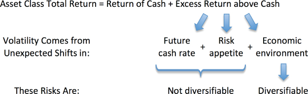
Figure 3.3 Asset Class Volatility Framework
Risky asset class returns are a function of the return of cash plus the excess return above cash. The return of cash is fairly stable through time. Excess returns are highly volatile. The volatility can be explained by three core fundamental drivers. Unanticipated movements in future cash rates is a risk that cannot be diversified away because it simultaneously impacts all asset class returns in a similar direction. Likewise, shifts in the general market appetite to take risk cannot be neutralized since they concurrently impact all asset classes in the same manner. Fortunately these undiversifiable risks do not negatively impact returns frequently and are short-lived (as will be fully explained in later chapters). You, as an investor, are compensated for taking this risk over the long run.
Conversely, an unexpected shift in the economic environment is a risk that is diversifiable. In fact, unexpected shifts in the economic environment represents the biggest hazard to investors of asset classes. Unlike the other two risks, which don't negatively impact returns too often and don't persist for long, this source of volatility can be diversified with a good balance of asset classes. This is only because different asset classes react differently to various economic climates. Moreover, you are not compensated for taking this risk. This makes it foolhardy to not try to properly neutralize this risk in constructing your asset allocation.
Your excess return will then depend on how the future rate of cash changes versus expectations, how general risk appetites shift, and how economic conditions actually transpire relative to what was originally expected. The goal of efficient portfolio construction is to capture the excess returns above cash offered by the first two parts and diversify away the risk of shifts in the economic environment. The whole objective of this book is to teach you how to diversify away the latter.
Note that I have isolated each of these three risks to help better explain them. In reality, several may hit at once. Risk appetite may decline at the same time as the economy weakens (which is typical). Thus, all asset classes take a hit from declining risk appetite, but stocks get a double whammy for falling growth while Treasuries receive a positive push from the same economic climate. These influences net out to result in positives and negatives for each asset class. The severity of each outcome also provides various degrees of influence by factor. If the economy materially weakens but risk appetite only falls a little, then the resulting asset class return would be determined by the more impactful factor.
Summary
Since we have determined that two of the three key sources of risk are not diversifiable, we will focus on the one that is diversifiable. Another way to think about asset allocation, and really the bottom line of this core chapter, is to appreciate the fact that each asset class is merely a package of different economic structural biases. Each asset class is impacted differently by unexpected shifts in growth and inflation. Some asset classes are positively influenced by rising growth, while others do better when growth underperforms expectations. There are asset classes that are biased to do well during rising inflationary environments and others that favor falling inflation. By isolating each asset class into the key factors that drive its returns (and therefore are the main cause of volatility) you will be analyzing portfolio construction from the appropriate perspective, which will lead to building a truly balanced portfolio. Figure 3.4 provides a visual of how each asset class is prepackaged with a bias toward these two key factors.
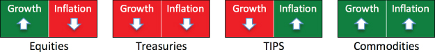
Figure 3.4 Economic Bias of Each Major Asset Class
Each asset class has some long-term expected return above cash and expected risk (or volatility around that long-term expected excess return). Both the long-term excess return and the volatility around that mean are somewhat reliable over time. It is the timing and direction of the variability that is highly uncertain (largely because of changes in the economic environment) and it is that uncertainty that you should try to neutralize. The key is to appreciate the underlying fundamental drivers of each investment's pricing and how it is linked directly to changes in the economic environment. These are reliable linkages because they are fundamental to the understanding of how investments work. For instance, equities are biased to outperform when growth is rising and when inflation is falling, as illustrated in Figure 3.4. Each asset class can be encapsulated using a similar analysis of its core fundamental economic bias.
With this core appreciation, the next step will be to dive into the details of how to view various asset classes through a balanced portfolio lens. It is important to see each asset class as having predisposed biases to unexpected shifts in economic conditions. The next five chapters will use this lens to explain why major asset classes have these inherent biases and why such a cause-effect relationship can be reliable. Chapter 4 starts with stocks (or equities) since that is the most common asset class in portfolios. Treasuries, TIPS, and commodities will follow in Chapters 5 through 7, respectively. Chapter 8 will use the same perspective to look at additional asset classes that you may want to consider for your balanced portfolio.
In each of these five chapters I begin by describing the conventional perspective of each asset class. This is the way most people think about and use this asset class. The focus of each chapter, however, is on assessing each asset class through the balanced portfolio perspective. With this new lens, you will see asset classes in a different light and more fully appreciate the benefits of each within the context of a well-balanced portfolio. How each asset class fits within the bigger picture rather than the attractiveness of each on its own should be the focus.