
Chapter 4
Viewing Stocks through a Balanced Portfolio Lens
An investment in a stock represents an equity ownership in a public company. This is why stocks are also referred to as equities. If you buy Google stock, for example, you instantly become a part owner of Google. As an owner of the company, you benefit from the company's profits, which are largely reflected in the price of the stock. The current price of the company's stock reflects future expectations of the company's fortunes. When profits surprise to the upside, the stock price rises, and vice versa. Google is one company. The broad stock market consists of a basket of publicly traded companies like Google.
Most investors already understand what a stock is and what makes up the stock market. However, as you will read in this chapter, the traditional perspective of how to think about stocks within a portfolio contains many oversights.
Introduction
When people ask how the market did today they are undoubtedly referring to the stock market, even though there are many markets to consider. The vast majority of headlines, analysis, and conversations are about how the stock market is faring. Bond, commodities, and real estate markets are just a few of many other major markets that do not seem to receive the same attention as stocks. For some reason our nation is gripped by the stock market (more so when it is going up than when it is not doing well, of course).
Consequently, equities are a staple in nearly every long-term portfolio. Those that are well balanced, as well as the imbalanced variety, are certain to contain some allocation of public companies. Thus, equities do not require a compelling argument for their inclusion in portfolios (unlike several of the other asset classes that will be covered later). Rather, the discussion needs to focus on why a heavy allocation to equities, as is commonplace in conventional portfolios, leads to portfolio imbalance.
The flaw centers on the way investors generally view stocks. Using a conventional lens, the high expected excess returns of stocks relative to other public markets attracts a high allocation in portfolios. Who wouldn't want more of the best performing asset (when viewed from this perspective)? There are several problems with this approach. First, stocks can underperform for uncomfortably long stretches of time. Moreover, the assumption that stocks offer higher returns is misleading when factoring in returns per unit of risk. Finally, a major drawback of an overweight to equities is the resulting portfolio's overdependence on the consistent returns of equities to produce successful results. All of these oversights will be fully explored in this chapter.
Ultimately, by discarding the conventional lens and analyzing equities using a balanced portfolio perspective, the appropriate role of equities will become more clear and the flaws in conventional logic far more apparent. Thus, the key emphasis in this chapter, and in the entire book, is to introduce a more thoughtful perspective that will help make it easier to build a balanced portfolio.
The Conventional View: Why Investors Own a Lot of Stocks
I begin with the perspective used by most. Investors are attracted to stocks largely because they offer one of the highest long-term average returns of the major publicly traded asset classes. Of the assets I discuss in this book, equities have achieved the highest average excess return above cash since 1927 (see Table 4.1).
Table 4.1 Annualized Asset Class Excess Returns (1927–2013)
| Asset Class | Average Excess Return | Average Volatility | Return-to-Risk Ratio |
| Equities | 5.6% | 19.2% | 0.29 |
| Intermediate-Term Bonds (Used in Conventional Portfolio) | 1.4% | 4.8% | 0.29 |
| Long-Term Treasuries | 1.4% | 10.0% | 0.14 |
| Long-Term TIPS | 4.6% | 10.6% | 0.43 |
| Commodities | 2.0% | 17.1% | 0.12 |
Cash returns from 1927 to 2013 averaged 3.8 percent per year. Thus, total returns can be approximated by adding 3.8 percent to the average excess returns provided above.
Equity returns stand out on this list when looking at historical returns. Most of the other popular options have produced much lower returns over time. Long-term TIPS, which come in second, have only been around since 1997. Thus, they don't have stocks' historical record and don't garner as much attention.
Conventional wisdom also recognizes that along with higher returns, stocks come with greater risk. This means that their returns fluctuate over time more than other assets. However, the assumption is that if you are willing to take the risk and have a long enough time horizon, then you should own a high allocation to stocks. This is how you achieve higher returns over time. Based on conventional logic, it is generally the time horizon and your risk tolerance that dictate the proportion equities represent in your portfolio. The conventional view holds that if you are younger, you should own more stocks; if you are retired, a smaller allocation to equities is appropriate. Many professionals simplify the math by arguing that you can take 100 and subtract your age as a general guideline to determine the equity allocation. If you are 30 years old, then 70 percent stocks (100 minus 30) is about right. If you are 70, then a 30 percent allocation is probably appropriate.
Another key factor that is traditionally used is your emotional risk tolerance. How much volatility can you handle? If your portfolio lost 20 percent in a year, would you feel compelled to sell at the low or would you be able to hold on and wait for the cycle to reverse? Can you stomach the roller coaster ride or are you more of a merry-go-round type? The rule of thumb holds that the more risk averse you feel, the fewer equities you should own.
One final traditional approach to the equity allocation decision is based on liquidity: If you might need to liquidate your equities over a shorter time frame (typically defined as five years or shorter), then a lower allocation to stocks is prudent. Again, the main logic is based on the amount of time that you are able to hold on to your stocks. The longer you can avoid selling, the more stocks you should own because stocks outperform over the long run.
The conventional asset allocator uses the previously described rationale to identify the right allocation to stocks in a portfolio. The net result of this common mindset and approach is a portfolio that generally contains a high allocation to equities. This bias is so prevalent that a 60/40 portfolio is widely considered to be balanced, even though it maintains a 60 percent allocation in one asset. Three major oversights in this thinking should be considered.
Oversight #1: The Risk of Long-Term Underperformance in Stocks
Stocks are viewed as the ultimate long-term asset. Conventional wisdom holds that the longer your time horizon, the more equities you should own. The major flaw in this logic is that stocks can perform extremely poorly for a very long period of time. In essence, the long run may be too long for you to wait.
Stocks only offer higher average returns over the long run. Averages can be very misleading. Imagine an asset class that averages 10 percent per year, but only delivers positive returns once every 100 years. It earns 0 percent every year with the exception of once a century, when it produces a positive 1,000 percent return. An attractive average return is not terribly useful in this extreme example. By investing in this asset class you will most likely earn 0 percent regardless of the average. Obviously stocks generate more reliable and consistent returns than indicated in this example, but the difference is probably less stark than you realize.
The reality is that the stock market is highly cyclical. It enjoys great runs followed by long episodes of severe underperformance. These prolonged periods are not just the three- to seven-year period that is commonly referred to as the full market cycle. They can last 15 to 20 years or longer, which by anyone's definition is a very long time. Regardless of your level of conviction about investing for the long run, a couple of decades of underperformance can truly test your patience. In reality, five years is a long time for most people and it seems as if the time horizon has been shrinking, not increasing, over the years. Indeed, it appears that we live in a world that demands immediate gratification. The trend certainly does not support greater patience over time. Every major market move is highlighted and exploited by the growing number of media outlets, which has made it quite challenging to try to maintain a long-term focus.
Table 4.2 provides a summary of the major long-term equity market cycles since 1927. This table breaks down the excess returns of equities into long-term periods from peak to trough and then back to the next peak. The main message is there exist lengthy periods of great results and drawn-out periods of near zero excess returns.
Table 4.2 Long-Term Equity Cycles (1927–2013)
| Period | Annualized Equity Excess Returns | % of Total Time |
| 1927–1929 | 41.9% | 2% |
| 1929–1948 | 0.4% | 22% |
| 1948–1966 | 13.5% | 21% |
| 1966–1982 | –3.0% | 19% |
| 1982–2000 | 12.7% | 21% |
| 2000–2013 | 1.2% | 16% |
| Entire Period | 5.6% | 43% above average |
| 57% below average |
Notice the time periods presented in the table. These are typically 15 to 20 year cycles. The up periods (1927–1929, 1948–1966, and 1982–2000) offer significant gains. However, the down cycles leave much to be desired. In most cases, the down legs have provided negative excess returns above cash, meaning that cash beat stocks for a long period of time lasting a decade or more. These bear markets account for 57 percent of the measurement period since 1927. In other words, we have lived through a secular bear market in stocks for more than half of history. Most people miss these obvious cycles simply because they are viewing the market too closely by focusing on 3- to 5-year cycles (which may feel like a long time to them).
The other important point to draw from Table 4.2 is the randomness of the cycles. It may appear that every 15 to 20 years the cycle turns, so you just need to wait another several years and then you can load up on equities. The randomness lies in the timing of the inflection points in the cycles. The table makes it look like the transitions occur regularly and smoothly. In reality, each of these bull and bear markets contains mini market cycles within them. Thus, you really don't know if the cycle has turned until a far later point in time.
The key lesson is that the stock market goes through very long periods during which it underperforms expectations and its average long-term returns. By concluding that you can afford to take risk and then overweighting equities, you are taking a huge risk in the timing of your decision. If you happen to pick the wrong half of time, then you will likely be quite disappointed with your asset allocation decision. Would you really be willing to flip a coin to determine the outcome of your portfolio? Heads you win and tails you lose. This is not the most prudent and rational approach, particularly since having a balanced portfolio (as will be shown later) would largely alleviate these risks.
Another way to analyze the long-term trends of the stock market through history is to observe rolling 10-year returns since 1927. If we assume that 10 years is a long time, then it would be informative to see the historical range of 10-year returns based on all the possible starting points since 1927. The percentage of time that the rolling 10-year returns were above and below average is also instructive. The results are presented both in chart (Figure 4.1) and table (Table 4.3) formats. Figure 4.1 illustrates that stocks have spent long stretches above and below their mean excess return of 5.6 percent. The chart uses 10-year rolling periods.

Figure 4.1 10-Year Rolling Equity Excess Returns
Table 4.3 segregates the results by the percentage of time spent above and below the average excess returns.
Table 4.3 10-Year Rolling Equity Excess Returns (1927–2013)
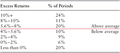
Based on this data, if you randomly picked a 10-year period that occurred sometime between 1927 and today, the odds that the returns you would earn from equities would fall below cash is about 20 percent. This means that the stock market underperformed cash for 10 years! From a probability perspective, this implies that you have a one in five chance of picking a very bad 10-year period in which to invest in equities. Nearly half of the rolling 10-year periods produced below average returns, meaning that you would have been disappointed with the results. Since 10 years is a relatively long time for most people, this is a fact that should not be quickly dismissed. Ten years of underperformance is typically enough to cause significant financial pain. It is also sufficiently prolonged as to reasonably produce shifts in investor behavior. A bad year or two may be easily forgotten, but 10 years of dreadful results can leave a lasting impression and cause second thoughts about original assumptions.
It is also unrealistic for you to assume that you possess the prescience to avoid the bad times. You might think that you will certainly identify red flags before the fact and successfully sidestep bear markets. Your actual experience, you might argue, will likely be different from that listed in Table 4.3. The problem with this perspective is that the reality suggests exactly the opposite conclusion. That is, most investors are actually predisposed to jump in, not sell, before major bear markets. In fact, the odds of investors overweighting stocks during the next 10-year bear market is probably greater than the straight 20 percent odds would imply. This is because investors are saddled with the disadvantage of emotion. Even the most collected, rational investors are hardwired emotionally to want to do the wrong thing at the wrong time. Why does this continue to happen? The answer, in short, can be largely explained by the human motivations of fear and greed. Greed causes investors to chase returns after an upturn, while fear forces them to sell underperforming investments for worry that the poor results will continue.
The normal cycle typically repeats as follows: The stock market begins to string together impressive returns, optimism builds, and strong animal spirits develop. Strong returns attract capital, which pushes prices even higher. Momentum ensues and eventually causes long-time bears to succumb to the pressure of sitting on the sidelines and watching friends achieve great investment success with little effort. During the late stages of these long-term bull markets, manias form and fundamentals are largely ignored while talk of “this time is different” dominates. Widespread overconfidence, significant risk taking, excess leverage, or all three often signal that the end is near.
Fear begins when markets turn for the worse, often without sufficient warning. Just as was the case on the upside, recent returns are extrapolated into the future as hope of a market rebound fades. Fundamentals once again become important and risk tolerance reverts to the opposite extreme. Risk takers and highly leveraged investors are punished as too many rush for too few exits. Prices suffer and a long-term bear market has begun. The excesses are slowly worked off until the market becomes attractive once again, just before the inception of the next bull market (which has tended to coincide with widespread pessimism about future prospects).
This may sound like an oversimplification. However, since these long-term periods tend to last as long as 15 to 20 years, there is enough time between bull and bear markets for investors to forget their mistakes and fall into the same traps over and over again. In reality, these long-term periods include various shorter-term bull and bear markets within them, which makes them even more difficult to distinguish.
A recent example of these cycles will perhaps resonate with you. The last set of 10-year rolling periods during which equities earned a negative excess return occurred in the 1998 to 2000 start period (therefore ending from 2008 to 2010). You may recall the level of general optimism during the dot-com Internet boom. In fact, it was a time marked by substantial exuberance over the forward-looking prospects of the economy and the stock market. Many investors loaded up on stocks that promised to grow to the sky. That period may have marked one of the peaks in U.S. infatuation with the stock market.
Oversight #2: Equities Are Just Prepackaged to Offer Higher Returns
The conventional view's core argument is that stocks offer higher expected returns over the long run. A major flaw with this assumption is that this is only true because stocks are prepackaged to offer attractive returns. When I say prepackaged, I mean to describe the structure in which this asset class is normally available to investors. If you bought a broad U.S. stock market index fund (such as the S&P 500 Index) in 1927 and held on until today, you would have earned attractive average excess returns. Notice, however, that other asset classes have achieved a similar long-term return-to-risk ratio as equities.
For instance, the other component of the traditional 60/40 mix—intermediate-term bonds (also known as core bonds)—has achieved a lower excess return than stocks (1.4 versus 5.9 percent), but they have also experienced lower volatility (4.8 versus 19.2 percent). The key is that the ratio of return to risk was about the same as that of the stock market (approximately 0.3 each). This means that you could have levered core bonds since 1927 to earn the same return with the same risk as stocks. The leverage could be achieved by investing in futures of the core bond index, the Barclays Aggregate, to package the asset differently. The asset is prepackaged to provide lower returns with lower risk, but you can easily change that. You don't have to take this asset class off the shelf since you have the ability to customize it to better fit your needs. Most investors neither know they can do this nor would take advantage of it because it sounds risky and unconventional. With recent advancements and growth of investment products, there are prepackaged exchange traded funds or mutual funds that you can purchase just like a stock or bond fund that provide such characteristics. Thus, it is easier than ever to take advantage of this inefficiency.
Regardless of your aversion to lever other asset classes, the bottom line is that higher returns should not be the main reason you buy equities. You can get the same return from bonds or other asset classes by restructuring them. Likewise if you are looking for lower risk and return than that offered by equities, you can simply add cash to the portfolio to bring down the volatility and returns. This is another way of customizing the asset class. Again, I am not espousing such a strategy, but it is an option you should be aware of.
Oversight #3: The Conventional Approach Results in Imbalanced Portfolios
The third major reason to conclude that the conventional perspective of equities is highly flawed is because a simple, high-level review of the portfolios that result from such an approach tells us they are grossly imbalanced. An important question to ask is how do portfolios that own a high allocation to stocks generally behave? In other words, if you followed the conventional mind-set of adding stocks to a portfolio merely because of their high expected returns, then what might your portfolio end up looking like?
One simple way to observe the resulting portfolio characteristics is by comparing the correlation of the portfolio to the stock market. Correlation is just a statistical method of measuring how two streams of returns are co-related. Correlation data can be used to compare the dependence of traditional portfolios to the success of equities. A high correlation means that the two generally move in sync. A negative correlation signals that the two perform the opposite of one another. They don't have to go up and down to the same degree so long as they move in the same direction. Thus, the correlation can be as high as +100 percent (or 1.0) or as low as −100 percent (or −1.0). A correlation of 0 indicates no correlation. Any number higher than 80 percent suggests a very high correlation between the two return streams you are comparing.
The thinking is that if the total portfolio is highly correlated to the stock market, then it can't be considered well balanced because we already know that the stock market can easily experience prolonged periods of underperformance. Table 4.4 lists the correlation of various conventional portfolio mixes to the stock market. These portfolio allocations represent typical outputs using conventional inputs. My objective is for you to appreciate the extraordinarily high correlation that all of the conventional portfolios have to equities. Note that the data used goes back to 1927, so this is not an aberration.
Table 4.4 Conventional Portfolio Correlations to Equities (1927–2013)
| Asset Allocation | |||
| Portfolio | Equities | Fixed Income | Correlation with Equities |
| Aggressive | 90% | 10% | 100% |
| Moderately Aggressive | 75% | 25% | 100% |
| Moderate | 60% | 40% | 99% |
| Moderately Conservative | 45% | 55% | 96% |
| Conservative | 30% | 70% | 88% |
What the data shows is that even a portfolio commonly viewed as conservative using conventional methods is highly correlated to the stock market. In other words, you may think that your portfolio is conservative but its results are almost entirely conditioned on how well the stock market performs. The more aggressive mixes are even worse. Consider that a so-called moderate allocation of 60/40, which is widely considered to be a traditional portfolio allocation, is 99 percent correlated to the stock market. Clearly, this is not well balanced! Believe it or not, most investment professionals are completely unaware of these simple-to-calculate statistics. Indeed, most would be absolutely shocked at these figures and would probably not believe them to be true (you can check for yourself using a simple formula in Excel).
If you were to ask a business school professor what he thought the correlation would be between a 60/40 equity/fixed income portfolio and a 100 percent equity portfolio he may apply the following logic (which he probably learned in business school and likely teaches his students now). When you take two asset classes that have a low correlation to one another—such as stocks and bonds—the correlation of the combined portfolio should be reduced due to the benefits of diversification. Thus, if you own 60 percent stocks and 40 percent bonds, then the correlation between that mix and one with all stocks should be less than 60 percent. The logic suggests that this must be true because you only own 60 percent of the asset class that you are comparing to a portfolio that consists of 100 percent of the same asset. Because the other 40 percent is invested in something you know has low correlation to the 60 percent holding, then the combined portfolio should benefit from this diversification to result in a mix that has a correlation less than 60 percent. This thought sequence may sound intuitive, but it is completely erroneous.
How can this be? In order to see how obvious this result is you must ensure that you are looking through the correct lens. The traditional approach would leave you confused, as it does most investors. If instead you observe these portfolios from a balanced portfolio standpoint, the results will become evident.
The Balanced Portfolio View: How to Think About Equities
Equities are very volatile and can go through decades of underperformance, as you just read. Therefore, it makes much less sense to focus on the returns than it does to try to understand what drives the returns. If you emphasize the high expected returns and build a portfolio with the expectation that you will earn those returns, then you will be putting yourself in the unenviable position of having too high a probability of underachieving your expectations. Moreover, if the success of your portfolio requires equities to perform well, then you are effectively putting all of your eggs in the equity basket. Recall that most portfolio combinations using the conventional perspective lead to portfolios that have a high correlation to equities, which signifies an overreliance on this asset class. There has to be a better approach.
Fortunately, there is. In order to see asset classes through the lens of a balanced portfolio, you need to consider each asset class in two ways. First (as explained in the last chapter) the key driver of asset class returns, including equities, is unexpected shifts in the economic climate. The economic drivers to emphasize include unexpected changes in growth and inflation. Second, the volatility of each asset class matters. This is because the more volatile the asset the greater the impact to the total portfolio.
In this chapter, equities will be examined through the lens that looks at them in terms of their economic bias and volatility. By understanding what influences the returns of equities within this context, you will establish a solid foundation on which to make a well-informed asset allocation decision. You will then be armed with the insight needed to build a well-balanced mix of asset classes and to better understand the role of equities within the total portfolio.
Economic Bias: Rising Growth Bias of Stocks
Positive growth is a huge plus for equities because it directly impacts the top-line revenues of most companies. This is due to the stronger economic activity that has led to increased spending. More spending results in higher company revenues since someone's spending is someone else's income and that process generally runs through companies. Higher revenues, all else being equal, produce greater profits for corporations. Better than expected profits generate upward pressure on stock prices since ultimately it is company's profits that make a company worth something. When the economy grows faster than discounted, this logical sequence typically leads to higher equity prices because the old price had not reflected the improved conditions.
As a result, equity prices are impacted by unexpected shifts in economic growth. When growth comes in better than conditions that had already been discounted in the stock price, then a positive influence results. The opposite is also true: Negative surprises generally lead to price declines.
Economic Bias: Falling Inflation Benefit to Equities
There are two parts of the profit equation: revenues and profit margins. Rising growth positively influences revenues, while falling inflation can improve profit margins. Inflation is a measure of the increase in the cost of goods and services. These same items are inputs into the cost of doing business for corporations. Moreover, falling inflation exerts downward pressure on interest rates, which also benefits companies as the cost of borrowing money declines. As company costs decline (both from lower borrowing and input costs), profit margins increase, all else being equal. Thus, if growth transpires as expected and inflation falls more than expected, then revenues may come in as priced but the margins may improve. The net result is positive because profits have increased more than discounted. Note that if growth is rising and inflation is falling simultaneously, then such an economic outcome marks a double positive for stocks and generally results in the best overall environment for this asset class. Such an economic outcome largely explained the unprecedented equity returns during the 1980s and 1990s bull market. Consequently, unexpected decreases in inflation positively impact stock prices and vice versa.
Combining the Two Economic Biases of Equities
Together, the rational cause-effect relationship between unexpected shifts in growth and inflation reliably impacts stock prices and results in price fluctuations over time. Moreover, so-called good environments characterized by rising growth or falling inflation relative to expectations generally exhibit stronger equity returns than so-called bad periods during which the opposite sets of conditions exist. Not only do the conceptual linkages make sense, long-term historical data also supports this cause-effect relationship. The historical data backing this outcome are summarized in Table 4.5.
Table 4.5 Annualized Equity Excess Returns by Economic Environment (1927–2013)
| Annualized Excess Return for All Periods (Good and Bad) | Good Environment (Avg. Excess Return) | Bad Environment (Avg. Excess Return) |
| 5.6% | Rising growth (10.7%) | Rising inflation (1.9%) |
| Falling inflation (9.5%) | Falling growth (1.3%) |
Source: Bloomberg and Bridgewater. Methodology used to determine whether growth and inflation are rising or falling: current growth or inflation rate compared to average of the trailing 12-month period. If the current rate (of growth/inflation) is higher, then that is considered a rising growth/inflation period and vice versa. The logic is based on the observation that most people expect the future to closely resemble the recent trend line.
Notice how much better equities have historically performed during good economic climates versus bad times. You may also recognize that the average excess return since 1927 of 5.6 percent is just about midway between the positive growth environment returns (10.7 percent) and the negative growth climate returns (1.3 percent). The same observation holds for falling inflation periods (9.5 percent) and rising inflationary environments (1.9 percent). The reason the average is almost exactly in the middle of the two ends of the spectrum is because of the frequency of each economic environment. As I've mentioned before, each economic climate occurs roughly half the time because what really matters is how the future transpires relative to what had been expected to occur. In fact, about half of the months since 1927 can be characterized as rising growth and about half as falling growth. Rising inflation and falling inflation each also cover about half of the measured environments.
Figure 4.2 provides the historical rolling 10-year excess returns of equities to help you observe the results over long time horizons. Periods of outperformance understandably occur during environments characterized by either rising growth or falling inflation (or both). Likewise, long-term underperforming years occurred during falling growth or rising inflationary economic climates.

Figure 4.2 10-Year Rolling Equity Excess Returns versus Growth and Inflation
The Importance of Volatility
The economic bias of equities is a critical input into assessing how equities fit within a truly balanced portfolio. The second important input into the asset allocation decision-making process is to factor in the volatility of equities. Why does the volatility of an asset class make a difference in how it fits within the balanced portfolio framework?
Remember that the objective is to build a portfolio using various asset classes to capture the excess returns offered by them with as little variability around that mean as possible. Therefore, in order to determine the allocation of each to own you need to think about how much each asset class is likely to move around its mean. Those asset classes that are highly volatile will fluctuate around their average more than those that are less volatile. The reason that assessing volatility is a key step in the process is because it is this measure that identifies the magnitude of the fluctuations around the average excess return. The more an asset class moves around its mean, the greater the impact to the total portfolio. Economic bias tells us when the asset class is biased to outperform or underperform its average return. Volatility tells us how much it is predisposed to fluctuate around its mean. Both characteristics are important inputs into the balanced portfolio decision-making process, since both have a direct impact on the return pattern of the total portfolio.
Consider an extreme example to help understand the significance of volatility in the balanced portfolio framework. Imagine two asset classes: One is super volatile and the other has very low price volatility. Further, assume that the economic bias of both is identical. Consider the difference in impact to your total portfolio if you included one asset class versus the other. With the super volatile asset class your total portfolio would perform very well during economic environments during which the asset class is biased to do well and exceptionally poorly during the opposite climates. On the other hand, the low-volatility asset class has much less impact on the total portfolio even though it shares the exact same economic bias as the first asset class. Why is this? Since low volatility means that the returns do not fluctuate materially from year to year, then a return during a good year will not be much better than a return in a bad year. Conversely, a highly volatile asset will experience huge swings in its returns. Years characterized by positive economic environments will produce great returns, and negative environments will result in very poor returns. Putting numbers to it, the high-volatility asset may return +30 percent or –30 percent while the low-volatility version may return +3 percent or –3 percent. Obviously the wider swings in returns will cause greater fluctuations in the returns of the total portfolio (assuming the same allocation to each).
Of course, volatility will change over time. There are periods during which equities will experience greater volatility and other times when the volatility will be lower. The goal here is not to predict the exact volatility over your investment period. Rather, try to view volatility at a broad level. Perhaps you can characterize equities as containing high volatility relative to other asset classes such as bonds, which may have low or medium volatility (longer-maturity bonds have more volatility than shorter-maturity bonds). Do not attempt precision. It is nearly impossible to predict the exact volatility of the future based on the past. However, a range of volatility expectations or a broad categorization of future volatility is likely to yield a more successful approach.
At this point, the key insight you should appreciate as we go through each asset class is that the volatility of each is an important factor when considering how it fits within the balanced portfolio. Along with the economic bias of the asset class, these two inputs are the key criteria that will be used to construct a truly balanced asset allocation.
In terms of equities, you know that stocks are likely to outperform their average excess return when growth is rising, when inflation is falling, or when both conditions are present. You can also determine with some reliability roughly how much above or below the mean stocks are probably going to oscillate on average. This is clearly not an exact science, but you can reasonably anticipate that stocks will experience greater volatility than bonds, as an example, both because of actual experience and because conceptually it makes sense for this to be the case. Furthermore, common sense and history suggest that the bigger the shock from shifts in the economic climate, the bigger the moves around the average. For instance, if growth significantly outperforms expectations, then the upside for a pro-growth asset class will likely be material (just as the downside would be drastic for a falling growth biased asset class). You saw this in 2009 as expectations for growth were very weak following the financial crisis. Equities delivered very strong returns as economic growth, while not strong, far exceeded overly pessimistic expectations. Conversely, if growth comes in just slightly stronger than discounted, then the upswing above the average may be more muted.
Recall that one of the major flaws in the conventional approach to asset allocation is the noticeable imbalance in the resulting portfolios from such a process. With this understanding of the importance of volatility, you are now better positioned to appreciate why the conventional mind-set has led to such poorly balanced portfolios. We have already discussed the oversight in conventional thinking of not considering the economic bias of each asset class. The second missing element in the conventional analysis is the volatility of the asset classes in terms of how that factor influences the total portfolio.
With this new lens you can see why 60/40 is so weakly balanced. If you take two assets and one has high volatility and the other has low risk, then the more volatile of the two will obviously impact the total results more. Think of the 60/40 portfolio within this context. The 60 is four times as volatile as the 40 and will therefore drive the total portfolio returns. When stocks perform well, the 60/40 mix does well and vice versa. The returns of the low-volatility bonds effectively don't make much of a difference to the portfolio's overall results because they don't move around enough. By overallocating to the more volatile asset class, you actually hurt the balance in the portfolio even more. As I will describe further in the chapters about Treasuries and TIPS, this is one reason owning longer-duration, more volatile bonds actually improves the balance in the portfolio (even though individually they are considered more risky by conventional measures).
In a nutshell, the simplest way to view the equity asset class within the newly introduced balanced portfolio framework is as depicted in Figure 4.3.

Figure 4.3 The Economic Bias of Equities
When I look at an equity asset class, I visualize these two boxes. In fact, the boxes are more important than the equity label, since the boxes represent the biases of the asset class. A different asset class with the same biases should be viewed the same as equities, since the key drivers of returns are the crucial input into building a balanced portfolio (as will be shown later).
Equities are predisposed, for perfectly rational reasons, to perform better than average when growth is rising and when inflation is falling. When both occur, that is the best environment for stocks. When the opposite climate dominates, that predictably results in the worst outcomes. There are other variations too. Sometimes growth, inflation, or both can come in as expected and therefore not materially influence the results. Other times, these factors may shift meaningfully from trend and significantly influence returns. In these cases, the factor that dominates more from expectations will generally have the greater influence on the price. For example, if growth is in line and inflation falls, then the inflation factor will dominate for that period. In the case of equities, since it is a falling inflation asset, such an economic outcome would be favorable. The data supports this outcome, but, more importantly, because of the logic described above, this cause-effect relationship simply makes sense.
Ultimately, you don't need to guess the economic outcomes. You merely need to have confidence in the cause-effect relationships between whatever the economic result and the general impact to equities. If growth unexpectedly accelerates, then equities are biased to outperform their average returns. If inflation falls, then equities are biased to outperform. It is the relationship that should be the focus rather than the outcome. Adding to this, the volatility of equities tells us roughly how much the price can generally be expected to fluctuate around its average long-term returns.
Thus, together, we have two reliable factors that do not change much over time. We know when equities tend to perform well and we know how much better than average they are predisposed to perform during these environments. These two key insights are far more reliable characteristics of equities than their absolute returns during any forward-looking period. If the foundations on which you are basing the all-important asset allocation decision are unstable, then the resulting portfolio is likely to also be unstable. If the key input in the process is a high expected return of equities, then the core input is far more likely to disappoint than if the main reason for using equities in a portfolio is because of its more reliable cause-effect relationship to various economic outcomes and its general volatility over time.
When you view equities using this perspective, the portfolio construction process naturally leads you down a very different path. However, if you view equities using conventional logic, then the focus will be on returns. Since equity returns are inherently unreliable because they can produce unacceptably low returns for decades at a time, why would you base the critical asset allocation decision on this factor? Rather, it seems more prudent to depend on the cause-effect relationship between growth and inflation conditions and equity returns since that connection is logical and far more reliable over time. Following this methodology, how then should equities be considered within a total portfolio? What is the role of equities within a total portfolio context using the balanced portfolio framework? To these vital questions I now turn.
The Role of Equities in a Truly Balanced Portfolio
Based on its bias to rising growth and falling inflation, equities fulfill an important part of a well-balanced portfolio. Since growth and inflation are the primary drivers of asset class returns, a portfolio of asset classes should allocate among asset classes in a way that tries to neutralize these primary drivers. After covering the major asset classes in the next several chapters, I will explain in detail how to accomplish this ultimate objective. For now, I will focus on how you should think about equities and how this particular asset class fits within the bigger picture.
Since you know that unexpected shifts in growth and inflation are largely responsible for changes in individual asset class pricing, a required characteristic of a truly balanced portfolio is that it does not share this attribute. That is, the underlying asset classes may be impacted by economic shifts, but a cleverly constructed mix of them should result in much greater stability at the total portfolio level. The stability comes from a total portfolio that has no inherent bias to growth and inflation. If the portfolio is not predisposed to perform better or worse during rising growth or falling growth, or rising inflation or falling inflation, then that represents true balance.
Equities play a role in reaching that ultimate objective. Since equities do well during periods of rising growth and falling inflation, then it naturally follows that this asset class checks off those boxes. Thus, by including equities in a portfolio, if the economy is surprisingly strong or if inflation unexpectedly drops, then the portfolio will have a component (equities) that will be biased to deliver strong results. This outperformance will likely offset underperformance in other parts of the portfolio, which are biased to do well during opposite economic environments.
Conventional portfolios clearly own too high a proportion of equities. However, my goal is not to talk you out of owning any equities. The argument should not be taken too far. The objective is to keep good balance and that requires a deep understanding of the key drivers of asset class returns. Even if you are a very conservative investor and feel that the volatility of the stock market is too much to bear, you should probably still own some equities. If you take it to the other extreme and avoid the entire asset class, then you would be leaving your portfolio exposed to the environments in which equities outperform. The logic works both ways. This may sound a little counterintuitive since stocks are far riskier than bonds. The problem is that bonds, like stocks, can go through long bear markets as well. Bonds have their own economic bias and if the environment plays out in an adverse direction, then bonds can perform quite poorly for a prolonged interval. This is what happened during the 1970s and early 1980s as interest rates surged from 5 percent to 15 percent when inflation far exceeded expectations. In that scenario stocks would not have helped as they too underperformed, but the inflation hedges would have added significant value. If interest rates rise again in the future, it may be because economic growth outperformed discounted levels. In that case, equities may actually fare well and provide some offset to bond market weakness. We saw this dynamic play out in 2013 as equities performed strongly while bonds lost money.
Summary
Most investors start with the assumption that they should own as high a proportion of equities as they can handle because stocks offer the highest expected return of the major asset classes. Then bonds are added to fill the remainder and lower the overall volatility of the portfolio. My main aim in this chapter was to emphasize evaluating the equity allocation decision from a different perspective. You should think about it in balanced terms. Treat the equity decision the same as you would the other asset classes. Ask in what economic environments is it biased to outperform and how does it fit within a balanced portfolio framework.
Using the conventional lens to view equities, you would conclude that a high allocation to this asset is warranted. Equities have historically produced high expected returns relative to most other liquid asset classes. Conventional wisdom holds that if the objective is to achieve strong returns, then you must own a lot of stocks. This argument sounds intuitive and logical, but only if viewed from a conventional perspective.
The reason you now know that the conventional view is flawed is because of major oversights in some of its core assumptions. Stocks can underperform for far longer than most investors' patience can bear. Additionally, the assumption that stocks offer higher returns can easily be debunked by adding leverage to other asset classes to match the expected return of stocks. Finally, you understand that a portfolio created using this approach results in significant imbalance: If the output of the process is poor, then there must be something wrong with the input. To fully appreciate the flaws with the input, you need to remove the conventional lens and view asset classes—equities in this case—through a different lens.
I refer to the lens that is being introduced in this book as the balanced portfolio lens because our objective is to build a balanced portfolio. You learned in previous chapters that unexpected shifts in economic conditions (growth and inflation) are largely responsible for variations in asset class returns. Most importantly, this is the factor that can cause the most harm but also the factor that is diversifiable. Thus, by looking at each asset class through a lens that involves an analysis of its economic bias, then we are better positioned to construct a well-balanced portfolio. Notice that expected returns are not part of the process. The goal is merely to identify the economic bias of each asset class and put them together so that the total portfolio is neutral to shifts in growth and inflation.
Within this context, equities are rising growth and falling inflation assets. For good reasons, these biases are reliable indicators that can be used to build a balanced portfolio. In the next four chapters, a similar analysis of Treasuries, TIPS, commodities, and several other asset classes will be developed.