
Chapter 9
How to Build a Balanced Portfolio
Conceptual Framework
This chapter is about how to achieve a balanced portfolio. For reasons I will explain here, the best portfolio is the most balanced portfolio. What I am going to show you was discovered by Ray Dalio and his team at Bridgewater.
It is easy to make money when economic growth is rising and the stock market is soaring. You really don't need to read a book to enjoy success during those environments. However, the key to successful long-term investing is whether you are able to survive economic troughs. How does your portfolio perform during the difficult times? How vulnerable is it to adverse economic climates, and are the potential dips in asset value so significant as to result in catastrophic losses? The framework behind construction of a balanced portfolio is to account for all contingencies so that you have a good chance of surviving the inevitable bad times and participating in strong economic environments.
More specifically, the idea behind a balanced portfolio is to achieve steady returns over the long run and to minimize the risk of major drawdowns and prolonged periods of underperformance. In order to achieve these objectives, you need to first identify where returns come from and why they are volatile. Earlier in the book I identified the key drivers of asset class returns. I established that returns fluctuate due to unexpected changes that inevitably occur in the following three areas:
- Economic environment (in terms of growth and inflation)
- General risk appetite
- Future cash rate
Further, I explained that unexpected shifts in the economic environment occur frequently and can last a very long time. These surprises are responsible for producing significant underperformance in asset class returns both as it relates to severity (peak to trough drawdowns) and longevity (the length of an extended period of poor returns). Recall that these two negative outcomes are the two major downside risks that we are trying to minimize in constructing a balanced portfolio. We want good returns, but want to avoid big losses and long-term underperformance. Since unexpected shifts in the economic environment are largely responsible for these two outcomes that we seek to avoid, it makes a lot of sense to think of building a portfolio from this perspective. Fortunately, and perhaps most importantly, the existence of unanticipated shifts in the economic climate is a risk that can be diversified with a proper asset allocation.
The other two risks negatively impact asset class returns infrequently and for short time frames. Since exposure to these risks is inherent in earning excess returns above cash, they are not something you can diversify away (without giving up the excess returns taking these risks provides). You have to live with the potential downside that may result from these forces when you invest your risk-free cash into risky asset classes in order to earn the excess returns—or risk premiums—they offer.
Based on these fundamental understandings, it is sensible that the portfolio construction process should be rooted in the philosophy of trying to neutralize the risk of unexpected shifts in the economic environment. This is the biggest risk to investors in asset classes and it can be diversified with a thoughtful asset allocation. The purpose of this chapter is to establish the conceptual framework for building a balanced asset allocation. The main objective is to efficiently capture the excess returns (or risk premiums) above cash offered by the various asset classes by appreciating the cause-effect linkages between changes in the environment and their returns.
Ray Dalio developed the understanding of asset class drivers and the portfolio structuring framework that I have been describing, in particular the idea of risk-adjusting assets and the identification of growth and inflation as the primary environmental drivers of asset class returns. He always believed that it is important to “know where neutral is,” by which he means to know what portfolio you would hold if you had no opinions about where the markets were going. Once you know where neutral is—that is, what a balanced portfolio is—you should tactically deviate from it only if you are smart enough to bet against other market participants with respect to the direction of the market. This neutral asset allocation mix is also called one's strategic asset allocation mix. It is based on the knowledge of how markets are likely to move in relation to each other. For example, if you don't know the direction of the markets, but you do know that when one market goes up another goes down, then you know something important about how to achieve a balanced portfolio.
These concepts form the basis of Bridgewater's All Weather approach to asset allocation, which Ray Dalio developed to be the permanent asset allocation mix for the inheritance money for his children and grandchildren, and that led Bridgewater to launch its All Weather strategy in 1996 and manage it for some of the largest institutional pools of capital in the world. It was other managers drawing from the All Weather principles in various ways that gave the rise to the recent risk parity movement. The framework for building a balanced portfolio I describe in this chapter draws from my understanding of All Weather, but is not meant to reflect exactly how Bridgewater actually manages its strategy.
Introduction: Two Simple Questions
There are essentially two key questions that you should ask yourself when deciding how to build a balanced portfolio:
- Which asset classes should I own?
- How much should I invest in each?
Putting together a portfolio is truly that simple. There is no need to overly complicate the process, as is far too common in the investment community. Anyone can do this well, but the thought process for each of these steps should be based on a solid logical foundation. Furthermore, you need to get both parts right. If you don't own the right asset classes, then you can't get balanced, because you are likely to do really well during the economic environments that you are heavily exposed to and poorly during other economic climates. If you don't weight the asset classes properly, then the positive returns of the winners may not be large enough to offset the negatives of the losers during certain economic periods.
Question One: Which Asset Classes?
Because we are trying to build a portfolio that in aggregate is not biased to outperform or underperform in any growth or inflation environment, the first step is to identify asset classes in terms of their individual economic sensitivities. When you look at asset classes, you need to consider them by their economic biases so that you have the right information to put together a portfolio of these assets that is neutral to the economic environment. Think of each asset class as being prepackaged to provide exposure to various economic climates. Try to see asset classes in this light.
Going back to the fundamental understanding of what drives asset class returns and the goal of neutralizing these factors, the strategy should be to identify asset classes that are biased to outperform during different economic environments. Some do well during rising growth periods and some do well during falling growth periods; some favor rising inflation and others falling inflation. Such an approach provides the opportunity for the portfolio to own something that is biased to perform well regardless of which economic climate dominates in the future. If the economy suddenly and unexpectedly weakens (as it is predisposed to do), then such an outcome would probably result in losses in pro-growth assets. However, by owning investments that have a falling growth bias and which outperform their average excess return in such an environment, then at least one segment of the portfolio would potentially offer a positive offset to the negative returns. The same logic holds for the other economic climates.
The crucial insight to appreciate is that the same environment that causes one asset class to underperform its mean simultaneously helps another outperform its average. Even though shifts in the environment may be difficult to anticipate, it is the understanding of what causes the excess return to fluctuate around its mean that is the instructive part of the analysis. You do not have to know when an asset class's excess return is going to perform well or poorly, you just need to understand what would cause it to do well or badly. The cause-effect relationships are much more reliable over time than trying to forecast the right outcome each round. You should have much greater confidence in this relationship than you should in your ability to accurately predict the timing and direction of the changes. Historically, this core principle appears logical based on experience and data. Your experience has probably taught you that the future is highly uncertain; curious and unexpected events seem to happen all the time. The data supports the fact that the next economic shift relative to discounted levels is anyone's guess. The odds are near fifty-fifty that growth and inflation will outperform or underperform expectations in the future.
How, then, should you determine which asset classes to select for your portfolio? Since growth and inflation are the two factors that truly drive asset class returns around their average long-run excess returns (as previously established), you should pick asset classes by simply ensuring that all the possible environments are covered by your selected asset classes. If you only pick asset classes that are biased to outperform during rising growth and falling inflation, for example, then you won't be able to build a balanced portfolio no matter how many of these asset classes you include. The goal should be to protect your portfolio against various economic scenarios by hedging the portfolio. The hedging is accomplished not by any sophisticated structure or strategy. Instead, you can hedge by owning various asset classes biased to outperform during the four economic environments (rising growth, falling growth, rising inflation, and falling inflation).
In previous chapters I emphasized four asset classes, but I also introduced several more. For this exercise I will begin with the four major asset classes I started with in order to simplify the discussion and because their economic biases balance out well. The goal here is to use market segments that are easy to understand, offer a long history, and are commonly used. A more diversified portfolio using additional asset classes encompassing global markets would certainly benefit investors. However, the focus at this point is on simplicity in order to more effectively emphasize the key points being presented. Obviously, you should concentrate on the concepts and the logic of the thought process rather than on any specifics about the particular asset classes or their histories.
The concepts that I will present can easily be used on whichever asset classes you choose to include in your analysis. For this exercise, let's begin with using the following four asset classes to build a balanced portfolio because of their varying economic biases (summarized in parentheses):
- Equities (rising growth, falling inflation)
- Long-term Treasury bonds (falling growth, falling inflation)
- Long-term TIPS (falling growth, rising inflation)
- Commodities (rising growth, rising inflation)
Figure 9.1 also provides a visual comparison of the economic biases of each of these asset classes.
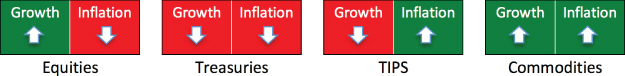
Figure 9.1 The Economic Bias of Four Major Asset Classes
Stocks and commodities tend to outperform when growth is rising; long-term Treasuries and TIPS do well when growth is falling; TIPS and commodities produce strong results when inflation is rising; and stocks and Treasuries do well when inflation is falling. Two of these four asset classes are biased to outperform in each of the four economic environments (rising/falling growth and inflation), as displayed in Table 9.1. This table shows the average return of each asset class since 1927, the type of environment in which it beat its average, and the climate in which it is favored to underperform its average (identified as good and bad environments, respectively). You have seen these numbers separated out before, but here they are presented side by side.
Table 9.1 Annualized Asset Class Excess Returns by Economic Environment (1927–2013)
| Asset Class | Average Excess Return for All Periods (Good and Bad) | Good Environment (Average Excess Return) | Bad Environment (Average Excess Return) |
| Equities | 5.6% | Rising growth (10.7%) | Rising inflation (1.9%) |
| Falling inflation (9.5%) | Falling growth (1.3%) | ||
| Long-Term Treasuries | 1.4% | Falling growth (5.5%) | Rising inflation (0.2%) |
| Falling inflation (2.6%) | Rising growth (−3.0%) | ||
| Long-Term TIPS | 4.6% | Rising inflation (10.7%) | Rising growth (1.1%) |
| Falling growth (7.9%) | Falling inflation (–1.1%) | ||
| Commodities | 2.0% | Rising inflation (8.4%) | Falling growth (–2.3%) |
| Rising growth (7.0%) | Falling inflation (–4.0%) |
Return of cash averaged 3.8 percent per year from 1927 to 2013. Thus, total returns can be approximated by adding 3.8 percent to the average excess returns provided above.
Notice the wide divergences in average returns during good and bad environments for each asset class. Since these economic climates represent about half of the total time period since 1927, the differences are meaningful.
Table 9.1 provides long-term averages. How about returns over longer cycles? Comparing the major long-term shifts in the economic environment over time to the impact on various asset class returns provides great insight into the bias of each asset class. Table 9.2 lists each major historical economic shift since 1927 and the best and worst asset class excess returns during that period. The data further corroborates the fact that changes in the economic climate largely explain fluctuations in asset class returns over longer time frames as well.
Table 9.2 Asset Class Returns during Major Economic Shifts (1927–2013)
| Economic Climate | Asset Class Annualized Excess Returns | |||
| Period | Growth | Inflation | Best | Worst |
| 1927–1929 | Rising | Falling | Equities +41.9% | TIPS –11.8% |
| 1929–1939 | Falling | Deflation | Treasuries +4.9% | Commodities –7.0% |
| 1939–1949 | Volatile | Rising | TIPS +15.6% | Treasuries +2.5% |
| 1949–1965 | Rising | Stable | Equities +13.4% | Treasuries –1.6% |
| 1965–1982 | Volatile | Rising | Commodities +5.8% | Treasuries –5.0% |
| 1982–2000 | Rising | Falling | Equities +12.7% | TIPS +1.5% |
| 2000–2013 | Falling | Stable | TIPS +9.6% | Equities/Commodities +1.2% |
Notice the change in the leaders and laggards during the various economic environments. The shifting economic climate predictably and reliably causes various asset classes to perform vastly different from their long-run averages during these extended periods. In each instance the actual economic outcome resulted in an asset class return that was consistent with what you would have expected given each class's underlying economic bias. Moreover, the cycles have been prolonged and have lasted for a decade or longer. Since one of our major goals in building a balanced portfolio is to minimize the risk of experiencing an extended period of underperformance, we should recognize how the economic environment is responsible for such an outcome.
I will make one final point before proceeding to the subject of how to think about weighting these four asset classes in your balanced portfolio. You may have noticed that cash was not included as one of the market segments offered above. Recall that we are trying to construct a balanced portfolio that is designed to capture the excess returns above cash over time while minimizing the variability around the average return.
There are environments during which cash is the best performing investment, outgaining all other market segments (often by not going down, while the rest temporarily lose money). Because of the completely divergent economic environmental bias of each of the four asset classes discussed here, it is quite rare that all four would simultaneously lose money. Regardless of whether the economy is strong or weak, or inflation is rising or falling, something is bound to perform well. Even during the extreme case of deflation, Treasury bonds will potentially outreturn cash.
The main reason cash is excluded is because over time it does worse than the other asset classes. This is because these asset classes offer positive excess returns above cash. You don't know what the economic environment will be in the future and how it will change course over time, but you do know that you can build a portfolio that by and large is immunized against these shifts.
Furthermore, the periods in which cash outperforms the other asset classes rarely occur, are short-lived, and are very difficult to anticipate in advance. Few, if any, have a successful long-term record of consistently accurately predicting when to hold cash over other asset classes. As a result, a constant allocation to cash merely lowers expected returns over time without providing much benefit. For this reason, it has been excluded as a viable asset class in the well-balanced portfolio.
Question Two: How Do I Weight the Asset Classes?
Now that you have selected asset classes that cover all the potential economic outcomes, the next step is to determine how much you should allocate to each. Let's start by looking at this from the highest level. The goal is to gain exposure to the shifts in the economic climate, since these shifts are largely responsible for the fluctuations of excess returns offered by asset classes. When one of these unpredictable shifts occurs, you want to make sure that your portfolio has sufficient exposure to that environment so that you benefit from its occurrence. Again, the goal is not to predict which environment will dominate next, but to position yourself so that you are by and large indifferent to what occurs. By exposure I am referring to the idea that the excess returns you capture from that environment are large enough to roughly offset underperformance in the rest of the portfolio, which is invested in market segments that were not favorably influenced by the economic environment that transpired.
In reality, they don't exactly offset each other so that the net result is zero. If that were the case, there would be no point in investing at all. Instead, the positives and negatives that I am talking about are related to average excess returns, which are all positive (rather than zero). In other words, a negative environment produces a below-average excess return and a positive climate generates an above-average excess return. For instance, if the average excess return for equities is 5.6 percent per year, then a slightly bad environment may lead to an excess return of 3.6 percent and a slightly good period 7.6 percent. Of course, a really bad economic climate would likely result in a negative excess return, but the baseline to which results should be compared is the average rather than zero. The same holds for each asset class, which has a positive average excess return.
You are trying to capture the excess returns offered by various asset classes over time while minimizing the volatility due to fluctuations of those excess returns. By neutralizing the impact of shifts in the economic environment, which is what mostly causes the fluctuation around average excess returns, you are able to roughly accrue the excess returns while minimizing volatility. Thus, the positives and negatives net out at some positive excess return above cash over time. Thus, when I refer to focusing on maintaining exposure to various economic climates such that the positives offset the negatives, it is to earn a positive excess return, rather than a zero excess return.
When thinking in terms of exposures, the analysis involves both the economic exposure as well as the return impact of the occurrence of each environment. It is not enough to say that you've covered all the environments and therefore have sufficient exposure to various economic outcomes. The returns during those various outcomes need to be considered as well. For instance, if you own bonds to protect against falling growth, but only own a 5 percent allocation, then when growth is falling this portfolio segment will not rise enough to offset negative excess returns elsewhere. You covered the exposure by owning the bonds, but you did not have sufficient coverage because you failed to own enough of the bonds (only 5 percent of your portfolio outperformed). It takes both parts to make it work effectively and to produce a well-balanced asset allocation.
You can achieve sufficient exposure by allocating more to a particular asset class. If stocks were prepackaged to offer you exposure to rising growth and falling inflation climates, then a higher allocation to stocks would naturally provide your portfolio with greater exposure to these environments. However, there is one other factor besides the weighting to the asset class that must be considered in this process.
The Impact of Volatility
A critical step in the conceptual process of allocating the assets is to factor in the volatility of the asset class. This is because the volatility also impacts the exposure provided by the asset class. Those asset classes that are highly volatile will fluctuate around their average more than those that are less volatile. The reason the volatility is the key step in the process is because it is this measure that specifically quantifies the fluctuations around the average excess return.
Your focus here should not be on precision but on the conceptual logic that follows. You do not need to calculate the exact volatility of an asset class and you do not need to worry about whether the volatility is higher or lower than normal. Keep the analysis very simple to ensure that you are grasping the concepts of why volatility is a key input in the determination of how to efficiently weight asset classes.
Ultimately, exposure comes from two factors: how much you own and the volatility of what you own. Consider an extreme example. The economic exposure of a 1-year Treasury bond and a 30-year Treasury bond is exactly the same. Both are biased to outperform during falling inflation and falling growth environments. For argument's sake, let's say the average excess return above cash for each is also similar. The key difference between these two is that the short-term bond will be reliably less volatile than the longer-dated security because of the significantly shorter duration of the former. What the higher volatility means is that the price of the long-term bond is going to fluctuate much more around its average return than that of the short-term bond. If you were to allocate 30 percent of your portfolio to 1-year bonds, then during falling inflation, falling growth climates, or both, the 1-year bond will likely outperform its average excess return. However (and this is the critical insight to appreciate), the 1-year bond's return during the favorable environment will not be much better than its return during other periods because it is not very volatile. Therefore, the real exposure (in terms of returns you will earn with this allocation) will not move very much. You have effectively covered two of the three parts of the key inputs. You gained exposure to the right environment, which provided a boost to your portfolio. You also allocated a healthy amount to the asset class, so you benefit from that move. However, since the segment in which you invested was not very volatile, the positive return was not very high and likely insufficient to properly balance your portfolio.
Conversely, the 30-year bonds are extremely volatile. The same allocation of 30 percent to this segment would provide much greater exposure to falling inflation and falling growth environments than a similar allocation to the short-term bonds. This is because during a positive environment for this asset class, the more volatile bonds are likely to produce a very high return for the same allocation. You will notice that another way to consider this is that a lower allocation to the longer-maturity bonds could be maintained to gain the same exposure as that provided by the less volatile bonds (which carries the additional benefit of leaving more money to invest elsewhere). Recall that the only difference between these two bond portfolios is that the volatility of one is much higher than that of the other. This logic may sound counterintuitive, but within this context higher volatility is superior to lower volatility.
Using this understanding, the conceptual logic of determining the appropriate weight to each asset class is to factor in both volatility and economic bias in the process. This is precisely the reason that long-term Treasuries and TIPS are being used for construction of a balanced portfolio rather than shorter-term bonds. Since the goal is to balance the risk of the asset classes, we want greater volatility from the typically low-volatility asset classes such as Treasuries and TIPS. The reason is simple: If the volatility of the bond segment is too low, then you would have to allocate a significant proportion of the portfolio to this asset to make up for its low volatility. This higher allocation would negatively impact your total expected return because bonds are a lower returning asset class. Thus, longer-duration bonds provide greater diversification benefits than do shorter-term (lower volatility) equivalent bonds because of how they fit within the balanced portfolio framework. Too little volatility in bonds prevents them from rising enough to protect the portfolio during environments in which the other, more volatile, asset classes underperform. Likewise, when bonds underperform there is enough volatility in the remaining asset classes to offset them, since the volatilities have been matched. The key is that the same environment that causes the bonds to underperform is likely to produce upside elsewhere.
Putting It Together
Now that we have selected a handful of asset classes that have different economic biases for our balanced portfolio, how should we think conceptually about constructing our asset allocation? We need to determine how much of each asset class needs to go into our total portfolio, as depicted in Figure 9.2.
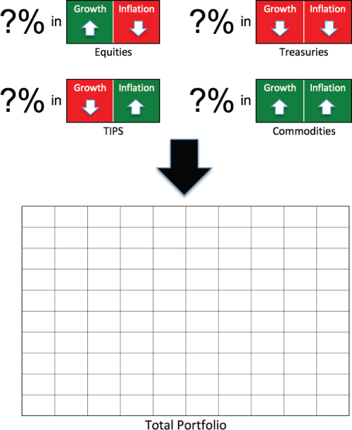
Figure 9.2 Weighting the Asset Classes
In Figure 9.2, the total portfolio is divided into 100 boxes. Each box represents a 1 percent position, or one unit. If we put one unit of equities into the portfolio, then 1 percent of the portfolio would consist of equities. Since we are thinking in terms of economic environmental biases, a portfolio of one unit of equities would have a slight bias toward rising growth and falling inflation (since 99 out of 100 boxes in the portfolio would have no bias). The total portfolio obviously takes on the economic biases of its parts. If we make the portfolio 100 percent equities, then it would be clearly biased to do well when growth is rising and when inflation is falling.
One way to visualize the impact of volatility using the asset class boxes is to adjust the number of arrows according to the asset's volatility. More volatile asset classes will have more arrows and less volatile classes will have fewer arrows. More arrows will indicate greater exposure to that particular economic environment.
To keep it simple, we can say that highly volatile assets can be marked with three arrows, medium-volatility with two, and low-volatility assets with just one arrow. Low volatility might have a standard deviation in the range of 4–6 percent, medium 8–12 percent, and high 14–20 percent. Notice that medium has about twice the volatility of low and high is about three times the volatility of low. The idea is to indicate the magnitude of the economic bias. The direction of the arrows doesn't change since the bias doesn't change, but the greater the volatility, the more significant the sensitivity to that particular environment. Consider the diagram in Figure 9.3, which tries to convey this important conceptual link.
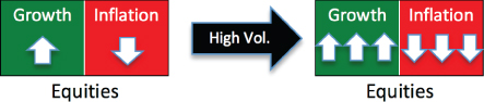
Figure 9.3 Factoring in Volatility: Equities
When the high volatility of equities is factored into the equation, the arrows for rising growth increase from one to three, as do the arrows for falling inflation. The direction of the arrows is not modified, but the greater number of arrows illustrates the magnitude of the environmental bias. If equities were medium volatility, there would only be two arrows in the rising-growth box and two in the falling-inflation box; if they were low volatility, there would just be one arrow in each box.
The difference is crucial from an exposure standpoint. Two units of a low-volatility asset class provide roughly the same exposure as one unit of a medium-volatility asset class, assuming both have the same environmental bias. Why is this? What really causes returns to fluctuate is the economic exposure. The more volatile an asset, the greater the variation between good and bad environments. Two units invested in low-volatility Treasuries provide roughly the same exposure to falling growth and falling inflation as one unit invested in medium-volatility Treasuries (assuming the volatility of the latter is twice that of the former). It is just like owning double the allocation from an economic exposure standpoint.
The same volatility adjustment can be made to the other asset classes, as shown in Figure 9.4.
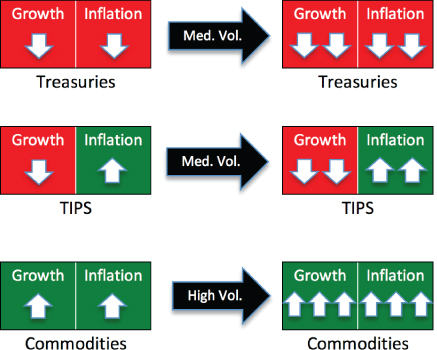
Figure 9.4 Factoring in Volatility: Treasuries, TIPS, and Commodities
The natural conclusion from the preceding thought sequence is that you either need to own more of the lower-volatility asset classes and less of the higher-volatility asset classes or somehow equalize the volatility of them all. This is an inevitable truth because otherwise the portfolio will simply not be economically balanced. And as I have emphasized, economic balance is crucial because it is the unpredictable shifting environment that by and large impacts asset class returns.
Although I am not espousing such a strategy in this book, you should know that you could roughly equalize the volatility of the asset classes by incorporating leverage. That is, you could take lower-volatility asset classes and use leverage to increase their volatilities to match the higher-volatility segments. To keep it simple, however, the emphasis in this book will be on extending duration in the more stable fixed income assets rather than incorporating leverage. Increasing the maturity of the bonds to longer-dated securities materially escalates their volatility. Either approach works; the key is to emphasize the core concepts behind building a balanced portfolio.
The bottom line is that this entire process is all about covering the various economic environments with equal exposure because these are what fundamentally and reliably drive asset class returns. Therefore, it is the volatility of each asset class that should be used to determine the appropriate weighting.
After adjusting each asset class that we are considering putting into our portfolio by its volatility, we are left with a picture that looks more like the one shown in Figure 9.5.

Figure 9.5 Weighting the Asset Classes: Factoring in Volatility
This figure more accurately illustrates the decision that needs to be made because it views each asset class with a complete summary of its total economic exposure. Importantly, this full depiction incorporates the asset class's volatility as well as its fundamental economic bias.
The final step in the process is to come up with a combination of asset classes so that the total portfolio's exposure to the various economic environments is neutral. Neutral in this case means that when you add up all the economic biases of the component asset classes you end up with totals that are roughly balanced. There should be about the same exposure to rising growth as there is to falling growth and the same for rising inflation as falling inflation.
If there were one (hypothetical) asset class that was not biased to outperform in rising/falling growth or rising/falling inflation environments, then you could simply construct a portfolio entirely made up of that single asset class to achieve this objective (assuming it also offers an attractive expected excess rate of return). However, since such an asset is not readily available, we have to construct a portfolio that consists of a mix of asset classes, each of which has different biases.
The trick is to decide how much of each asset class to insert into the portfolio so that it adds up to a neutral total portfolio that is not biased to outperform during any economic climate. This would represent a truly balanced portfolio with an efficient, neutral allocation. If you do not have strong feelings about a certain economic outcome, then a portfolio that is balanced and neutral would be an appropriate allocation. It can also serve as an efficient starting point if you do decide to tilt your allocation in favor of one outcome versus another.
From a conceptual standpoint, identifying a balanced mix is relatively straightforward using the illustrations provided. Simply add up the arrows in each environment. One unit (or 1 percent allocation) of equities means that you have three arrows in rising growth and three in falling inflation. By adding one unit of long-term Treasuries, you would then include two arrows in falling growth and two in falling inflation. A portfolio made up of 1 percent equities and 1 percent long-term Treasuries would then have three arrows in rising growth, two in falling growth, and five in falling inflation. This is not a well-balanced portfolio because it will likely do a little better during rising growth than falling growth (since it consists of three arrows in rising and two in falling growth). From an inflation standpoint, it is even less balanced. It will do very well during falling inflation and terribly during rising inflation since it owns no assets biased to the latter economic climate (as indicated by zero arrows for that environment). This process can be continued until you have filled up all 100 boxes in (or 100 percent of) the portfolio.
You can follow the same philosophy when you include other asset classes and can continue with this approach until you end up with a balanced mix. In the next chapter, I will provide step-by-step instructions to complete the asset allocation process. Before proceeding, however, it is important that you grasp the conceptual framework of what it really means for a portfolio to be well balanced. Whatever the process, the end result needs to produce a portfolio that is not biased to do better or worse during any of the various economic outcomes.
Summary
This is a very simplistic, yet effective conceptual approach to identifying balance in a portfolio. It is clearly not an exact science, but it doesn't have to be. It is the logical connections that are critical. The bias of each asset class to the various environments is reliable. The impact of volatility to this bias is reasonable. Combining the asset classes from an economic bias perspective makes sense since we want the total portfolio to be economically balanced. It really is that easy.