Chapter 15
Making Moves with Matrices
IN THIS CHAPTER
![]() Getting lined up with matrices
Getting lined up with matrices
![]() Operating on matrices
Operating on matrices
![]() Singling out single rows for operations
Singling out single rows for operations
![]() Identifying the inverses of matrices
Identifying the inverses of matrices
![]() Employing matrices to solve systems of equations
Employing matrices to solve systems of equations
A matrix is a rectangular array of numbers. It has the same number of elements in each of its rows, and each column shares the same number of elements. If you’ve seen the Matrix films, you may remember the lines and columns of green code scrolling down the characters’ computer screens. This matrix of codes represented the abstract “matrix” of the films. Putting numbers or elements in an orderly array allows you to organize information, access information quickly, do computations involving some of the entries in the matrix, and communicate your results efficiently.
 The word matrix is singular — you have just one of them. When you have more than one matrix, you have matrices, the plural form. Bet you weren’t expecting an English (or Latin) lesson in this book.
In this chapter, you discover how to add and subtract matrices, how to multiply matrices, and how to solve systems of equations by using matrices. The processes in this chapter are easily adaptable for use in technology (as evidenced by the machines in The Matrix!) — you can transfer the information to a spreadsheet, phone app, or graphing calculator for help with computing large amounts of data.
Describing the Different Types of Matrices
A matrix has a size, or dimension, that you have to recognize before you can proceed with any matrix operations.
 You give the dimensions of a matrix in a particular order. You identify the number of rows in the matrix first, and then you mention the number of columns. Usually, you put the numbers for the rows and columns on either side of
 ![]() :
: ![]() .
.
In the following list, you see six matrices. I’ve indicated their dimensions and some other classifications for several of them. You see more on the classifications in the next few sections. The brackets around the array of numbers serve as clear indicators that you’re dealing with matrices.
- Dimension
 :
: 
- Dimension
 (square matrix):
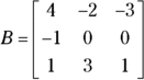
- Dimension
 (row matrix):
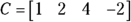
- Dimension
 (column matrix):
- Dimension
 (zero matrix):
- Dimension
 (square matrix, identity matrix):
 When you have to deal with more than one matrix, you can keep track of them by labeling the matrices with different names. You don’t call the matrices Bill or Ted; that wouldn’t be very mathematical of you! Matrices are traditionally labeled with capital letters, such as matrix A or matrix B, to avoid confusion.
The numbers that appear in the rectangular array of a matrix are called its elements. You refer to each element in a matrix by listing the same letter as the matrix’s name, in lowercase form, and following it with subscript numbers for the row and then the column. For example, the item in the first row and third column of matrix B is ![]() , which, in the matrix B shown here, is
, which, in the matrix B shown here, is ![]() . If the number of rows or columns grows to a number bigger than nine, you put a comma between the two numbers in the subscript.
. If the number of rows or columns grows to a number bigger than nine, you put a comma between the two numbers in the subscript.
Row and column matrices
Matrices come in many sizes (or dimensions), just like rectangles, but instead of measuring width and length, you count a matrix’s rows and columns. You call matrices that have only one row or one column row matrices or column matrices, respectively. A row matrix has the dimension ![]() , where n is the number of columns. The matrix C in the preceding section is a row matrix with dimension
, where n is the number of columns. The matrix C in the preceding section is a row matrix with dimension ![]() .
.
A column matrix has the dimension ![]() , where m is the number of rows. Matrix D from the previous section is a column matrix with dimension
, where m is the number of rows. Matrix D from the previous section is a column matrix with dimension ![]() .
.
Square matrices
A square matrix has the same number of rows and columns. Square matrices have dimensions such as ![]() ,
, ![]() ,
, ![]() , and so on. The elements in square matrices can take on any number — although some special square matrices have the label identity matrices (coming up later in this section). All matrices are rectangular arrays, and a square is a special type of rectangle. You see two square matrices in the earlier list. Both B and F are square matrices.
, and so on. The elements in square matrices can take on any number — although some special square matrices have the label identity matrices (coming up later in this section). All matrices are rectangular arrays, and a square is a special type of rectangle. You see two square matrices in the earlier list. Both B and F are square matrices.
Zero matrices
Zero matrices can have any dimension — they can have any number of rows or columns. The matrix E in the earlier listing is a zero matrix because zeros make up all the elements.
Zero matrices may not look very impressive — after all, they don’t have much in them — but they’re necessary for matrix arithmetic. Just like you need a zero to add and subtract numbers, you need zero matrices to do matrix addition and matrix subtraction.
Identity matrices
Identity matrices add a couple characteristics to the zero-matrix format (see the previous section) in terms of their dimensions and elements. An identity matrix has to
- Be a square matrix.
- Have a diagonal strip of 1s that goes from the top left to the bottom right of the matrix.
- Consist of zeros outside of the diagonal strip of 1s.
The matrix F in the earlier listing is an identity matrix, although you come across many, many more sizes — all square.
Identity matrices are instrumental to matrix multiplication and matrix inverses. Identity matrices act pretty much like the number one in the multiplication of numbers. What happens when you multiply a number times one? The number keeps its identity. You see the same behavior when you multiply a matrix by an identity matrix — the matrix stays the same.
Performing Operations on Matrices
You can add matrices, subtract one from another, multiply them by numbers, multiply them times each other, and divide them. Well, actually, you don’t divide matrices; you change the division problem to a multiplication problem. You can’t add, subtract, or multiply just any matrices, though. Each operation has its own set of rules. I cover the rules for addition, subtraction, and multiplication in this section. (Division comes later in the chapter, after I discuss matrix inverses.)
Adding and subtracting matrices
 To add or subtract matrices, you have to make sure the matrices are same size. In other words, they need to have identical dimensions. You find the resulting matrix by performing the operation on the corresponding elements in the matrices. If two matrices don’t have the same dimension, you can’t add or subtract them, and you can do nothing to fix the situation.
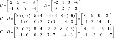
Here I show you two matrices and how their elements are added and subtracted.

You can see why matrices have to have the same dimensions before you can add or subtract. Differing matrices would have some elements without partners.
Here are some actual computations — adding and subtracting matrices C and D from the earlier section “Describing the Different Types of Matrices.” For each, you just add or subtract the corresponding elements:
Multiplying matrices by scalars
Scalar is just a fancy word for number. Algebra uses the word scalar with regard to matrix multiplication to contrast a number with a matrix, which has a dimension. A scalar has no dimension, so you can use it uniformly throughout the matrix.
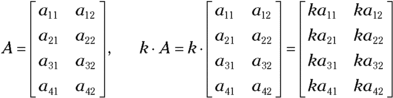
Scalar multiplication of a matrix signifies that you multiply every element in the matrix by a number.
To multiply matrix A by the number k, for example, you multiply each element in A by k. The matrix A and scalar k illustrates how this scalar multiplication works.
Here’s how the process looks with actual numbers. Multiplying the matrix F by the scalar 3, you create a matrix where every element is a multiple of 3:

Multiplying two matrices
Matrix multiplication requires that the number of columns in the first matrix is equal to the number of rows in the second matrix. This means, for instance, that a matrix with 3 rows and 11 columns can multiply a matrix with 11 rows and 4 columns — but it has to be in that order. The 11 columns in the first matrix must match up with the 11 rows in the second matrix.
Matrix multiplication requires some strict rules about the dimensions and the order in which the matrices are multiplied. Even when the matrices are square and can be multiplied in either order, you don’t get the same answer when multiplying them in the different orders. In general, the product AB does not equal the product BA.
Determining dimensions
If you want to multiply matrices, the number of columns in the first matrix has to equal the number of rows in the second matrix. After you multiply matrices, you get a whole new matrix that features the number of rows the first matrix had and the number of columns from the original second matrix. The process is sort of like cross-pollinating white and red petunias and getting pink.
In algebraic terms, if matrix A has the dimension ![]() and matrix B has the dimension
and matrix B has the dimension ![]() , to multiply
, to multiply ![]() , n must equal p. The dimension of the resulting matrix will be
, n must equal p. The dimension of the resulting matrix will be ![]() , the number of rows in the first matrix and the number of columns in the second.
, the number of rows in the first matrix and the number of columns in the second.
For example, if you multiply a ![]() matrix times a
matrix times a ![]() matrix, you get a
matrix, you get a ![]() matrix. However, you can’t multiply a
matrix. However, you can’t multiply a ![]() matrix by a
matrix by a ![]() matrix. Further emphasizing that the order in which you multiply the matrices does indeed matter, you can multiply a
matrix. Further emphasizing that the order in which you multiply the matrices does indeed matter, you can multiply a ![]() matrix by a
matrix by a ![]() matrix and get a
matrix and get a ![]() matrix.
matrix.
Defining the process
Multiplying matrices is no easy matter, but it isn’t all that difficult — if you can multiply and add correctly. When you multiply two matrices, you compute the elements with the following rule:
If you find the element ![]() after multiplying matrix A times matrix B,
after multiplying matrix A times matrix B, ![]() is the sum of the products of the elements in the ith row of matrix A and the jth column of matrix B.
is the sum of the products of the elements in the ith row of matrix A and the jth column of matrix B.
Okay, so that rule may sound like a lot of hocus pocus. How about I give you something a bit more concrete? Here’s a matrix A that has the dimension ![]() and a matrix B with the dimension
and a matrix B with the dimension ![]() . According to the rules that govern multiplying matrices, you can multiply A times B because the number of columns in matrix A is two, and the number of rows in matrix B is two. The matrix that you create when multiplying A and B has the dimension
. According to the rules that govern multiplying matrices, you can multiply A times B because the number of columns in matrix A is two, and the number of rows in matrix B is two. The matrix that you create when multiplying A and B has the dimension ![]() .
.
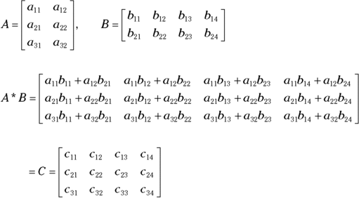
You find the element ![]() by multiplying the elements in the first row of A times the elements in the first column of B and then adding the products:
by multiplying the elements in the first row of A times the elements in the first column of B and then adding the products: ![]() . You find
. You find ![]() by multiplying the second row of matrix A times the third column of matrix B and adding:
by multiplying the second row of matrix A times the third column of matrix B and adding: ![]() .
.
Although the last example was more concrete, it didn’t provide you with numbers. With the following matrices, you can multiply matrix J times matrix K because the number of columns in matrix J matches the number of rows in matrix K. You can also see the computations needed to find the resulting matrix.
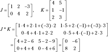
You get a ![]() matrix when you multiply because multiplying a
matrix when you multiply because multiplying a ![]() matrix times a
matrix times a ![]() matrix leaves you with two rows and two columns. The multiplication process may seem a bit complicated, but after you get the hang of it, you can do the multiplication and addition in your head.
matrix leaves you with two rows and two columns. The multiplication process may seem a bit complicated, but after you get the hang of it, you can do the multiplication and addition in your head.
Applying matrices and operations
One of the grand features of matrices is their capacity to organize information and make it more useful. If you’re running a small business, you can keep track of sales and payroll without having to resort to matrices. But big companies and factories have hundreds, if not thousands, of items to keep track of. Matrices help with the organization, and, because you can enter them in computers, the accuracy and ease of using them increases even more.
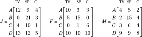
Consider the following sales situation that occurred in an electronics store where Avery, Ben, Carlie, and Don work. In January, Avery sold 12 televisions, 9 smartphones, and 4 computers; Ben sold 21 smartphones, and 3 computers; Carlie sold 4 TVs, 10 smartphones, and 1 computer; and Don sold 13 TVs, 12 smartphones, and 5 computers. Using the matrices J, F, and M, you see the sales results for Avery, Ben, Carlie, and Don during the month of January (you also see the sales for February and March). See how nicely the matrices organize the information!
When you organize the information into matrices, you can see at a glance who’s selling the most, who’s had some bad months, who’s had some good months, and what electronics seem to be moving the best. With this information in hand, several questions may come to mind.
Determining how many of each item was sold
The first question is: How many TVs, smartphones, and computers did the store sell during those three months? Because all the matrices J, F, and M have the same dimensions, you can add them together (see the section “Adding and subtracting matrices”). I next show you how you find the sales for the first three months of the year by adding the matrices (the totals of the individual salespeople).

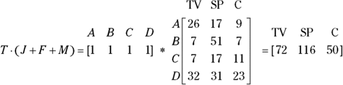
The way to use matrices to find the total sales for each type of electronic, you multiply the sum matrix (the matrix you just found) by a row matrix, ![]() . You’re multiplying a matrix with the dimension
. You’re multiplying a matrix with the dimension ![]() times a matrix with the dimension
times a matrix with the dimension ![]() , so your result is a matrix with the dimension
, so your result is a matrix with the dimension ![]() ; the totals of each electronic appear in order from left to right. Think of the row matrix T with the salespersons’ names across the top. When you multiply this matrix by the sum matrix, you match each of the columns in T with each of the rows in the sum. The columns in T and the rows in the sum are the salespersons, so they line up. By multiplying all the numbers in the second matrix by 1’s, you essentially multiply by 100 percent — you add everything up. The resulting matrix is a row matrix with the numbers for the electronics in the respective columns. First, the matrix T with its labels for each element is given by
; the totals of each electronic appear in order from left to right. Think of the row matrix T with the salespersons’ names across the top. When you multiply this matrix by the sum matrix, you match each of the columns in T with each of the rows in the sum. The columns in T and the rows in the sum are the salespersons, so they line up. By multiplying all the numbers in the second matrix by 1’s, you essentially multiply by 100 percent — you add everything up. The resulting matrix is a row matrix with the numbers for the electronics in the respective columns. First, the matrix T with its labels for each element is given by
And the following shows the computation and result.
You’re wondering why you can’t just add the numbers in each column, aren’t you? Go right ahead! That works, too. I show you this process with a small, reasonable number of items so you can see how you can instruct a computer to do it with hundreds or thousands of entries. You may also want to “weight” some entries — make some items worth more than others — if you’re keeping track of points. The row matrix can have different entries that align with the different items.
Determining sales by salesperson
Here’s another question you can answer with the matrix sum ![]() : How much money did each salesperson bring in? For instance, assume that the average costs of a TV, smartphone, and computer are $1,500, $400, and $2,000, respectively. You can construct a column matrix containing these dollar amounts, call it the dollar matrix, and multiply it by the sum matrix
: How much money did each salesperson bring in? For instance, assume that the average costs of a TV, smartphone, and computer are $1,500, $400, and $2,000, respectively. You can construct a column matrix containing these dollar amounts, call it the dollar matrix, and multiply it by the sum matrix ![]() .
.
The following matrix multiplication shows the multiplication of the sum matrix times the dollar matrix, with the resulting amount of money brought in by each salesperson.
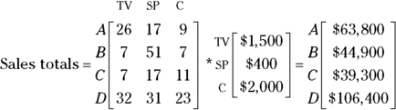
Here are the results of multiplying the entries in the row of the first matrix by the columns of the second:
- A:

- B:

- C:

- D:

Determining how to increase sales
Here’s one last question that deals with a percentage: How many electronic devices in each category must each salesperson sell if they have to increase sales to 125 percent during the next quarter?
You identify this problem as a scalar multiplication problem (see the section “Multiplying matrices by scalars”) because you multiply each entry in the sum matrix ![]() by 125 percent to get the sales target. The value 1.25 represents 125 percent — 25 percent more than the last quarter. This next computation shows the result of the scalar multiplication and a second matrix with the numbers rounded up. (You can’t sell half a computer, and rounding up gives the salesperson the number he or she needs to make or exceed the goal [not come in slightly below].)
by 125 percent to get the sales target. The value 1.25 represents 125 percent — 25 percent more than the last quarter. This next computation shows the result of the scalar multiplication and a second matrix with the numbers rounded up. (You can’t sell half a computer, and rounding up gives the salesperson the number he or she needs to make or exceed the goal [not come in slightly below].)

Defining Row Operations
Along with the matrix operations I list in the previous sections of this chapter, you can perform row operations on the individual rows of a matrix. You perform a row operation one matrix at a time; you don’t combine one matrix with another matrix when performing these operations. A row operation changes the look of a matrix by altering some of the elements, but proper operations allow the matrix to retain the properties that enable you to use it in other applications, such as solving systems of equations. (See the section “Using Matrices to Find Solutions for Systems of Equations” later in this chapter.)
The business of changing matrices to equivalent matrices is sort of like changing fractions to equivalent fractions so they have a common denominator — the change makes the fractions more useful. The same goes for matrices.
You have several different row operations at your disposal:
- You can exchange two rows.
- You can multiply the elements in a row by a constant (not zero).
- You can add the elements in one row to the elements in another row.
- You can add a row that you multiply by some number to another row.
Next I show you a matrix that has experienced the following row operations, in order, each on the previous result. I use a special notation or shorthand to indicate what operations are being performed (it’s the one I introduce in Chapter 12 when performing operations on linear equations):
- a: I exchange the first and third rows, indicated by
 .
. - b: I multiply the second row through by
 , indicated with
  .
. - c: I add the first and third rows and put the result in the third row, shown with
 .
. - d: I add twice the first row to the second row and put the result in the second row, shown by
 .
.

Performing row operations correctly results in a matrix that’s equivalent to the original matrix. The rows themselves aren’t equivalent to one another; the whole matrix and the relationships between its rows are preserved with the operations.
Row operations may seem pointless and aimless. For these illustrations of the row, I have no particular goal other than to illustrate the possibilities. But you choose more wisely when you do row operations to perform a task, such as solving for an inverse matrix (see the following section).
Finding Inverse Matrices
Inverses of matrices act somewhat like inverses of numbers. The additive inverse of a number is what you have to add to the number to get zero. For example, the additive inverse of the number 2 is ![]() , and the additive inverse of
, and the additive inverse of ![]() is 3.14159. Simple enough.
is 3.14159. Simple enough.
Algebra also provides you with the multiplicative inverse. Multiplicative inverses give you the number one. For example, the multiplicative inverse of 2 is ![]() .
.
Adding or multiplying inverses always gives you the identity element for a particular operation. Before you can find inverses of matrices, you need to understand identities, so I cover those in detail here.
Determining additive inverses
You can label the number zero as the additive identity, because adding zero to a number allows that number to keep its identity. The additive identity for matrices is a zero matrix. When you add a zero matrix to any matrix with the same dimension, the original matrix doesn’t change.
Inverse matrices associated with addition are easy to spot and easy to create. The additive inverse of a matrix is another matrix with the same dimension, but every element has the opposite sign. When you add the matrix and its additive inverse, the sums of the corresponding elements are all zero, and you have a zero matrix — the additive identity for matrices (see the section “Zero matrices” earlier in the chapter). The following matrix computation shows you how two matrices can add to nothing.

All matrices have additive inverses — no matter what the dimension of the matrix. This isn’t the case with multiplicative inverses of matrices. Some matrices have multiplicative inverses and some do not. Read on if you’re intrigued by this situation (or if the topic will be on your next test).
Determining multiplicative inverses
You can label the number 1 as the multiplicative identity, because multiplying a number by one doesn’t change the number — it keeps its identity.
Matrices have additive identities that consist of nothing but zeros, but multiplicative identities for matrices are a bit more picky. A multiplicative identity for a matrix has to be a square matrix, and this square matrix has to have a diagonal of ones; the rest of the elements are zeros. This arrangement assures that when you multiply any matrix times a multiplicative identity, you don’t change the original matrix. Here is the process of multiplying two different matrices by identities — one with the identity first and the other with it last. The multiplication rule for matrices still holds here (see the section “Multiplying two matrices”): The number of columns in the first matrix must match the number of rows in the second matrix.
The identity first:
And the identity last:

Like the multiplicative identity of a matrix, the multiplicative inverse of a matrix isn’t quite as accommodating as its additive cousin. When you multiply two matrices, you perform plenty of multiplication and addition, and you see plenty of change in dimension. Because of this, matrices and their inverses are always square matrices; non-square matrices don’t have multiplicative inverses.
If matrix A and matrix ![]() are multiplicative inverses,
are multiplicative inverses, ![]() , and
, and ![]() . The superscript
. The superscript ![]() on matrix A identifies it as the inverse matrix of A — it isn’t a reciprocal, which the exponent
on matrix A identifies it as the inverse matrix of A — it isn’t a reciprocal, which the exponent ![]() usually represents. Also, the capital letter I identifies the identity matrix associated with these matrices — with dimensions
usually represents. Also, the capital letter I identifies the identity matrix associated with these matrices — with dimensions ![]() ,
, ![]() ,
, ![]() , and so on.
, and so on.
Next, I multiply matrix B and its inverse ![]() in one order and then in the other order; the process results in the identity matrix both times.
in one order and then in the other order; the process results in the identity matrix both times.

Not all square matrices have inverses. But, for those that do, you have a way to find the inverse matrices. You don’t always know ahead of time which matrices will fail you, but it becomes apparent as you go through the steps. The first process, or algorithm (a process or routine that produces a result), you can use works for any size square matrix. You can also use a neat, quick method that’s special for ![]() matrices and works only for matrices with that dimension.
matrices and works only for matrices with that dimension.
Identifying an inverse for any size square matrix
The general method you use to find a matrix’s inverse involves writing down the matrix, inserting an identity matrix, and then changing the original matrix into an identity matrix.
To solve for the inverse of a matrix, follow these steps:
- Create a double matrix — consisting of the target matrix and the identity matrix of the same size — with the identity matrix to the right of the original.
Perform row operations until the elements on the left become an identity matrix (see the “Defining Row Operations” section earlier in the chapter).
The elements created in the new left-hand matrix need to feature a diagonal of ones, with zeros above and below the ones. Upon completion of this step, the elements on the right become the elements of the inverse matrix.
For example, say you want to solve for the inverse of matrix M in the following figure. You first put the ![]() identity matrix to the right of the elements in matrix M. The goal is to make the elements on the left look like an identity matrix by using matrix row operations.
identity matrix to the right of the elements in matrix M. The goal is to make the elements on the left look like an identity matrix by using matrix row operations.

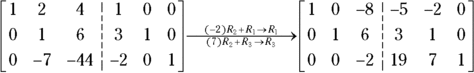
The identity matrix has a diagonal slash of ones, and zeros lie above and below the ones. The first thing you do to create your identity matrix is to get the zeros below the one in the upper left-hand corner of the original identity. Here are the row operations you use for this example:
- Multiply Row 1 times 3 and add the result to Row 2, making the result the new Row 2.
- Multiply Row 1 by
 and add the result to Row 3, putting the resulting answer in Row 3.
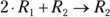
The following shows what the matrix looks like after you perform the row operations. The notation on the arrow between the two matrices describes the row operations you use.

You see a one in the second column and second row of the resulting matrix — along the diagonal of ones that you want. Getting the one in this position is a nice coincidence; it doesn’t always work out as well. If the one hadn’t fallen in that position, you’d have to divide the whole row by whatever number makes that element a one.
Now, you want zeros above and below the 1 in the middle, so you follow these steps:
- Multiply Row 2 by
 and add the result to Row 1.
 - Multiply Row 2 by 7 and add the result to Row 3.
You now need to turn the element in the third row, third column of the matrix into a 1, so you multiply the row through by ![]() ; this multiplication is the same as dividing through by
; this multiplication is the same as dividing through by ![]() .
.

You have one last set of row operations to perform to get zeros above the last one on the diagonal:
- Multiply Row 3 by 8 and add the elements in the row to Row 1.
- Multiply Row 3 by
 and add the result to Row 2.
The following shows the final two steps and the result.
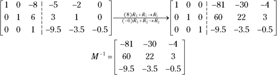
The operations gave you a ![]() identity matrix on the left and a new
identity matrix on the left and a new ![]() matrix on the right. The elements in the matrix on the right form the inverse matrix,
matrix on the right. The elements in the matrix on the right form the inverse matrix, ![]() . The product of M and its inverse,
. The product of M and its inverse, ![]() , is the identity matrix.
, is the identity matrix.
The following checks your work — showing that ![]() is the identity matrix:
is the identity matrix:

How can you tell when a matrix doesn’t have an inverse? You can’t get ones along the diagonal by using the row operations. You usually get a whole row of zeros as a result of your row operations. A row of zeros is the warning that no inverse is possible.
Using a quick-and-slick rule for 2 × 2 matrices
You have a special rule at your disposal to find inverses of ![]() matrices. To implement the rule for a
matrices. To implement the rule for a ![]() matrix, you have to switch two elements, negate two elements, and divide all the elements by the difference of the cross products of the elements. This may sound complicated, but the math is really neat and sweet, and the process is much quicker than the general method (see the previous section).
matrix, you have to switch two elements, negate two elements, and divide all the elements by the difference of the cross products of the elements. This may sound complicated, but the math is really neat and sweet, and the process is much quicker than the general method (see the previous section).
Here is the general formula for the ![]() matrix rule.
matrix rule.
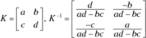
As you can see from this special rule, the upper-left and lower-right corner elements are switched; the upper-right corner and lower-left corner elements are negated (changed to the opposite sign); and all the elements are divided by the result of doing two cross products and subtracting.
To find the inverse of matrix Z using the ![]() method, you switch the 5 and the 11, you change the 6 to
method, you switch the 5 and the 11, you change the 6 to ![]() and the 9 to
and the 9 to ![]() , and you divide by the difference of the cross products:
, and you divide by the difference of the cross products: ![]() . Watch the order in which you do the subtraction — the order does matter. Dividing each element by 1 doesn’t change the elements, as you can see.
. Watch the order in which you do the subtraction — the order does matter. Dividing each element by 1 doesn’t change the elements, as you can see.
Dividing Matrices by Using Inverses
Until this point in the chapter, I’ve avoided the topic of division of matrices. I haven’t spent much time on the topic because you don’t really divide matrices — you multiply one matrix by the inverse of the other (see the previous section for info on inverses). The division process resembles what you can do with real numbers. Instead of dividing 27 by 2, for example, you can multiply 27 by 2’s inverse, ![]() .
.
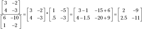
To perform matrix division on the matrix

you first find the inverse of the matrix in the denominator.

You then multiply the matrix in the numerator by the inverse of the matrix in the denominator (see the section “Multiplying two matrices” earlier in this chapter).
Using Matrices to Find Solutions for Systems of Equations
One of the nicest applications of matrices is that you can use them to solve systems of linear equations. In Chapter 12, you find out how to solve systems of two, three, four, and more linear equations. The methods you use in that chapter involve elimination of variables and substitution. When you use matrices, you deal only with the coefficients of the variables in the problem. This way is less messy, and you can enter the matrices into graphing calculators or computer programs for an even more relaxing process.
This method using matrices is the most desirable when you have some technology available to you. Finding inverse matrices can be nasty work if fractions and decimals crop up. Simple graphing calculators can make the process quite nice.
You can use matrices to solve systems of linear equations as long as the number of equations and variables is the same. To solve a system, adhere to the following steps:
Make sure all the variables in the equations appear in the same order.
Replace any missing variables with zeros, and write all the variable terms on one side set equal to the constant term.
- Create a square coefficient matrix, A, by using the coefficients of the variables.
- Create a column constant matrix, B, by using the constants in the equations.
Find the inverse of the coefficient matrix,
 .
.You can perform this step by using the procedures shown in the section “Finding Inverse Matrices” or by using a graphing calculator.
Multiply the inverse of the coefficient matrix times the constant matrix —
 .
.The resulting column matrix has the solutions, or the values of the variables, in order from top to bottom.
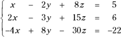
Say, for example, that you want to solve the following system of equations:
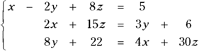
You first rewrite the equations so that the variables appear in order and the constants appear on the right side of the equations:
Now you follow Steps 2 and 3 by writing in the coefficient matrix, A, and the constant matrix, B (shown in the following figure):

Step 4 is finding the inverse of matrix A. Follow these steps:
- Write the identity matrix next to the original matrix.
- Add Row 2 to
 for a new Row 2, written
 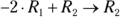 .
. - Add Row 3 to
 for a new Row 3, written
  .
. - Add Row 1 to
 for a new Row 1, written
  .
. - Multiply Row 3 by 0.5, written
 .
. - Add Row 1 to
 for a new Row 1, written
  .
. - Add Row 2 to Row 3 for a new Row 2, written
 .
.
Voila! The inverse matrix. See the following for the finished product:

Now you multiply the inverse of matrix A times the constant matrix, B (see the section “Multiplying two matrices”); you get a column matrix with all the solutions of x, y, and z listed in order from top to bottom:
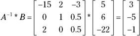
The column matrix tells you that ![]() ,
, ![]() , and
, and ![]() .
.