
CHAPTER
9
Tuning by Tier: The Database Tier (Microsoft SQL Server and IBM System i)
In this chapter we will discuss processes you can utilize to tune your Microsoft SQL Server and IBM System i databases. We will share some different strategies involved, since there are differences regarding how the databases relate to their operating systems. The Oracle database supported by EnterpriseOne can run on multiple platforms, such as Unix, Linux, and Microsoft Windows. For EnterpriseOne, Microsoft SQL Server operates only on the Microsoft Windows platform. IBM System i is even more integrated where the DB2/400 database is included in the operating system.
NOTE
A number of the monitoring and metric procedures discussed in this chapter are similar to those provided in Chapter 8. To minimize duplication of certain suggestions, please read Chapter 8 as well as this chapter, even though you may not be using an Oracle Database system. There are definitely a number of common areas regarding the EnterpriseOne databases, and we are attempting to provide some of the key tuning elements for each of those database systems. |
Tuning Microsoft SQL Server
With Microsoft SQL Server, it’s important that you maintain patch levels, ensure that you size and architect the database server appropriately, and perform a number of tuning options, as described here. Microsoft SQL Server 64-bit addressing provides great scalability and opportunities for JD Edwards EnterpriseOne; the 64 bit/x64 Microsoft SQL Server releases are the only supported levels now. Considering the use of database and backup compression along with Read Committed Snapshot Isolation (RCSI) can further enhance your system’s capabilities and resource usage.
Reviewing the Logs
This is one of the obvious and sometimes neglected tuning tasks, but we often find a number of clues in the various database, EnterpriseOne, and operating system logs. If you are experiencing performance issues, you need to ensure that the various logs have been reviewed. A number of general issues can occur due to application, resource, network, and other areas, even when someone “thinks” it is a database problem. We have often heard users blame “the network” or “the database” when the root cause was entirely different. Generally, administrators have access to behind-the-scenes logs of the processes, so we will focus on those. Error messages reported by the end user should generally be captured in a screenshot where possible and investigated to see if they can be linked to specific events in the various logs.
SQL Server Support: 32-bit vs. 64-bit
JD Edwards OneWorld and EnterpriseOne have supported Microsoft SQL Server since the introduction of the software. Historically, Microsoft SQL Server was ideal for Windows-based customers with smaller installations due to the use of 32-bit operating systems. Enhancements over the years provided additional memory and scaling with the use of Physical Address Extension (PAE) memory and Address Windowing Extensions (AWE). Unfortunately, these settings were sometimes implemented incorrectly, and the memory above the 32-bit address line was not utilized correctly. In addition, some other memory settings for 32-bit Windows, such as the /3GB switch, are no longer needed in the newer operating system releases that operate in 64-bit mode. With the introduction of Microsoft SQL Server 2005, 2008, and 2012, the use of 64-bit database memory access is the preferred and recommended requirement for EnterpriseOne releases. You no longer have to be concerned with 32-bit memory address space limitations, and this helps reduce some of the performance and tuning challenges of the past. Our advanced tuning focus is on the 64-bit/x64 Microsoft SQL Server releases, even though a portion of these suggestions can apply to older releases as well.
Microsoft SQL Server Logs
The Microsoft SQL Server logs can sometimes provide insights into the overall database activity if an error or warning occurs. A number of diagnostic tidbits can help you ascertain the release, patch level, configuration, and other information near the top of the log. If there are specific issues, such as a transaction log filling up, these are recorded here as well. This is an operational issue and not really tuning per se, but since all database activities that need to perform a data change halt until the log is cleared, it is a good first place to examine.
You can examine the SQL Server logs from the ERRORLOG text file, where the SQL Server instance is installed under the log folder. By default, for a 64-bit installation, this is C:Program FilesMicrosoft SQL ServerMSSQLxx.instancenameMSSQLLog folder. Or, if you have administrative access, use the Microsoft SQL Server Management Studio application to view the log files. An example is shown in the following illustration.
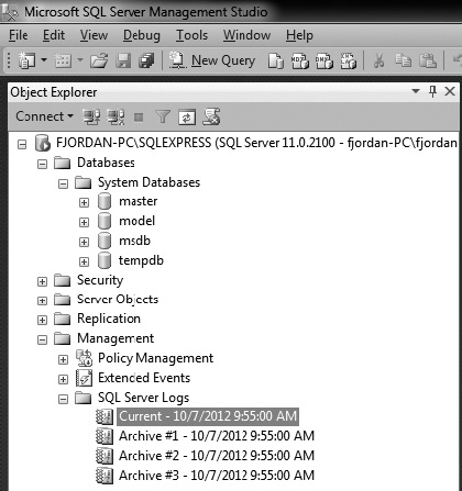
In the log, you can observe a number of informational items and the initial Microsoft SQL Server configuration. These can be very helpful in understanding the configuration of the system and what errors may be present.
Microsoft Windows Operating System Logs
The Microsoft Windows OS logs are used in a number of areas. The primary logs that we tend to investigate are the Windows Application, Security, and System Event logs. There are others depending how the server is configured, such as the Windows Firewall, file backup, or anti-virus logs.
Following are examples of what you may be searching for:
JD Edwards EnterpriseOne Logs
Most JD Edwards EnterpriseOne Configurable Network Computing (CNC) administrators and developers are familiar with the various logs that are created by EnterpriseOne processes/services. In Chapter 8, we referred to a number of the areas to review, such as utilizing EnterpriseOne Server Manager as a launch point to obtain details about the various components that access the Microsoft SQL Server database.
Following are examples of what you may be searching for:
Showing the SQL Statements in EnterpriseOne Server Logs
The following JDE.INI setting was introduced as part of the Kernel Resource Management (KRM) initiative in the Tools 8.98.3 release and provides a methodology by which SQL statements can be logged to the JDE logs if they exceed a time threshold. The JDE.INI setting is
This functionality is turned OFF when set to 0 and only positive integer values are valid for its usage. Set the
QueryExecutionTimeThreshold to 1 second to track any SQL statements that take more than 1 second to complete. This setting is read by EnterpriseOne services at startup and will require a restart of services to use if implemented. In the case of batch processing, the value is picked up when the batch process is launched, so it must be set prior to launching the batch process to have an effect. (Reference: http://docs.oracle.com/cd/E17984_01/doc.898/e14718.pdf.)Operating System/Database Patches
It is generally recommended that, where possible, you maintain the patch levels of your Windows OS and SQL Server. Different companies have various change management strategies, but we typically recommend that you attempt to keep the patch levels fairly current within 12 to 18 months if possible. This also applies to JD Edwards EnterpriseOne tools and software updates. If you allow the patch levels to become too out of date, it becomes more difficult to apply one-off or specific fixes over time due to increased dependency chains in the software. Also, from a support perspective, if your patches are out of date, it becomes more of a challenge for the software vendor to help resolve issues when the latest set of fixes that address known issues are not in place.
Every customer has different thresholds and philosophies regarding how they manage their patches. Very large customers with high levels of customization tend to apply patches at intervals of up to several years, while a number of smaller to midsize customers tend to be more current on their various patch levels. Another influencing factor can be government regulations and qualifications that limit the changes that can be introduced into the systems.
A general strategy employed during installations or upgrades is to attempt to update the software as frequently as possible before full integration tests occur. This helps to keep the patch levels more current and can indirectly influence the performance, since most patches are issued to correct functionality, memory, or performance issues. Once the various go-live phases are near the 30- to 90-day range, the patch levels tend to be stabilized and frozen until the next change window is reached that the business can tolerate. After the production environment goes live, we generally like to see security patches deployed monthly, database cumulative patches when needed, and Microsoft Windows/database service packs when certified by EnterpriseOne minimum technical requirements (MTRs) and your company is comfortable implementing them. Generally, this is a 12- to 24-month window and helps to reduce support challenges and apply corrections for known issues.
Keep in mind that the JD Edwards EnterpriseOne MTRs or certifications will also tend to influence the combination of Windows OS and SQL Server patch levels. If you update a Tools release level that is several years old, you typically need to examine newer Windows versions since the older releases most likely are near the end of their support life. For example, SQL Server releases typically occur every 3 to 5 years, so a newer JD Edwards EnterpriseOne tools release (9.1.x) may no longer be certified against a database level such as SQL Server 2005 x64 64-bit.
NOTE
A good Oracle Metalink document for EnterpriseOne Microsoft SQL Server customers is Document ID 1275500.1, “Tips for Running EnterpriseOne with SQL Server 2008 and SQL Server 2008 R2.” This document contains several suggestions that can help an EnterpriseOne customer’s architecture, which we also endorse and allude to in this guide. If we don’t mention certain tips, that does not mean they are not recommended, but from the advanced tuning perspective, we assume those areas are or have been reviewed and addressed. |
For the Windows OS, you should consider various strategies of patching. Examples are provided in Table 9-1.

TABLE 9-1. Windows OS Patch Types
The SQL Server databases also utilize similar patching strategies, as shown in Table 9-2.

TABLE 9-2. SQL Server Patch Types
TIP
At the Windows OS level, the server admins will most likely need critical security updates to be applied, so these need to be considered. You can use those planned outage windows for other patch updates for the OS and database as well if desired. If at all possible, try to define a least a monthly maintenance window, depending on the architecture in place. The grid architectures discussed in other chapters would allow you to service a subset of servers in a planned fashion without observed outages until you fail-over the database cluster. |
Always remember to review and operate within the JD Edwards EnterpriseOne MTRs/certifications for your Windows and SQL Server database configuration. Most customers adhere to the MTRs, which allows them to obtain support more readily. When the configuration becomes very old and back-leveled, it can become more of a challenge to tune or obtain patches since you may not receive support from the vendor. Since most vendors maintain their software for 5 years or longer, this may not be an issue, but we have observed some customers running software levels beyond 10 years, and it takes time to investigate and determine the best course of action when tuning or changing the configuration.
Microsoft SQL Server Service Account Privileges/Permissions
Most of the account policies and privileges for the SQL Server services are created during the database install into local user groups. This process began in SQL Server 2005 and later releases. (If you are still using SQL Server 2000, either upgrade or you will need to consult with older Microsoft Knowledge Base articles outside the scope of this book.) If you decide to use a domain or another user account, you simply add it to the appropriate local SQL Server group for that particular database instance. Some example privileges are SeBatchLogonRight, SeAssignPrimaryTokenPrivilege, and SeServiceLogonRight, among others.
The local user groups would have the format for SQL Server 2005, as shown here:
You’ll find a Microsoft Knowledge Base article listing the various SQL Server versions at http://msdn.microsoft.com/en-us/library/ms143504.aspx. You can select your database version and review the various permissions and account options available. Most EnterpriseOne customers that we have observed have a local account defined, and some utilize a domain user. There is no one-strategy-fits-all recommendation here; it is dependent on your infrastructure requirements.
Later, in the “Memory” section, we will discuss memory recommendations to consider such as using the Lock Pages in Memory (LPIM) and user rights on the SQL Server startup account. This recommendation is for all SQL Server releases, even though the memory management in Windows 2008 Server has improved substantially regarding hard trim working sets. Based on our consulting experience and observations, you can still have unintended performance issues with SQL Server being paged out at undesired rates. You can mitigate this by ensuring that the minimum and maximum SQL Server memory is set appropriately for your configuration.
SQL Server CPU, Memory, Network, and Disk Configuration
SQL Server performance is greatly influenced by the hardware configuration. The database is very scalable, with several editions from which the user can select. For JD Edwards EnterpriseOne Tools 9.1 and later, the SQL Server 2008/2008 R2 editions supported are the 64-bit x64 Standard, Enterprise, and Datacenter editions. Most customers above 50–100 users tend to utilize the Enterprise edition for maximum flexibility and features. At the time of this writing, the SQL Server 2012 editions supported by JD Edwards EnterpriseOne have not been announced. The lighter SQL Server Express (SSE) that was previously an option for the JD Edwards EnterpriseOne Windows development client and deployment server is no longer supported, beginning with EnterpriseOne 9.1 applications release.
You should have a very good understanding of your projected business needs for the test and production environments using SQL Server databases. The use of 64-bit addressing provides a very scalable database architecture that can be used for dozens to thousands of JD EnterpriseOne users. As we have stated, if you can obtain a sizing from your hardware vendor with accurate information, your architecture should meet your business needs. It is strongly recommended that you conduct performance and scaling tests before a go-live to ensure your architecture does meet those objectives.
When procuring hardware for your SQL Server database, we typically recommend that you obtain the most robust configuration that your budget will allow. This may seem to be a bit obvious, but typically hardware and software investment tends to be a low percentage of the overall project/implementation budget. The infrastructure costs almost always tend to be much less than the costs and effort involved with upgrading and implementing your JD Edwards EnterpriseOne and associated components solution.
TIP
It is usually very beneficial to obtain a JD Edwards EnterpriseOne sizing from your hardware vendor. Then, once the majority of business processes have been configured, you can examine the sizing again to ensure that your system meets the requirements before moving to a production environment. Common sense, we know, but this seems to have been ignored by a number of customers we’ve worked with over the years. If this is ignored, it usually becomes a consulting opportunity that typically occurs near or shortly after a go-live, which creates some grief and frustration for the business. This is an obvious, but often neglected task, and we strongly suggest conducting performance and scaling exercises. This has been emphasized in other chapters as well to drive the point home. |
The common items that have a relationship with and affect database tuning efforts are shown in Table 9-3. Generally, you will need to strike a balance between these elements, because if any of them are oversubscribed or saturated, this will affect the other areas. The basic goal we strive for is to ensure that each component is optimized on the server and using the various Microsoft performance tools such as Performance Data Collector, Performance Monitor, Task Manager, Resource Monitor, and DMVs, which allow you to observe the behavior of the components under the workload.
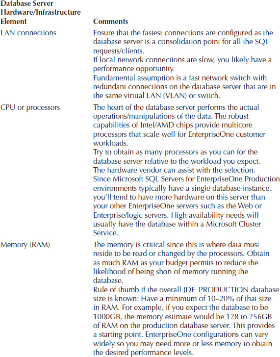

TABLE 9-3. Hardware Elements of Database Server
CPU or Processors
The SQL Server database depends on the processor being available to perform its work. As we stated, working with your hardware vendor on the machine sizing if you have good information of the workload characteristics will help greatly. With today’s Intel/AMD processors, you get a lot of “bang for the buck” in the commodity hardware. Typically we see higher-end blade or larger servers for the SQL Server database. Production environment databases are generally not virtualized except in some customer configurations where the user counts are relatively small, such as under 200 users.
NOTE
We are not stating that you cannot virtualize a production database, but make sure that additional planning, testing, and review occurs since you will be adding another layer of potential complexity that could impact your performance levels. |
When reviewing the processors from a tuning perspective, we examine the overall CPU usage of the machine from a high level using the various performance monitoring tools available in Windows and SQL Server. From a consulting perspective, if we start to observe average usage greater than 30- to 60-minute intervals above 70–80 percent, we need to investigate what is using the CPU time.
Most EnterpriseOne SQL Server databases tend to have sufficient processor capacity since more robust hardware is usually purchased for the database server. In one case, a customer was running SQL Server and observed very high processor usage especially during the month-end processes with heavy batch usage. They were using SQL Server 2000 SP3 Enterprise Edition, which had far fewer performance monitoring tools than we have today in Windows 2008 R2 and SQL Server 2008 R2. Using manual SQL scripts and Performance Monitor, we found thousands of queries that were performing full table scans (FTSs) and using full parallelism. Due to the parallelism settings and the high number of FTSs, they were consuming all the processor capacity for days at a time along with the buffer pool memory. They had gone through a couple of hardware upgrades over the years, increasing the processors and memory without purging the data to reduce the query response time or tune the FTS queries significantly. The system had in fact grown to a non-uniform memory access (NUMA) configuration with two physical servers merged to appear as one logical server. They were near a go-live to a newer EnterpriseOne release along with a database migration as well. The bulk of the effort went into the new EnterpriseOne release, and the needed indexes on several custom tables were identified and implemented. Query parallelism was also reduced along with eliminating the need for the more expensive NUMA hardware configuration. That tuning effort resulted in the processor usage being reduced significantly, and the month-end processes were reduced by more than 36 hours.
That example leads us into some database settings that can affect the processor usage for EnterpriseOne configurations. By default, SQL Server has the maximum degree of parallelism (MDOP) set to 0, which denotes that all available processors should be used. This setting is useful when your goal is to use all available resources to provide the fastest query response time. In an EnterpriseOne configuration, however, we want to reward the interactive transactions, and large queries that need to perform full table scans should not consume whatever resources are available. If you have a number of users and batch Universal Batch Engines (UBEs) along with external systems that may require performing an FTS on large tables with millions of rows, you may want to reduce the processor and resource consumption. The large throttle is the MDOP setting; by limiting the number of processors that a parallel query will consume, you will increase the execution time of the large query but reduce the processor usage so they are more likely available for the smaller OLTP queries in the system. Due to the large potential variations in EnterpriseOne workload characteristics, there is no hard-and-fast rule regarding the MDOP setting. For most customers, we recommend setting the MDOP either to 50 percent of your processors or, for large configurations with hundreds/thousands of users, to one or two processors. This reduces the potential for a small number of queries against millions of rows monopolizing your processors. Why reward the large user parallel queries with improved response time rather than the queries that are smaller and more efficient? For certain administration/operation tasks, you can normally set the MDOP higher if you need the resources.
For most EnterpriseOne configurations, we like to set the MDOP to 2 or 4 so that some parallelism is used by default to help the larger queries, but we still leave processor capacity available for other tasks. You need to develop a baseline of your configuration and determine the setting that works best for your business goals. There is no one best answer for all situations, but if you find that certain large queries affect the interactive transactions, this can be a very good option to consider. Table 9-4 provides a summary of our recommendations.
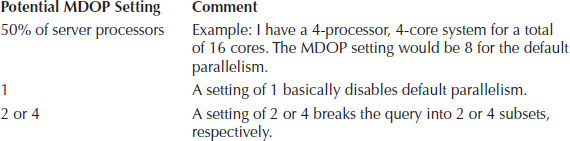
TABLE 9-4. Maximum Degree of Parallelism Setting
Generally, if you see high processor usage, you need to determine whether the issue is with SQL Server or perhaps other applications running on the server. For JD Edwards EnterpriseOne, we recommend that the database server be used only for the production instance and that other applications run on separate servers. Again, architecturally, you can combine multiple applications such as the enterprise services and database together, but you may not have the optimal configuration, especially if hundreds of users access the database.
Resource Governor
SQL Server 2008 also has a newer feature called the Resource Governor that can allow you to manage your resources between the online/OLTP users and various batch requests. Unfortunately, we have not observed or engaged any JD Edwards EnterpriseOne customers that are using this advanced feature. The Resource Governor could prove useful for larger configurations that want to reduce the priority and resource usage of larger or runaway queries. The Resource Governor can specify resource pools by a connection, which means that if you have a separate UBE or reporting server, it could be distinguished from the interactive workloads from the web and logic servers. This can then provide an avenue to prioritize your workloads between interactive and batch, if desired.
Areas That May Cause High Processor Usage
Following are some areas you should review that may be causing high processor usage:
Memory
SQL Server performs the database operations in the memory and reads/writes the changes to the disk system. One of the larger consumers of the memory is the buffer pool, where the data rows are referenced. The usage of the buffer pool can vary widely due to the large variety of queries JD Edwards EnterpriseOne business processes utilize. One of the main goals in the buffer pool use is to minimize the disk I/O and find the data in the cache/buffer pool. You cannot avoid all disk I/O, of course, but memory speeds are easily an order of magnitude faster or greater than going out to the disk subsystems. In a number of situations, the best disk I/O is the one that we don’t have to perform.
There are many different opinions on how much memory is sufficient for the SQL Server database. In our experience, it seems that whatever amount of memory is available, the database will use it. (Unless the total database size can fit into the memory of the server, which is rare for most customers.) We provided a general sizing rule of thumb of 10 to 20 percent of the total database size as a decent starting point for the server memory. There is no hard-and-fast rule that states you must adhere to this suggestion, but it at least provides a beginning for performance and scaling tests. If you tend to have mainly large batch queries that must scan through millions of rows, you will usually require more memory to hold those tables in the buffer pool, versus a customer that is highly tuned with mainly OLTP transactions that are very small in nature. Most JD Edwards EnterpriseOne customers fall somewhere in between, which is why the testing is so important to determine how the business processes operate in your configuration. If you don’t exercise the architecture with representative workloads you will most likely have several undesired surprises when you operate in production.
SQL Server dynamically manages the various memory areas it controls, unless you expressly override an area such as the Index Creation Memory or Minimum Memory Per Query database settings. For JD Edwards EnterpriseOne, the main memory setting that tends to be changed is the database Minimum Server Memory (in MB) and Maximum Server Memory (in MB). The default settings dynamically allocate/deallocate memory as needed and in cooperation with the Windows OS. This works well for test and workstation databases, but for a production level server, we recommend that the majority of resources be reserved for the database.
For production SQL Server databases, we suggest examining the Min/Max server memory settings along with the Lock Pages in Memory (LPIM) user on the SQL Server startup account. This is suggested for the latest Windows 2008 64-bit server configurations as well, even though this may be considered a bit controversial. (Some think that the latest SQL Server 2008 and Windows 2008 R2 no longer have this issue. Our experience is the occurrence is less frequent, but it still can occur.)
We suggest this configuration because we’ve noticed “unexpected” response swings that could not initially be explained after a system had been reviewed and tuned with application/index changes, and so on. Using Performance Monitor, we could see that during the slowdowns, the operating system was heavily paging and that the Memory/Available Mbytes counter was very low. In some customer configurations, we would see a warning in the Microsoft SQL Server error log about the working set being trimmed, and in other situations, no message was present. Some customers did have the Maximum server memory set to provide resources to the operating system, but did not have the pages locked. What we observed was significant paging when other applications were in contention with the SQL Server and the OS would page out large portions of the buffer pool. In a couple of situations, we did not observe memory pressure, and still the SQL Server working set was being trimmed back. Some examples that caused the issue were disk backups running from the operating system and large file copies of log files. So, as a general default rule, for production SQL Server, we tend to recommend LPIM.
Let’s walk through an example configuration to setting the memory:
Generally, the SQL Server should utilize no more than 80 percent of the server memory to leave room for other processes such as the OS, backup software, monitoring, and so on. If you have monitored the server for several months and find that you do not use all the OS memory and the database could use more resources, consider adjusting the memory. We are providing starting points that tend to work well in the majority of JD Edwards EnterpriseOne configurations, but every customer configuration has differences/requirements that can influence these configurations.
The SQL Server service startup account of sqlserver has been granted the “lock pages in memory” user right. When you start the database instance, you should see in the SQL Server error log a startup message indicating it has locked the pages for the buffer pool near the CPU detection message.
TIP
Review the Microsoft SQL Server Knowledge Base articles about how to enable the locked pages in memory setting. The SQL Server Enterprise and Datacenter editions for x64 simply need the LPIM user right assigned and the database started. However, the SQL Server Standard edition that JD Edwards EnterpriseOne supports has additional tasks needed for the x64 version, such as the potential application of SQL hotfix KBA 970070 and enabling trace flag 845 for versions 2005/2008 and 2008 R2. It is our understanding that in SQL Server 2012, the x64 editions will change and the LPIM user right will be all that is needed. |
If you decide that the LPIM is not an option for you, and you have multiple production database instances on the same machine, consider at least setting the min/max server memory settings to allow for dynamic allocation/deallocation of resources. If you do this, however, you may need to watch the Performance Monitor counters a little more closely and ensure that the paging levels are kept low for optimum response times. You can also use the LPIM for multiple database instances on the same server as well for each service account, but ensure that when you are locking the pages, each database instance’s maximum memory settings are all added up and the total of those instances does not exceed 80 percent of the physical memory. (You may even want to use 75 percent for the database instance total instead, since you will have more overhead running multiple database instances for the Windows OS to manage.)
Disk Subsystem
Your disk system is a critical element of the SQL Server database configuration. Typically the I/O subsystem is the slowest component relative to the processor and memory speeds. The network does not usually factor as much into the disk performance unless network attached storage (NAS) is in use. Most of the JD Edwards EnterpriseOne customer configurations we have observed tend to have dedicated disk and/or some type of storage area network (SAN) with multiple I/O channels present. The disk system tends to have high availability and reliability features such as RAID to minimize outages due to a disk failure.
It is very important that you understand the physical versus logical configuration of your disk subsystem. For example, if you have a SAN-attached set of drives that are presented as one logical F: drive, you need to know what the disk response time characteristics will be. If the logical drive has only three physical drives allocated, this may not provide the ideal response times if all your transaction data is running there. Likewise, if the SAN administrator has a large logical pool with dozens to hundreds of disks, he or she may state that it will perform very well without needing to worry about the physical disks present. In some situations this may be true, but experience has shown that you need to monitor the actual logical disk response times (which consists of queue + service times) to ensure that your database receives the desired access times. If the SAN disks are being shared with other applications/servers, you can sometimes have competing workloads or issues that affect your SQL Server database. We are not recommending that a SAN be totally dedicated for JD Edwards EnterpriseOne, even though some customers do that for the production architecture, but it is very important that you understand and monitor the servers on the SAN to ensure that they do not have a negative impact. The main thing is to communicate the disk response characteristics you want to use the database for in each of the major files. You may have to compromise for various reasons, but at least the potential impact to the JD Edwards EnterpriseOne database is documented.
Some SAN Examples
Following are a couple examples in which the logical presentation masks the physical complexity and interactions of the disk system.
First, in a client configuration, the SAN had the production JD Edwards EnterpriseOne database, enterprise servers, and a large data warehouse application. Overall, the JD Edwards EnterpriseOne system had very good response until the data warehouse extracts and reporting runs were initiated during the day. The overall disk response of reads/writes went above 400–500 ms and in a couple of situations caused the SAN controllers to reset due to the huge I/O requests from the data warehouse. The resolution was to separate the data warehouse to another SAN since they had reached the capacity of the present SAN. Once the workloads were separated, the contention was eliminated and the problem was resolved. The data warehouse requirements had pushed the SAN beyond its design limits, which impacted the response times.
Another example was a very large customer with hundreds of servers accessing multiple SAN devices with a fiber-based switch fabric. The production JD Edwards EnterpriseOne database had the logical disks separated, as recommended, between data, transaction log, and the TEMPDB. During the peak hours, the transaction log disk response would climb from 4–5 ms to more than 600–800 ms, which slowed down the entire database. No contention at the SAN disk level could be found, except for the slow disk response on certain servers accessing a particular set of SANs. Further investigation revealed that the SAN switch fabric had one Windows server that was not related to the EnterpriseOne architecture; this caused a “broadcast storm” of packets on the switch and affected a number of the servers accessing a particular SAN group. Once the fiber card on that Windows server was replaced, the intermittent issue was resolved.
For JD Edwards EnterpriseOne SQL Server disk and file layout considerations, we generally recommend the following for a production database, as noted in Table 9-5. Each of the major files has different disk response and I/O considerations. If possible, you want to separate these files to different logical drives for multiple reasons such as the following:

TABLE 9-5. Database Disk/File Considerations
TIP
If at all possible, at a minimum, separate your transaction log from the data/TEMPDB files. You want the transaction logs to be using the fastest performing drives as possible to ensure the best response times for the commits. |
From the operational aspect, it is suggested that you attempt to minimize the auto growth of these files in production. You can have the auto growth feature available, but if possible let it be the exception instead of the rule for the files to grow. Planning and maintaining the growth during off-peak hours can reduce potential response pauses that may occur if your database file has to be extended. Later in this chapter, we discuss the recommendation to preallocate the TEMPDB files on a production JD Edwards EnterpriseOne database to minimize waits for extent allocations.
We discussed that the disk response (queue + service) time is the important area to monitor and review for your production database. Generally for JD Edwards EnterpriseOne, you need a balance between OLTP and batch workloads for the disk system. OLTP wants very fast response times, while batch such as UBEs favor throughput to get as much data as possible. There are multiple methods to monitor the disk response time from your SQL Server database. Windows performance counters provide a wealth of information about your OS and various applications such as the SQL Server database. For JD Edwards EnterpriseOne, the main counters we tend to review are the Physical/Logical Disk for the individual drives of the OS and database.
Within the Performance Monitor (perfmon.exe), you would add counters for the following items. These are by no means the only counters you can use, but these provide good indicators of the disk response times to the database files.
These counters operate in the millisecond (ms) scale. Example: 0.005 = 5 (ms)
You want to see the SQL Server disk response at or below a certain level to ensure that the database receives the data in a timely manner. If the response times are high, you can almost be certain that the users or your batch jobs will be affected with slower runtimes. One caveat to note is that heavy batch workloads will tend to increase your disk response times since you are typically processing much more data, where we tend to have higher throughput (MB/s) than response time I/Os per second. So depending on your business process goals, you may need to strike a balance between the interactive users’ response and batch throughput. (This is one reason that heavy batch is executed during off-peak hours when possible to minimize disk response time concerns for the interactive users—that is, unless you have infrastructure that can allow concurrent interactive/batch processing.)
Understanding How the Logical Drives Map to the Physical
To determine which disk counter to use, you’ll find it helpful to understand how the logical drives map to a physical disk. You may have a one-to-one mapping of logical to physical, or you could have several logical drives using the same physical partition/device. For example, a C: and D: logical drive could be on the same physical disk in a RAID-1 configuration. The physical disk would provide Avg Disk Sec/Read info for the entire disk, while the logical would show you the response for that particular drive. Most of the time, we use the LogicalDisk counters to determine the overall drives response and then focus on the physical drives to understand how they map to the logical. You have to know the underlying physical disk presentation because contention could be causing response issues. A quick example would be where you separate your data, TEMPDB, and transaction logs to different logical drive letters, but you put all these files on one large physical RAID-1 disk configuration. Any of the three sets of files could cause contention issues with certain usage levels. The Windows Resource Monitor could tell you specifically which files have the greatest read and/or write usage on the disk at a particular point in time.
The disk response range that we like to observe is specified in Table 9-6.

TABLE 9-6. Disk Latency/Response Recommendations
Note that the averages should be sampled for durations of at least 15 minutes or longer if possible. If you start/stop the monitor for a brief period of time, such as 1 to 5 minutes, you may be observing a very narrow sample or window of time that does not represent the overall response time. The sampling interval is usually somewhere between 15 seconds to 5 minutes, depending on how long the duration of monitoring is desired. So if you were going to monitor for, say, 8 to 24 hours, the sampling interval should be 5 minutes to reduce the data you have to analyze. If the monitoring duration was 1 hour, you could set the sampling interval to 15–60 seconds.
Network
The SQL Server network component for JD Edwards EnterpriseOne typically does not require much, if any, tuning. The capacity of 1-Gbs or 10-Gbs Ethernet on switched networks with additional bonding/aggregation options tends to minimize tuning opportunities. The general recommendation is to implement the best networking infrastructure you can put in place. We know that is a generalization, but most correctly implemented network configurations tend to be the areas with least concerns from a tuning perspective.
Here is an example in which tuning/configuration was needed. One customer was running SQL Server 2008 R2 and Windows Server 2008 R2, and we noticed some messages in the JDE and SQL error logs regarding timeouts. The queries, when reviewed, should have been subsecond, and they intermittently timed out and had very long durations. We reviewed for cumulative patches and found those current. Examining the Windows 2008 configuration, we issued the command shown in Listing 9-1 from an administrative command prompt.
Listing 9-1 Check TCP interface settings
We searched for Chimney Offload state and found it enabled. In Windows 2003 Server this is enabled, and for Windows 2008 Server it is usually disabled by default. I suggested that we disable this setting on the database server since certain hardware vendor’s network cards have not always implemented this feature in an optimal manner. Using the administrative command prompt shown in Listing 9-2, we issued a command that is dynamic.
Listing 9-2 Globally disable TCP chimney
The TCP chimney setting that offloads to the network hardware had high connection counts, which a SQL Server can have in some cases. We have run into this situation with a few customers using certain network hardware cards, and if we observe SQL timeout messages occurring or unexpected batch response times, we review this setting. For these customers, when we disabled the TCP chimney, we observed a 25 percent reduction in the batch runtimes for longer executing jobs. For the interactive users, the important item was no evidence of timeout errors in the logs and hence they observed more consistent response times.
For Windows and SQL Server, we normally do not have to change any of the network settings or buffer sizes. With other JD Edwards EnterpriseOne platforms such as Unix/Linux and IBM System I, you may want to investigate further, because send/receive buffer sizes along with potentially jumbo packets may be viable options to consider.
SQL Server Configuration Ideas
Earlier we examined some major operating system areas that SQL Server utilizes. Remember that most tuning principles apply to whatever database platform you are using, so examine Chapter 8 as well for more information. In the following sections, we will discuss specific areas of SQL Server that we have found to benefit the JD Edwards EnterpriseOne configurations. We don’t cover every potential area, but we provide guidance for items that should give you the benefits that can influence JD Edwards EnterpriseOne implementations most frequently. Overall, SQL Server will perform very well if you have adequate hardware resources for the various workloads you may introduce. Tuning is almost always an option, but it may not be on the database side where changes need to occur. In effect, the main goal of a database server is to respond to the SQL requests presented with the lowest plan cost it can determine. Whether those requests are efficient or consume large portions of the configuration influences how well it can respond to those requests.
Database Configuration
Earlier we discussed the critical components of the SQL Server database configuration. Your main goal is to ensure that robust hardware components are in place to support the business processes and objectives for JD Edwards EnterpriseOne. You don’t always know up front what those business processes will be, but at some point in the project the processes will be in place so that a performance/scaling exercise can occur to ensure the operational goals can be met. Failure to confirm that the infrastructure will meet your business and software requirements increases the risk for unexpected issues to occur when the production workloads are introduced.
Assuming that you have sized the database server and laid out the memory, disk, and network with some of the previous recommendations, you can consider some of the following areas as well.
SQL TEMPDB
The SQL TEMPDB should be allocated with multiple files that match the processors available, as recommended for EnterpriseOne configurations. The default TEMPDB will allocate disk space dynamically, which means it extends and grows during the database operations. For larger database configurations, it is recommended that TEMPDB be preallocated evenly with a percentage such as 10 percent for expansion. This ensures that the temp database I/O will be more evenly spread and that processor latch contention will be minimized. The Oracle Metalink document ID 1275500.1, “Tips for Running EnterpriseOne with SQL Server 2008 and SQL Server 2008 R2,” has several good suggestions along with the appendix referencing a sample script to preallocate the TEMPDB files. It is strongly suggested that you consider this for production-level databases when using Read Committed Snapshot Isolation (RCSI), which we will discuss later in this chapter. The preallocated TEMPDB will improve overall efficiency and will assist the RCSI performance if implemented, since it utilizes TEMPDB heavily for the version store images. Even if RCSI is not used, we recommend using preallocated TEMPDB configurations.
Client and JDBC Drivers
A commonsense, but often missed, item is to ensure that all your client ODBC/Microsoft SQL Server Native Client (SNAC) and JDBC drivers are at the same levels as your patched database. This is one of those areas where different client drivers can affect the stability and performance of your system. It is one of the very first areas we check when reviewing a configuration for tuning opportunities. As mentioned, this is one of those “trust, but verify” items that should be reviewed for each server that accesses the SQL Server.
Database Statistics
The database statistics are another configuration area that is very useful to have enabled. At the database level, you would usually want the “auto create statistics” and “auto update statistics” options in place. Without good statistics in place, you may encounter a number of intermittent and inconsistent performance issues, since the database cost-based optimizer uses these statistics to determine the best access plan to the data. It is strongly recommended that for optimal performance you consider manual full-scan statistic updates on at least a monthly or quarterly basis. A number of customer configurations achieved noticeable response improvements just by ensuring that the statistics were up to date. Consider the options in Table 9-7.

TABLE 9-7. Statistic Options to Consider
TIP
When you’re considering running manual statistics, be sure to cover all your production databases, which include the JDE_PRODUCTION, JDE910 (system, object librarian, data dictionary), and JDE_PD910 (central objects, versions, serialized objects). With package builds and deployments, we have seen a number of configurations in which the central objects Java serialized objects tables F989998/F989999 did not have statistics present. The web response for that instance would load the applications slower initially as a symptom. With the later JD Edwards EnterpriseOne releases using XML specifications, the database is critical as well for both the web and Enterprise server to retrieve those specification records in a timely manner. |
Database Recovery Level
Ensure that for production-level databases you enable the full recovery model instead of the simple recovery model. You want to back up the transaction logs so you can have a point-in-time recovery of the transactions. Most customers’ test environments use the simple recovery model, but if you do that for production, you can only recover the database to the last backup point, which may be days or even a week old. There is increased operational maintenance in ensuring that the transaction logs are backed up, but if you do have some type of disk failure or data recovery for required tables, you have many more options if you can restore up to a certain point in time. A very small number of JD Edwards EnterpriseOne customers use the simple recovery model for production databases, and we have always made sure that their management understands and signs off on the recovery limitations present.
Other SQL Server Features
SQL Server also has a large number of features that we will not discuss in this chapter since the complexity and design are complete engagements that can takes weeks to months to fully design, architect, test, and implement. We discuss architectures and high availability in other chapters, but specific vendor implementations can vary widely.
Several viable options are available to increase availability and performance for various business requirements. Options such as log shipping and replication allow you to create a copy of the databases for disaster recovery, backups, and read only reporting/query activities. Database mirroring can increase high availability options. SQL Server 2012 using the AlwaysOn availability groups increases the flexibility you have while consolidating several of the features mentioned for easier administration of DR, backup, and reporting environments.
We suggested that if your business requires a large number of ad hoc–type SQL queries from users or reporting tools, you may benefit by moving those users to a replicated or mirrored database instance instead of running those queries on your production JD Edwards EnterpriseOne database. Each customer situation is different, since the architecture can have many influencing factors along with the business processes in use, and this means there is no one-size-fits-all recommendation.
Note that once JD Edwards EnterpriseOne certifies Windows Server 2012 and SQL Server 2012, additional options may be available at the OS and database levels that we cannot currently discuss in this book. You can, however, leverage a number of configuration areas in SQL Server 2005 and 2008/2008 R2 that are built upon in the 2012 editions, so it helps to watch those technologies as well. Basically, the majority of recommendations in this book should apply to the SQL Server 2012 release as well.
Production Parameter Settings
The following are some SQL Server parameter settings at the instance or database level that you should review. We discussed some of these settings earlier in this chapter, such as the min/max memory and MDOP, so they will be reinforced here.
EnterpriseOne Databases May Initially Be Set to 80 SQL 2000 Compatibility
It is generally recommended that once JD Edwards EnterpriseOne is installed, each database be changed to level 100 for SQL Server 2008/2008 R2 to enable that database functionality. (This assumes of course that you are running SQL Server 2008/2008 R2; adjust the setting to your appropriate database version.) See Table 9-8.
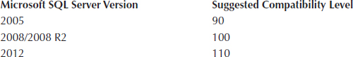
TABLE 9-8. Suggested Compatibility Level for Each Database Version
If you are running later releases of JD Edwards EnterpriseOne, you’ll probably be using SQL Server 2008 or 2008 R2. If you leave the setting at the 80 level, you may restrict certain database capabilities/features available. This can sometimes create unexpected behaviors in the database, since you are limiting the functionality to an older release. You can find the settings at older levels when you first install, upgrade a database server, or restore a database. Compatibility level is mainly intended as a migration aid and not as a long-term solution, so you want JD Edwards EnterpriseOne to leverage the functionality available in the SQL Server database release you are using. Make sure you change this setting only when there are no active users attached to the database, or you can risk impacting active queries.
Server Memory Options at Instance Level
We discussed the minimum and maximum server memory options and the use of LPIM. The main goal here is to set a maximum server memory (in MB) that does not overcommit your memory resources. For test databases and virtual machines, you may consider using dynamic memory management without the LPIM, but for production databases on physical hardware, we recommend using LPIM and ensuring that you leave enough memory for the OS and other processes on the database server. The minimum server memory (in MB) is useful for test databases and virtual machines to ensure a certain amount of memory is reserved for the SQL Server database instance when dynamic memory management is in use. For production database instances using the LPIM setting, the minimum and maximum memory settings are the same to preallocate/reserve the memory. Virtual machines (VMs) have additional special considerations, where the minimum memory setting influences the amount you reserve for the guest VM to minimize the risk of ballooning the guests and causing large amounts of paging, which impacts response time in most situations.
Maximum Degree of Parallelism (MDOP)
The SQL Server database instance Advanced setting can be changed from 0 to 1 or 2 for multiple processor configurations if desired. More details were provided earlier in the chapter for potential settings you can consider. This can reduce database locks by limiting parallel queries to one or two processors instead of all of them. No or low parallelism effectively prevents a large SQL query from “taking over” several processors and affecting other SQL queries. The large SQL query can take slightly longer to complete, but it will not slow down other queries in the system. This setting requires a restart of the database server to take effect. Some customers like to utilize all the processors for large queries, while in busier customer configurations we have found that limiting the parallelism provides a more consistent response for the interactive users, without penalizing the large queries completely.
Performance Monitoring and Index Review
Microsoft provides a number of very good performance collection tools that can be used at the OS and database levels. Prior to SQL Server 2005, you would tend to use SQL profiler, scripts, and the Performance Monitor to obtain insights into the database and Windows OS. Third-party monitoring tools are also available that ease some of the data collection and evaluation tasks if you elect to utilize those products. Windows 2008 and SQL Server 2008 offer many additional features to collect and monitor the performance of the database server.
Some of the performance collection tools available in Windows 2008 Server and SQL Server 2008 are listed in Table 9-9.

TABLE 9-9. Microsoft and Other Monitoring/Performance Tools
These provide starting points that can benefit your staff and any consultants assisting with tuning/performance efforts. Using these tools helps identify potential opportunities or issues within your architecture, and each offers a number of features when you focus on a certain area of the database server. The various real-time monitors provide feedback as events occur in your system, while other tools can capture and store for historical purposes how your system is operating. The third-party tools such as Dell/Quest Spotlight for SQL Server, and Idera SQL diagnostic manager have dashboards and performance recommendation capabilities that can assist you in determining database events and potential corrective actions. Your comfort level, training, expertise, and time availability can influence the value the performance monitor tools can bring to your configuration. We have observed a wide spectrum of customers use a number of tools, and they have various degrees of knowledge, training, and experience to utilize them. Some implement the performance tools more completely than others.
The main point with any performance monitoring is if you don’t track and baseline the events, it is difficult to measure/quantify any changes you make to the system. As stated in Chapter 8, you can make relatively simple changes that can have limited or very broad impacts to your configuration. Knowing where your system has been and how changes affect it are extremely important.
Index Review
Once you have good performance monitoring baseline information in place to see how your system is performing, you can utilize performance tuning diagnostic checklists to identify potential areas to review. We always like to start at the application levels and work through the operating system and database. Remember that the database simply responds to the SQL requests presented to it. The more efficiently designed the application and user SQL queries are, the better the database typically is able to return the results in a timely manner. Assuming that most of the Windows OS and SQL Server configuration items are in place to provide adequate resources based on the workload presented, you invariably tend to get drawn down to creating indexes.
When examining a customer configuration, we typically go through the performance tuning diagnostics and ensure that the overall architecture and related components are working well together. Index review tends to be near the end of the list of items reviewed, since you want to ensure a firm foundation is in place before changing the database. There are many good reasons to add an index, but it is a balancing act to ensure that large numbers of indexes are not added that could possibly cause negative performance issues for the tables under review. Remember that each added index can increase the overhead to be maintained, stored, and scanned along with the other indexes on that table. If the table has millions of rows present, the maintenance to perform modifications can become significant.
JD Edwards EnterpriseOne delivers a number of indexes that are fairly comprehensive for the base applications delivered. This does not mean that every column for each table is indexed, which would be impractical, but for the majority of business processes, you will typically have a usable index for that table. However, there are a number of situations in which a business process or application is designed to use columns that may not have an efficient index available for that particular procedure. These can become opportunities for which it makes sense to consider an index. Some example situations are listed in Table 9-10, but these are by no means all the situations that may require an index. Typically, the situations most noticeable are for queries against large tables, but that is not always the case, since you could have thousands or millions of smaller SELECTs that take a few tenths of a second, and that would add up significantly.
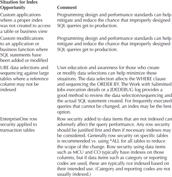
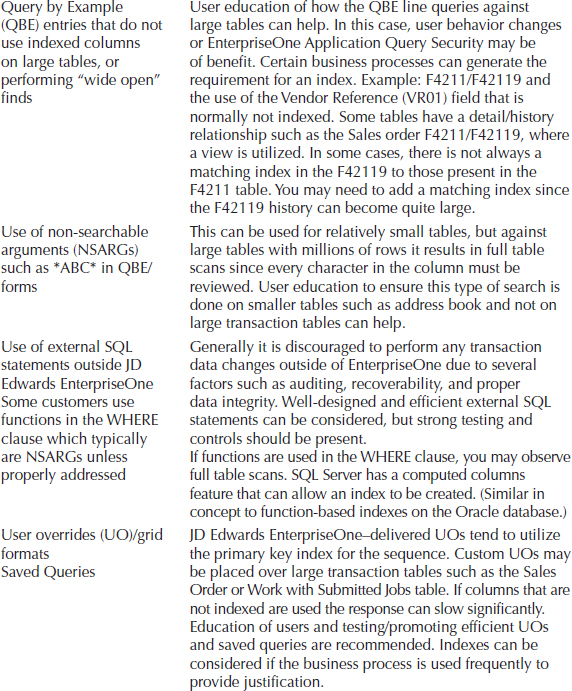
TABLE 9-10. Potential Areas That May Require Additional Indexes
In a number of situations, an index can be justified, as you can see from the examples in Table 9-10. When we are to the point in the performance checklist where you review index opportunities, we like to consider the following process to justify the creation of an index. Following the gears and cogs principle, we want to address the largest influencing areas first and then, if needed, focus on the smaller opportunities that have less impact.
In some customer engagements, we’d see the SQL Server administrator use the tuning index wizard/advisor and then attempt to create all the indexes that it recommended. In our opinion, this is a very general and blanket approach that does not tend to be very successful. It is better to establish the baseline of how the system is operating, and identify the potential opportunities and how to address them, whether they are application and/or database tasks. If the change(s) do come down to index opportunities, we tend to take a very measured approach to introduce them in small groups at a time depending on the customer circumstances. If you start adding dozens or hundreds of indexes, how can you monitor/measure and evaluate all those changes effectively? We use the multiple pass method and address the indexes that can have the greatest impact, monitor them, perform another cycle of the monitoring, and measure and tune to evaluate the effect. Once those indexes are in place, we usually have new opportunities trickle to the top of the list and we continue the process over days, weeks, or months until we reach the business goals desired.
So how do you determine which index opportunities are the ones to address first? You can consider a number of factors to prioritize which index changes can have the most immediate impact. Table 9-11 lists some of the criteria that we have used during customer engagements to help prioritize which index changes can have the most immediate effect.
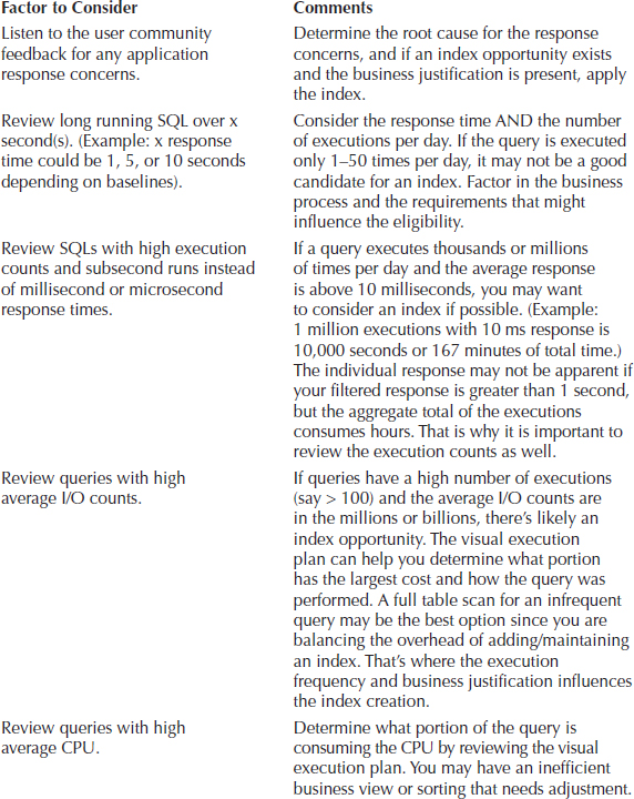
TABLE 9-11. Potential Index Criteria Factors to Consider
So to review index opportunities, we want to reduce the query response time, and this can be considered for queries that consume a high amount of I/O or CPU. The execution count is the main factor that can influence whether an index is justified, since if you execute a query only a few times per day versus a query that is executed hundreds or thousands of times, you will usually obtain more benefit reducing the resources consumed by the higher execution count. If there is a critical business process, such as the timing for a financial closing processes, it may justify the index. One of the key points is to utilize a measured and managed approach to indexes and not blindly introduce them to see what may work. The goal is to balance the resources available in the SQL Server as well as you can to provide consistent response to the application queries.
Dynamic Management View Reports
In the previous sections, we mentioned DMVs and that SQL Server 2005 introduced these views. From the SQL Server Management Studio you can access a large number of standard DMV reports at the database and instance level. You can also access the DMVs yourself if desired via SQL, but for JD Edwards EnterpriseOne tuning purposes, you can obtain most of the critical information using the standard reports delivered with the database. If you like to delve into the details, you’ll find a large number of Microsoft documents and blogs available that provide examples of SQL queries using DMVs.
So what is the greatest benefit of using the DMV reports from the JD Edwards EnterpriseOne perspective? Well, in past consulting engagements using SQL Server 2000 and early 2005, we would need to rely on a combination of several performance methods to identify database and index opportunities. SQL Profiler, Performance Monitor, custom SQL scripts, JD Edwards EnterpriseOne debug logs/Performance Workbench, or third-party tools would be needed to identify suboptimal SQL or resource bottlenecks. Now the standard reports using the DMVs in SQL Server 2005/2008 and beyond consolidate and provide this information. The other tools still have their benefits and place, but it is now easier to obtain the desired events you are attempting to measure/monitor.
The DMVs are not the complete solution to every tuning exercise, but they do provide some very good insights to identify what is occurring within the database that can lead you to other areas. We wanted to list some of the standard reports you may find useful when reviewing your JD Edwards EnterpriseOne database. Figures 9-1 and 9-2 show examples of accessing a standard Disk Usage by Table report from the SQL Server Management Studio application. This provides a quick list of the tables in that database along with details such as the number of records and space used for data/indexes. You can also print or export the report, which provides additional flexibility for review or scripting tasks. Another option is to take the DMV and create your own script to manipulate the data returned as desired, such as listing tables over a certain size or row count.

FIGURE 9-1. Launching a database Disk Usage by Table report
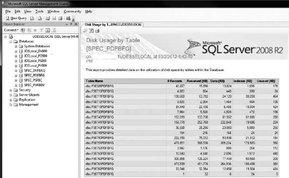
FIGURE 9-2. Disk Usage by Table
Table 9-12 shows some of the standard reports that we utilize when reviewing a JD Edwards EnterpriseOne database for tuning opportunities. You may find others that apply to your situation as well, but these provide some real-time queries. We also provide some comments regarding how the report may be utilized.


TABLE 9-12. Suggested DMV Standard Reports
More than 100 DMVs are available and can provide database information along with the ability to create custom reports if desired. As you can see, with the standard reports you can obtain a number of insights into your database without having to create SQL scripts. (You are welcome to create your own scripts as well, which many administrators do.) As field consultants, we have found most of the performance tools available provide very good information to monitor and measure how the database is performing.
Database and Backup Compression
With the introduction of SQL Server 2008 Enterprise and Datacenter editions, the ability to compress at the row or page level was introduced for several datatypes. In SQL Server 2008 R2, support for Unicode datatypes was also added, which covers the majority of data that JD Edwards EnterpriseOne utilizes.
One of the key elements of database compression is that you reduce the overall number of bytes stored on the disk and in the buffer pool if your data can be compressed. You essentially have more rows per 8K data page, which in turn reduces the number of disk I/Os needed to retrieve the data. As with most situations in life there is no free lunch, however, since there is additional processor overhead and time needed on the database to compress/decompress the data. However, if your database server is not CPU constrained (such as average CPU usage below 70 percent), you may be a good candidate to consider compressing the larger JD Edwards EnterpriseOne database tables. You have the option of using row- or page-based compression.
From our experience, we consider using the page compression for customer databases that are 1.5TB or smaller because it works very well with the type of data stored in JD Edwards EnterpriseOne. If your database size is greater than 1.5TB uncompressed, we typically consider using row compression due to the lower overhead involved. Row compression is used for very large tables, because page compression could take significantly longer for maintenance tasks such as index rebuilds. There is nothing to prevent you from considering row compression, but you tend to see better disk savings by using the page compression option. Also, you can use different compression options on a per-table basis, but most customers tend to gravitate toward either row or page without mixing them. The bottom line is that an analysis of your infrastructure and business needs should be conducted to determine which compression option may be best for your company.
You will need to ensure that your SQL Server 2008/2008 R2 edition is Enterprise or Datacenter, because this feature is not currently available in the Standard edition. To take full advantage of the compression option, you need to be running SQL Server 2008 R2 or later, where the Unicode compression is included as well. If you are using the earlier 2008 release, there are still advantages to compression, but it will depend on your JD Edwards EnterpriseOne installation data. If you are a new install, your database would be using Unicode data; if you upgraded from a previous release, you may still have your data in the non-Unicode format for business data/control tables. We have done database row or page compression for both configurations with very positive results. If you can leverage the maximum potential, however, it provides the most cost-effective benefit.
Several JD Edwards EnterpriseOne customers using SQL Server 2008/2008 R2 have implemented row or page compression. If you can use SQL Server 2008 R2 and a supported JD Edwards EnterpriseOne Tools level, the combination provides the maximum benefit currently available. One of the considerations for JD Edwards EnterpriseOne is that most of the data columns are populated with data, since null values are typically discouraged. This is a great benefit for database compression since a large number of columns, even if “empty,” will either have zeros or spaces in them. This helps increase the ability to compress the tables and indexes. We have observed very good compression improvements (3 to 12 times better) for some tables, depending on the data in those tables. Overall disk savings can be double-digit percentages, which allow more database pages to be stored in the buffer pool, and which in turn can reduce I/Os needed to retrieve the data.
Generally, the approach we utilize is to run the sp_estimate_data_compression_savings stored procedure against the business data and control tables schemas (for example, CRPDTA and CRPCTL) to get a general estimate. You should perform the actual row or page compression on the data and indexes only when you have exclusive access to that database, such as during a planned outage. You can take the results from the stored procedure and then use that list to sort by the tables over a certain size, such as 100MB, or a particular row count. Mainly, you want to compress tables with data present and leave smaller tables uncompressed to minimize the overhead. We have used both T-SQL scripts to generate the statements for the compression and taken a list and created a copy/paste of the table/index names into the SQL statements.
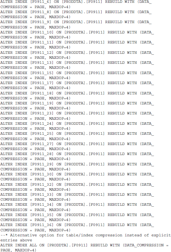
Regarding the compression, note that you should utilize the parallelism (MDOP) option as much as possible. Table compression can require several hours, depending on the amount of data you have. For example, one customer on a relatively small configuration with a 400GB database took about 3 hours to compress all the selected tables to about 37GB. It is strongly recommended you test the compression on a copy of the data in prototype to determine an approximate runtime for the production compression. Listing 9-3 shows an example of using page compression on the JD Edwards EnterpriseOne F0911 table with two different approaches.
Listing 9-3 Example page compression syntax for data/indexes

You can use the database backup compression option to compress the backup file even further when you utilize database row/page compression. With compressed data and index tables you should observe a measureable reduction in the backup and restore times for your database. (Makes sense: with less data backed up there is less to restore saving time.) Even if you do not choose to use database row/page compression you should strongly consider using compression on your database backups to save disk space. It does utilize more processor capacity, but if you have it available you reap more benefits than negative consequences. We have observed some customer’s database backups decrease from hours to minutes and the backup file size be 5–10 times smaller than the database when both database page and backup compression are in use. Just make sure you are not CPU-constrained before going down this path or it will cause additional resource and response issues.
There are many benefits to considering SQL Server database row/page and backup compression, and you should look into it if you have the edition that provides this feature. All of our JD Edwards EnterpriseOne customers that have implemented these compression strategies have seen significant reductions in the database disk storage, backup times, and incremental improvements in batch runtimes, since more data was available in the buffer pool.
Read Committed Snapshot Isolation (RCSI)
Since the early JD Edwards releases such as OneWorld Xe, there has been a little-known JDB database feature regarding SQL Server queries. The SQL Server database utilizes a pessimistic locking mechanism, where both read and write locks are present when a row is accessed. This is a very good database locking model for most situations, but for highly interactive applications such as JD Edwards EnterpriseOne, with both interactive and batch SQL requests against the same tables, you can observe increased locks and blocks. If you introduce ad hoc queries or reporting tools such as Microsoft Access ODBC, you increase the opportunity for locks to be held for long periods of time, which negatively affects web and batch applications.
JD Edwards introduced a query timeout and retry mechanism that would run a query for a few seconds and timeout/cancel that query if it exceeded the timer. It would retry several times and then modify the SQL query to use the
NOLOCK option, which can be observed in JDEDEBUG logs when that situation occurs. By using the NOLOCK option, the query would read uncommitted data and allow it to complete. You might have a UBE or large user query against thousands of rows holding read/update locks that would prevent interactive applications from accessing the record. With the query timeout on JD Edwards operating under the covers, you would see a delay in your interactive users’ query or UBE, but it would eventually process and not be blocked. We call these blockages caused by large numbers of user requests a “block party,” since everyone attempting to access that table or resource waits together until the blocker releases its lock(s). Overall, this mechanism worked well for JD Edwards OneWorld and EnterpriseOne, but it did cause some response time fluctuations during heavy contention that most customers could not explain.In SQL Server 2005 and later releases Read Committed Snapshot Isolation (RCSI) was introduced. This database setting uses row versioning to provide read-committed isolation levels and relies on creating an image of the committed records at the time of the
SELECT queries in TEMPDB. This effectively prevents SELECT statements from holding read locks and blocking other read requests to the same tables. The largest effect for JD Edwards EnterpriseOne is that overall throughput improves for interactive and batch users due to reduced blocking. Update/delete lock isolation levels are still present by SQL Server, so your data integrity is maintained. This is sometimes called optimistic locking, which has been used by other database vendors over the years.Here’s an example in which this effect is most noticeable: A user with a third-party tool using ODBC access can hold a large number of locks if they access the transaction tables. These locks can block UBEs or web users from retrieving or updating the data in some situations. EnterpriseOne has specific code built into its tools for SQL Server that allows it to timeout queries and then eventually switch to a read uncommitted or
NOLOCK option. This can help inquiry SQLs, but will not help a user that needs to delete or update certain rows. RCSI basically prevents reader threads from blocking writer threads in the database. This provides better response to the user when larger SQL queries are present. However, there is an observable increase in the TEMPDB database usage and size since the version store is present. The rows at the start of the SQL SELECT statement are saved in TEMPDB as a “version” to ensure a consistent read occurs. In later JD Edwards EnterpriseOne tools releases, we worked with development to enhance the query timeout settings so that we could utilize RCSI and correspondingly change our settings to disable the query retries and timeouts for SQL Server.The method to change this requires the database to be in single user mode, and changes to the Enterprise server and Web server query timeouts are recommended to minimize the chance the
NOLOCK option will be used. A Tools version of 8.97.2.x or higher is recommended to use these features properly. On the SQL Server databases such as JDE_PRODUCTION and JDE910, you can use the statements in Listings 9-4 and 9-5.Listing 9-4 Query to determine if RCSI is enabled
NOTE
Databases with RCSI enabled will have a value of 1 and others will be at 0 to indicated disabled or default pessimistic locking. |
Listing 9-5 Enable RCSI on database (ensure no active users in database)
Once you have the databases identified and changed to enable RCSI, you will also need to review the EnterpriseOne JAS.INI and Enterprise Server JDE.INI settings. In the JAS instance JDBJ.INI file under the [JDBj-RUNTIME PROPERTIES] stanza, you need to disable the JDBJ query timeout and retries. Note that you may have to add this manually if you can’t locate it through Server Manager for the Web instance.
Here is a description of what these two settings do along with the default values:
This indicates the maximum number of times a SQL Server query will be executed within the specified
msSQLQueryTimeout period (see msSQLQueryTimeout details); then the last attempt of query execution will append the SQL statement with the NOLOCK syntax. This last attempt should retrieve data, but the data may be uncommitted or “dirty.”The retry attempts are made only when following SQL error conditions are detected:
The JDBJ settings have a SQL Server query default of 10,000 ms, or 10 seconds, and will retry two times before switching to the
NOLOCK option on the third attempt. This means that if it performs three retries, each one takes 10 seconds, so the entire query could be 30 seconds or longer.On the Enterprise server JDE.INI file under the [DB System Settings] stanza, the SQL Server query default is 1 second with 17 retries before the
NOLOCK option is used. That means a minimum delay of 17 seconds can occur if a query goes to the NOLOCK option. This was used mainly for the call object threads to reduce the wait time, but if you have a table with heavy locks it can significantly slow down the runtime of the queries for that application. This also affects the batch UBE queries that run on the Enterprise server.The default settings apply to JD Edwards EnterpriseOne when running SQL Server and using the default record locking settings, which is pessimistic locking. If Read Committed Snapshot Isolation (RCSI) is enabled at the database level, you should disable the JD Edwards EnterpriseOne SQL Server timeout/retry settings using the parameters shown in Table 9-13.
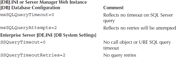
TABLE 9-13. JD Edwards SQL Server RCSI Query Timeout Settings
NOTE
These parameters became available in Server Manager starting in Tools 8.98.4.2 to review and have been present in earlier 8.97/8.98 Tools releases if you manually added them to the INI settings. |
Generally, if RCSI is utilized, you want to change from the default settings so that you do not utilize the
NOLOCK syntax or query retries since that can delay the SQL statement response or perform a dirty read. The query may actually take several seconds, just as it would with default locking, so you don’t want extra retries present with RCSI in use.Again this recommendation should be used only if the SQL Server database has implemented RCSI to eliminate contention between database readers and writers. If you simply want to adjust the timeouts and utilize the
NOLOCK option, you can certainly consider that option as well, but we have found from customer engagements that the RCSI option works very well. Every customer for which we have implemented this feature on a JD Edwards EnterpriseOne database has provided very positive feedback, and the result has been improved response with timeouts reduced significantly. Once the INI settings are in place with coordination of the databases enabled with RCSI, no customers to date have requested to return to the default locking model. In most situations, the blocking and transaction timeout effects are significantly reduced or eliminated.Tuning IBM System i Database
The IBM System i (formerly known as IBM iSeries or AS/400) is a very robust integrated platform that includes the DB2/400 database integrated with the OS/400 operating system. The JD Edwards EnterpriseOne application roots sprang forth from the JD Edwards World Software functionality and it is a very viable platform with a wealth of robust features and capabilities. The current V6R1 and V7R1 OS releases with associated cumulative patches applied provide an excellent configuration that can automatically manage a large number of jobs. We ask our customers, “When was the last time you met an IBM System i database administrator?” We are not stating that there are no tuning opportunities available to maximize the performance of the IBM System i by any means, but the integrated nature of the architecture allows it to self-manage for a number of customer configurations.
The two most critical areas that are similar to what we have stressed for other platforms are performing an accurate hardware sizing with your vendor and ensuring that the IBM System i OS cumulative patches are relatively current. We understand that keeping the cumulative patches current is viewed by some as a disadvantage that can potentially affect the applications. It has been our experience, however, that if solid application testing processes are in place for the critical business applications and time/resources are made available to stay current, your system tends to have fewer issues and provides flexibility to adopt new changes in the JD Edwards EnterpriseOne application.
You can find a large number of very good documents regarding tuning the IBM System i. Overall we believe that these provide a very good foundation to tune your configuration and that the other databases did not have quite as much JD Edwards EnterpriseOne materials written about them.
In this section, we highlight certain areas to consider without the extensive detail. Some of these tuning recommendations are also contained in “IBM Power Systems with IBM i Performance and Tuning Tips for Oracle’s JD Edwards EnterpriseOne 9.0” and certain elements from the IBM JD Edwards website referred to in the JD Edwards EnterpriseOne MTR documents (www-03.ibm.com/systems/i/advantages/oracle/). There are a number of IBM documents, Redbook and white papers available that provide additional tuning insights for the EnterpriseOne applications running on IBM System i. IBM has also published a good paper for smaller customer configurations since a number of these recommendations apply to most JD Edwards EnterpriseOne configurations. When you have a single processor with limited memory and disk you actually may need to tune a little bit more since fewer resources are available that need prioritization.
Following are some areas that affect the JD Edwards EnterpriseOne configuration performance. This is not a comprehensive discussion, but it provides some good areas for you to investigate and consider if you do not already have them in place. Ensuring that you have prestart allocations and shared memory pools properly configured can help significantly. Reviewing the large number of documents, guides, and papers, along with considering consulting assistance, can also be of great value. Experience and understanding your business processes can help in tuning the system. Properly sized hardware for your workload to obtain a balanced IBM System i database platform is the main goal.
Performance Collection
It is normally recommended that you enable the Collection Services and allow performance data to be available for review. System i Collection Services has a very low overhead for performance gathering and is strongly recommended. It allows you to review your system from a historical perspective for a certain window of time, such as seven days. Collection Services automatically purges the older data and tends to use a small amount of disk space. You can have this data sent to IBM support for assistance; or, if you want to perform a JD Edwards EnterpriseOne sizing, you can see where this data is utilized in the analysis.
In the IBM System i versions, such as V6R1 and V7R1, the System i Navigator is the preferred method for initially reviewing the performance data. More detailed performance tools, such as iDoctor and Performance Explorer (PEX), are also available. We are not going into detail regarding these tools; you should use the System i Navigator tool when possible for reviewing system performance. The historical and graphical information is easy to use and identifies potential bottlenecks such as high processor consumers or hot-disk issues.
Database Index Configuration
The System i has a very robust database (DB2/400) integrated into the OS. One of the advantages for JD Edwards EnterpriseOne configurations is that it will automatically create a temporary index for a query that can be reused by other applications. Some customers may notice that after an Initial Program Load (IPL), the system may appear a little slower in response, and over the course of a few days it will “speed up.” Some of this may be due to temporary indexes being created.
You can utilize the IBM System i Navigator to review the SQL Cache and indexes that are present. At that time, you can decide whether you want to create a permanent index via the Navigator or from the JD Edwards EnterpriseOne OMW toolset. There are a number of opinions regarding where custom indexes should be created and maintained. We think that you should leverage the resources you are most comfortable using to document and maintain the custom indexes. If you have a System i administrator who documents and maintains the indexes, that is a good thing; or if you have strong change management and development resources for JD Edwards EnterpriseOne, you can maintain them there, where the index will be more readily visible to developers.
Index opportunities utilize criteria similar to what we discussed earlier in the SQL Server sections of this chapter: you assess the need for the index based on business requirements, executions, and what response time is desired. The Navigator provides a very easy method to monitor the queries in use and filter/review by many criteria such as most expensive time, executions (total times run), average processing time, and so on. In Figure 9-3, you can see an example of some SQL statements from the SQL Plan Cache.

FIGURE 9-3. SQL Plan Cache index review
Navigator makes it very easy to review the SQL statements, provide a visual explain plan, and generate a custom index if desired. You can also determine the temporary indexes that have been created and how many times they have been executed. This can allow you to decide whether you want to create the index permanently.
TIP
If you elect to create indexes via a script outside of JD Edwards EnterpriseOne, we would strongly suggest that you save all the custom index creation SQL in either a single text file or a folder with the names of each index. This will allow you to track and document the custom indexes added, and if you update or upgrade in the future it will allow you to easily reapply them after reviewing their validity. Use a naming convention to identify the indexes easily. (Sometimes an index is no longer needed when you make business process changes or implement new modules, so it helps to review whether an index is being used.) |
JDE.INI and QAQQINI Settings
Every CNC administrator who installs or upgrades JD Edwards EnterpriseOne should review the installation/upgrade guide for JD Edwards EnterpriseOne. The latest JD Edwards EnterpriseOne 9.1 install/upgrade guide contains a large number of useful configuration settings that should be reviewed. We have found several customer configurations where simply implementing the recommendations in the JD Edwards EnterpriseOne installation/upgrade guide would save time and frustration. One small example is ensuring that the Enterprise server JDE.INI
SQL Package Library=2 setting is changed to a 0 or 1 after the install/upgrade. We have seen this set to 2 at many customer sites, which increases UBE runtimes and SQLPKG entries significantly.Every JD Edwards EnterpriseOne configuration on System i must create a
QUSRSYS/QAQQINI in order to increase the LOB_LOCATOR_THRESHOLD to 10,000, or your package builds will be challenged. In addition to this user setting, you can consider where you want the SQL Query Engine (SQE) to have different optimization goals such as *FIRSTIO or *ALLIO. For the majority of customers, the default of *ALLIO works very well between web requests and batch jobs. However, some customers have primarily web-based users with very little batch requirements. Others with more diverse requirements may want the best of both options by setting *FIRSTIO as the default optimization_goal option in QUSRSYS/QAQQINI and have a custom library for the QAQQINI setting such as UBEBATCH/QAQQINI with the *ALLIO optimization_goal, where the batch subsystem jobs have a routing entry use the CHGQRYA command to use the UBEBATCH/QAQQINI settings instead.Basically what the
QAQQINI optimization_goal does is influence the SQE (we are assuming that all your queries are utilizing SQE and not the older Classic Query Engine [CQE], which can use this parameter as well) to favor using indexes to return initial data as quickly as possible for *FIRSTIO. The *ALLIO default setting for most connections is designed to return all the data, which works well for most customers except those that want to provide the interactive web users some better query response times where the data appears before the query completes. So if you want, you can consider one of the above options for your configuration and see how it benefits your system.Use the IBM System i Navigator and review your ODBC/JDBC and batch job SQL plan cache in detail. The details of the query can tell which
optimization_goal and SQE/CQE engine is in use. In the V6R1 and V7R1 OS releases, you may find that the desired optimization_goals are already in use. ODBC/JDBC typically utilizes *FIRSTIO, and batch jobs may be using *ALLIO, depending on your configuration.TIP
One hardware change that can also improve I/O response rates is to investigate the option of using Solid State Drives (SSDs) for a portion of your IBM System i. IBM System i V7R1 and later releases utilize these drives with increased flexibility, and this typically improves your overall system response such as UBE runtimes. These drives may be beyond your budget, but if you can include them in your configuration with relatively current IBM System i hardware, you could be pleasantly surprised. You may also be able to obtain hardware sizing information from IBM to aid in the decision and potential benefit of using these drives. |
Job Prestart Allocations
A very useful change that impacts JD Edwards EnterpriseOne significantly is ensuring that you allocate sufficient QSQSRVR and
QZDASOINIT prestart jobs that are ready to accept database connections. Unfortunately, although the JD Edwards EnterpriseOne installation/upgrade guides recommend how to prestart the QUSRWRK/QZDASOINIT, for some reason the more heavily used QSYSWRK/QSQSRVR prestart settings are not documented. Some Oracle Metalink documents show how to do this, such as ID 841314.1 and the EnterpriseOne installation/upgrade guides. The method used for QZDASOINIT prestart jobs is the same for QSQSRVR jobs, so ensure that you have prestart levels configured for both. With the later releases of JD Edwards EnterpriseOne, the QSQSRVR jobs tend to be more heavily used for database operations than external connections via QZDASOINIT. External connections such as web servers, radio frequency bar code solutions, and Windows clients will utilize the QZDASOINIT database connections. JD Edwards EnterpriseOne kernels, Vertex, and UBEs typically use QSQSRVR unless you decide to disable UBE QSQSRVR connections using the Enterprise server JDE.INI sqlServerMode=0 setting. (Note that customers using Vertex will not be able to disable this option and must have QSQSRVR jobs enabled so do not consider this option or a number of Enterprise kernels may fail due to Vertex CLI usage.)Generally you want the prestart jobs to be near the average number observed or slightly less, such as 10–20 percent. If the average is 285 jobs, for example, you want the prestart to be somewhere in the 230–300 range. If the peak number is used, you will consume more memory and resources, so you want your system to grow to the peaks and then gradually release them during lower activity.
Each user consumes three to six connections (jobs), so an average of five works well. You have to identify what type of applications are connecting, however, since you will tend to be on the higher side if the tax software Vertex is present, which uses additional connections. If you are not running Vertex software, you will gravitate toward the lower number of average connections per user. There will usually be four or five
QZDASOINIT connections for the Web JDBC users and three to five QSQSRVR connections for the users’ call object session that jdenet_k is using.We are going to walk through an example for setting the prestart allocations, where a customer misunderstood the settings and over-allocated the prestart jobs, which used significantly more resources compared to the actual levels observed. This example illustrates that if you utilize the default prestart allocations delivered by IBM System i, you may be too low, but in this case if you go too high, you may adversely affect your system as well as unnecessarily consume memory. The goal is to monitor your usage and find the “Goldilocks zone,” which is not too low and not high, but just right for your workload. Figure 9-4 shows the large prestart allocation screenshot.
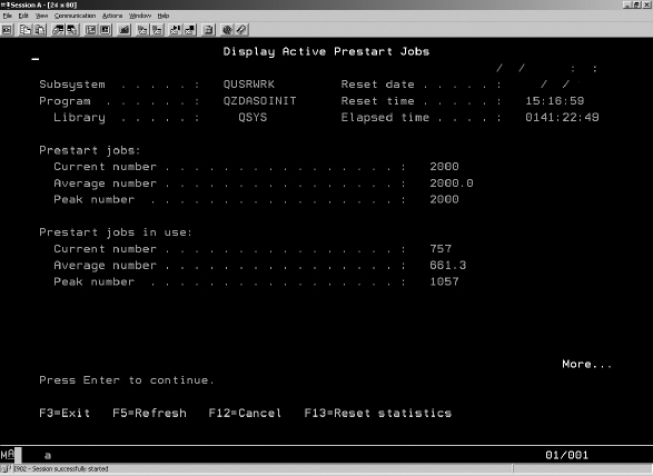
FIGURE 9-4. QUSRWRK/QZDASOINIT prestart allocation usage levels
DSPACTPJ SBS(QUSRWRK) PGM(QZDASOINIT) is issued to review the prestart levels. For QZDASOINIT, we can start 750 or 1000 jobs with a threshold of 50 and allocation of 50 new jobs. This setting matches the actual usage much better than the 2000 allocated jobs, which is significantly higher than the peak usage that wastes resources.Figure 9-5 shows the prestart settings for
QZDASOINIT using the WKRSBS QUSRWRK command and prestart job settings option for the QZDASOINIT entry. The threshold is very low to start additional jobs and could cause delays if more than one user logs in when the 2000 prestart jobs are used. Adding 200 at a time will also create significant delays as well instead of a smaller number like 50. Currently QZDASOINIT runs in shared pool identifier 1 as well, which is planned to change to an appropriate shared memory pool.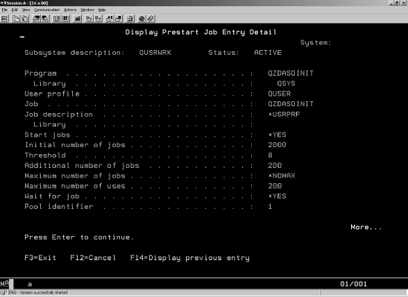
FIGURE 9-5. QZDASOINIT prestart settings set by customer
In Figure 9-6, we issued the
DSPACTPJ SBS(QSYSWRK) PGM(QSQSRVR) command to view the prestart jobs. We recommended 750 to 1000 prestart jobs with a threshold of 50 and allocation of 50 and MAXUSE of 200.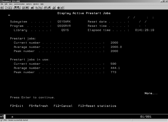
FIGURE 9-6. QSYSWRK/QSQSRVR prestart allocation usage levels
The
MAXUSE parameter was set to 25 instead of the default 200, which causes the overhead of new jobs to be almost 10 times higher than desired. You would be starting a new QSQSRVR database job after 25 uses instead of 200, which for stable connections is much too frequent, increasing overhead unnecessarily.In Figure 9-7, we have similar settings for the QSQSRVR prestart jobs using the using the
WKRSBS QSYSWRK command and prestart job settings option for QSQSRVR entry. We provided similar recommendations in this customer situation due to call object and batch workload present.
FIGURE 9-7. QSQSRVR prestart settings set by customer
The bottom line is to review your prestart settings in use by the JD Edwards EnterpriseOne configuration. You start out with an estimation of the number of users and connections. Over time as you have actual usage, you can adjust the settings to match your average and peak usage based on how the workloads behave. In most cases, once the workload is stable, you do not have to monitor these often, but don’t forget to review them since business processes, code, and configuration changes can influence how many connections are used.
TCP/IP Buffer Size
One change that can benefit larger volume servers connecting to your IBM System i is to consider increasing the network TCP/IP send/receive buffer size. In V6R1 and below, the default buffer size is 8192 bytes, which was useful for slower networks, but not as relevant in the much faster and more reliable networks in use today. The default for V7R1 is 65,536 bytes, but this can also be too low, especially if you have other IBM System i, virtual three-tier or Windows servers connected in the local network to the IBM System i machine. Most customer System i machines utilize 1GB network cards, so changing the TCP/IP attribute can provide improved network throughput. The
CHGTCPA command is dynamic, taking effect immediately, but we generally perform this during low activity levels to be conservative.The command is
Job Class Time Slices
The job class time slices were initially created back in the ’70s and ’80s and have not been adjusted for faster processors—in our opinion—over the years. Generally, after all the other performance tuning has been completed, we examine potentially reducing the time slices by at least a factor of 10 (hundreds instead of thousands) when a customer has thousands of active jobs present in the system. You can consider this for smaller configurations, but you may not observe as significant an improvement versus a system with a large number of active jobs. This allows faster jobs to go through and prevents larger jobs from holding the processor as long. Since you free up the processor time slice sooner, the other smaller eligible jobs get the processor sooner, which can become a cumulative effect. In most situations for busy systems, these changes will result in better performance for JD Edwards EnterpriseOne Web and the batch runtimes when many (thousands or more) active jobs are present.
If a class is already in the hundreds, it should not be changed, and we do not change the time slice values for system parameters that are protected. Basically, the system won’t let you change the system job class parameters.
Use the command
WRKCLS CLS(*ALL/*ALL) to view/edit the entries. An example is shown in Figure 9-8.
FIGURE 9-8. WRKCLS class time slice review and change
When changes are desired, use option 2 to change the entry. Not all system entries can be changed, and those will remain at defaults.
In Figure 9-9, you could change the time slice to 500 milliseconds. Note that these changes do not take effect until the system is recycled or a new job starts, so it is best to coordinate the changes near or within a maintenance window where you IPL the machine.

FIGURE 9-9. Example of JDENET time slice at 5000 milliseconds
There are several opinions regarding this type of change, but we have found that with the newer generations of IBM Power processors, you can observe incremental improvements when you have a high number of concurrent jobs running in your IBM System i. This change is typically one of the later ones that are considered after implementing other recommendations such as the
QAQQINI Optimization_goal, prestart allocations for QZDASOINIT/QSQSRVR and memory pool settings. Changing the job class time slices for busier configurations does skew the configuration to favor shorter jobs such as the queries from web users, but it can also help short-running batch jobs since the longer running jobs do not hold the time slice as long as they previously could. This is a good option to consider once the other areas have been addressed. Do all your other tuning activities before considering this option.Batch Subsystem Priorities
Another option is to divide your batch workloads into different IBM System i subsystems with priorities for the job and memory. You can, for example, use the QBATCH subsystem for most jobs submitted by users and create another batch subsystem such as JDEBATCH at a lower priority such as 60. The QBATCH subsystem typically operates at priority 50, and you could place longer running, more resource-intensive jobs into the JDEBATCH subsystem queues. You would need to modify the queue name in the UBE versions that you want to submit to the JDEBATCH subsystem to match your queue entries. By running at priority 60, these jobs would typically take a little longer than if running at priority 50, but they’d use only leftover resources once the higher priority jobs have their share. Consider this option for UBEs that take perhaps an hour or longer and would be good candidates for this type of batch subsystem configuration. This is a more complex configuration to implement, but it has proven useful when you have a lot of batch activity and want to prioritize certain batches above others.
Memory Pools
In general, there are two primary methods of tuning an IBM System i environment. One option or line of thinking is to allow the machine to manage the resources in a common memory pool. This is the default model used where the bulk of memory management occurs in the *BASE memory pool.
The second option is to allocate shared memory pools, enable the expert cache option, and set priorities as desired for the different jobs/applications. You can then allow the system to dynamically manage the various activity levels, memory, and priorities or you can disable these features and manually tune/monitor them. Our recommendation in the later IBM System i releases is to allocate shared memory pools and allow the system to manage itself with monitoring to ensure the workload goals are being met.
The newer releases of IBM System i have reduced the tuning needs significantly. The move from the Classic Query Engine (CQE) to SQL Query Engine (SQE) provides several advantages to SQL execution and optimizations. IBM System i’s ability to manage the workload dynamically has improved over the years as well. You can use shared memory pools to refine the workload priorities to your business requirements or run generally well in the default *BASE configuration.
Sometimes a compromise exists in that memory can be allocated into several shared pools. A memory pool can be created for the following reasons:
Based on the JD Edwards EnterpriseOne workload criteria, you can create the following suggested pools if you want to separate the workloads:
QZDASOINIT/QSQSRVR jobs that perform the EnterpriseOne ODBC and internal call object/UBE activity. The EnterpriseOne subsystem may also be placed here or in a separate shared pool. Generally the same shared pool as QZDASOINIT/QSQSRVR jobs.Under the
WRKSHRPOOL command you can modify the shared pool sizes and characteristics and then at the subsystem definitions define which jobs go into the specific shared pools. Figure 9-10 shows a shared pool configuration.
FIGURE 9-10. WRKSHRPOOL definitions
Note the memory priority settings has the machine pool at 1 and the rest at 2, minimum size percentages are present, and for this configuration the maximum percentage for *INTERACT was set to limit the memory 5250 terminal users could obtain. In some cases, if you have a low priority batch subsystem, you might set the memory priority to 3.
Figure 9-11 shows the text descriptions of the shared pool purpose to help you understand what jobs/subsystem(s) are in that pool.
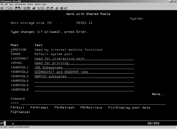
FIGURE 9-11. WRKSHRPOOL descriptions
Figure 9-12 provides an example, where the system has run for a day the dynamic adjustments, and expert cache moves memory between the pools. The JD Edwards EnterpriseOne/
QSQSRVR/QZDASOINIT tend to retain more memory for this particular configuration, and the *BASE and batch subsystems move memory back and forth as the workloads change.
FIGURE 9-12. WRKSHRPOOL example of memory allocations over time
Basically, for shared memory pools the key is to set some minimum memory levels for the EnterpriseOne/
QSQSRVR/QZDASOINIT and batch subsystem to ensure that a certain level of response is maintained. The priority has been changed to 1 for *MACHINE and 2 for all other pools. Minimum memory percentages have been set to ensure a certain amount of memory in that pool is always reserved. You can adjust over time by monitoring the paging and response time of the jobs in that shared pool. The *CALC expert cache is enabled for all the shared pools to manage the pool if dynamic adjustments are allowed.If too much memory is removed from the pool, it can increase the paging rates to bring back either data or programs. We generally start with a value of 5 or 10 percent and then monitor the general response and paging rates of that memory pool. We like to see relatively low paging rates for the EnterpriseOne/
QSQSRVR/QZDASOINIT pool, and for the batch you can usually endure higher paging rates. This does depend on the batch job mix and the turnaround time needed by the business. If you have some really high priority batch jobs that need quick turnaround along with large long-running batch, you may need to separate them into different subsystems and pools, but this is an exception rather than the rule. Note that if you are relatively low on memory, the use of shared pools becomes even more valuable, since you are prioritizing the workload pools and reserving certain resources in those pools.The shared memory pool strategy is very flexible, and we only touched on it in this section. To set up the pools properly takes some initial time and monitoring, but it can allow the IBM System i to adjust itself when workload demands change. There is definitely no one strategy for all customers when it comes to workload management.
Table 9-14 lists some of the performance system parameters that should be reviewed and evaluated. The goal is to allow the IBM System i to manage the memory pools, priorities, and activity levels of the configuration. Each configuration is different in the business processing goals, but the capabilities of the IBM V6R1, V7R1, and later OS (with cumulative patches applied to be as current as possible) work very well. Older OS releases provided more opportunities to tune manually, and you have that option as well, but in our opinion for most JD Edwards EnterpriseOne customers, one of the goals utilizing the IBM System i is to minimize manual management and tuning tasks.
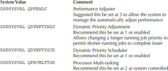
TABLE 9-14. Performance System Parameters to Consider
With a properly sized hardware configuration and well-defined business process workload goals in place, the IBM System i is an excellent platform to operate. As stated previously, you can set the configuration to be fairly static if desired, but that strategy tends to work better in older releases of IBM System i and JD Edwards OneWorld, where you would tend to have a larger number of interactive 5250 users, possibly coexisting with World on the older OS releases. With JD Edwards EnterpriseOne, the workload is heavily skewed toward batch since Web and UBEs are both batch requests with different priority levels. This is why using shared memory pools with dynamic performance adjustments tends to be utilized more often than in the past. Not everyone will agree with dynamic performance adjustments, but our experience has demonstrated that for JD Edwards EnterpriseOne workloads this configuration can be very effective. As with all the tuning recommendations we have provided, you need to verify and evaluate in your particular environment.
..................Content has been hidden....................
You can't read the all page of ebook, please click here login for view all page.