5.2.1 The Simple Rankine Cycle

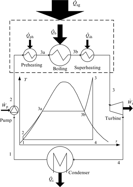
The most basic vapor power cycle is the simple Rankine cycle. This thermodynamic cycle can be described as an ideal internally reversible cycle or as an actual cycle with four irreversible processes. The ideal cycle can be executed with a machine comprising the following components: an ideal pump that operates isentropically and adiabatically (no heat transfer, only work input), an ideal heat exchanger system which plays the role of vapor generator (with no pressure drops and heat losses), a turbine able to operate isentropically and adiabatically (no heat transfer, only work output), and a condenser with no pressure losses and an infinite heat transfer surface (or equivalently an infinite heat transfer coefficient with zero temperature difference between working fluid and heat sink). The vapor generator consists of a preheating section, boiling section, and vapor superheating section. When the working fluid is steam—which is the case for any conventional type of steam power plant—the system is denoted as “steam Rankine cycle.” Note that when an organic fluid or another type of working fluid is used the allure of the T–s diagram might be quite different, depending on the type of the fluid.

The basic configuration (four-components) of the ideal Rankine cycle and the cycle's T–s diagram are presented in Figure 5.1. The cycle comprises four processes: (i) isentropic pressurization of the working fluid in saturated liquid state, process 1–2, (ii) isobaric vapor generation, process 2–3 (with sub-processes of heating 2–3a, boiling 3a–3b and superheating 3b–3), (iii) isentropic expansion of the superheated working fluid, and (iv) a condensation process of the working fluid until it reaches saturated liquid state, process 4–1.

The ideal Rankine cycle is internally reversible but it is not a totally reversible cycle because the heat addition process at the source side is not isothermal. Therefore, the cycle as shown in Figure 5.1 has external irreversibility due to heat transfer at the source side. The heat transfer irreversibilities in this case are determined by the temperature difference T₃ − T, where T represents the temperature of the working fluid which increases along the process 2–3a–3b–3. This involves a heat transfer with finite temperature difference between the heat source and working fluid. As the cycle is not externally reversible, an exergy efficiency smaller than 1 must be assigned to the cycle. The thermodynamic analysis can be pursued according to first and second laws.

The mass and energy balance equations for each of the components and the overall balances for the ideal cycle are given in Table 5.1. For the case of the ideal Rankine cycle there are no exergy destructions in condenser, pump, or turbine. However, provided that the heat source is at constant temperature, the externally irreversible Rankine cycle shows exergy destructions in the vapor generator which can be estimated based on the temperature difference between heat source and working fluid.

Table 5.1

Mass and Energy Balance Equations for the Ideal Rankine Cycle

Comp.	Balance equations	Comp.		Balance equations
Pump (1–2)	MBE: ${\dot{\mathit{m}}}_1={\dot{\mathit{m}}}_2=\dot{\mathit{m}}$ EBE: ${\dot{\mathit{W}}}_{\mathrm{p}}=\dot{\mathit{m}}\left({\mathit{h}}_2-{\mathit{h}}_1\right)$	Vapor generator (2 – 3)	Preheating (2 – 3a)	MBE: ${\dot{\mathit{m}}}_2={\dot{\mathit{m}}}_{3\mathit{a}}=\dot{\mathit{m}}$ EBE: ${\dot{\mathit{Q}}}_{\mathrm{ph}}={\dot{\mathit{m}}}_{3\mathrm{a}}\left({\mathit{h}}_{3\mathrm{a}}-{\mathit{h}}_2\right)$
Turbine (3–4)	MBE: ${\dot{\mathit{m}}}_3={\dot{\mathit{m}}}_4=\dot{\mathit{m}}$ EBE: ${\dot{\mathit{W}}}_{\mathrm{t}}=\dot{\mathit{m}}\left({\mathit{h}}_4-{\mathit{h}}_3\right)$		Boiling (3a-3b)	MBE: ${\dot{\mathit{m}}}_{3\mathrm{a}}={\dot{\mathit{m}}}_{3\mathrm{b}}=\dot{\mathit{m}}$ EBE: ${\dot{\mathit{Q}}}_{\mathrm{b}}=\dot{\mathit{m}}\left({\mathit{h}}_{3\mathrm{b}}-{\mathit{h}}_{3\mathrm{a}}\right)$
Condenser (4–1)	MBE: ${\dot{\mathit{m}}}_4={\dot{\mathit{m}}}_1=\dot{\mathit{m}}$ EBE: ${\dot{\mathit{Q}}}_{\mathrm{c}}=\dot{\mathit{m}}\left({\mathit{h}}_4-{\mathit{h}}_1\right)$		Superheating (3b – 3)	MBE: ${\dot{\mathit{m}}}_{3\mathrm{b}}={\dot{\mathit{m}}}_3=\dot{\mathit{m}}$ EBE: ${\dot{\mathit{Q}}}_{\mathrm{sh}}=\dot{\mathit{m}}\left({\mathit{h}}_3-{\mathit{h}}_{3\mathrm{b}}\right)$
Overall cycle	EBE: ${\dot{\mathit{W}}}_{\mathrm{p}}+{\dot{\mathit{Q}}}_{\mathrm{sg}}={\dot{\mathit{Q}}}_{\mathrm{c}}+{\dot{\mathit{W}}}_{\mathrm{t}}$, where ${\dot{\mathit{Q}}}_{\mathrm{sg}}={\dot{\mathit{Q}}}_{\mathrm{sh}}+{\dot{\mathit{Q}}}_{\mathrm{b}}+{\dot{\mathit{Q}}}_{\mathrm{sh}}=\dot{\mathit{m}}\left({\mathit{h}}_3-{\mathit{h}}_2\right)$

Let us denote the temperature of the heat source T_so. When the ideal Rankine cycle is analyzed, the heat source can be considered at a constant temperature which is equal to the highest temperature of the working fluid. The heat source T_so provides heat input to the processes of preheating, boiling and superheating.

In other words, the vapor generator is assumed with an “infinite surface for heat transfer” which assures that the working fluid reaches the heat source temperature level in the thermodynamic state 3 (see the cycle in Figure 5.1); T₃ = T_so. On the other hand the condensation temperature ideally must be equal to the sink temperature; T₁ = T₄ = T_si.

In addition, the sink temperature is ideally the same as the reference temperature; T_si = T₀. The mass flow rate is the same for all system state points, hence it can be denoted generally with $\dot{\mathit{m}}={\dot{\mathit{m}}}_1={\dot{\mathit{m}}}_2=\dots$. Furthermore, there is no entropy generation or exergy destruction in the condenser, pump or turbine. For the vapor generator the integrals in EnBE and ExBE can be solved directly because T_so = const. For the overall cycle the net power is:

${\dot{\mathit{W}}}_{\mathrm{net}}={\dot{\mathit{W}}}_{\mathrm{t}}-{\dot{\mathit{W}}}_{\mathrm{p}}$

and total heat input is:

${\dot{\mathit{Q}}}_{\mathrm{vg}}={\dot{\mathit{Q}}}_{\mathrm{sh}}+{\dot{\mathit{Q}}}_{\mathrm{b}}+{\dot{\mathit{Q}}}_{\mathrm{sh}}=\dot{\mathit{m}}({\mathit{h}}_3-{\mathit{h}}_2)$

In Chapter 1 three general efficiency definitions that can be applied to Rankine cycles were given. The energy efficiency definition was given in Equation (1.67) and the exergy efficiency definition given either by Equation (1.68) or (1.69), which are equivalent. From Equations (5.1) and (5.2) the energy efficiency of the cycle can be defined in terms of net work output divided by the total heat input at source side (vapor generator), namely

$\mathit{\eta }=\frac{{\dot{\mathit{W}}}_{\mathrm{net}}}{{\dot{\mathit{Q}}}_{\mathrm{in}}}=\frac{{\dot{\mathit{W}}}_{\mathrm{t}}-{\dot{\mathit{W}}}_{\mathrm{p}}}{{\dot{\mathit{Q}}}_{\mathrm{vg}}}$

The exergy efficiency in Equation (1.68) expresses the ratio between the net exergy delivered (net work output) and the actual exergy consumed. In the Rankine cycle the exergy consumed is the same as the exergy delivered by the heat source. Therefore, the exergy efficiency is given by

$\mathit{\psi }=\frac{{\dot{\mathit{W}}}_{\mathrm{net}}}{\dot{\mathit{E}}{\mathit{x}}_{\mathrm{in}}}=\frac{{\dot{\mathit{W}}}_{\mathrm{t}}-{\dot{\mathit{W}}}_{\mathrm{p}}}{\dot{\mathit{E}}{\mathit{x}}_{\mathrm{so}}}$

The exergy efficiency when the heat source is of constant temperature is:

$\mathit{\psi }=\frac{{\dot{\mathit{W}}}_{\mathrm{net}}}{\left(1-\frac{{\mathit{T}}_0}{{\mathit{T}}_{\mathrm{so}}}\right){\dot{\mathit{Q}}}_{\mathrm{so}}}=\frac{\mathit{\eta }}{{\mathit{\eta }}_{\mathrm{C}}}$

where η_C is the Carnot factor of the constant temperature heat source, η_C = 1 − T₀/T_so.

The specific exergy of the flow represents a thermomechanical exergy calculated based on the specific enthalpy and entropy of the working fluid at a given thermodynamic state. According to its definition (see Chapter 1), the exergy is calculated with

$\mathit{e}\mathit{x}=\mathit{h}-{\mathit{h}}_0-{\mathit{T}}_0\left(\mathit{s}-{\mathit{s}}_0\right)$

Here, index 0 represents the reference state which is assumed to be that of water at T₀ = 25 ° C and P₀ = 101.325 kPa. The variation of specific exergy Δex for any process is calculated with:

$\mathrm{\Delta }\mathit{e}\mathit{x}=\frac{\mathrm{\Delta }\dot{\mathit{E}}\mathit{x}}{\dot{\mathit{m}}}={\mathit{ex}}_{\mathrm{out}}-{\mathit{ex}}_{\mathrm{in}}$

where $\dot{\mathit{m}}$ is a reference mass flow rate and subscripts “out” and “in” refer to outlet and inlet conditions, respectively. For each process within the ideal Rankine cycle either heat or work is exchanged between the working fluid and the surroundings. Processes that exchange work with the surroundings are the pumping and the expansion; the specific work is determined with:

$\mathit{w}=\frac{\dot{\mathit{W}}}{\dot{\mathit{m}}}={\mathit{h}}_{\mathrm{out}}-{\mathit{h}}_{\mathrm{in}}$

Here, w is the mass-specific work. Similarly, the heat exchange processes that occur in the preheater, boiler, superheater, and condenser are described by the following equation, which expresses the mass-specific heat flux:

$\mathit{q}=\frac{\dot{\mathit{Q}}}{\dot{\mathit{m}}}={\mathit{h}}_{\mathrm{out}}-{\mathit{h}}_{\mathrm{in}}$

Note that if heat or work is transferred out of the cycle then the sign is negative, whereas if heat or work is received by the working fluid the amount has a positive sign. Thus the work of the pump is negative, and that of the turbine is positive. Heat transfer at the preheater, boiler, and superheater is positive, whereas at the condenser it is negative.

In thermodynamic state 2 the working fluid must have the same specific entropy as in state 1 and the same pressure as in state 3. In thermodynamic state 3a the liquid is saturated at the specified boiling temperature T_b. In state 3b there is a saturated vapor at temperature T_b. State 3 is superheated vapor with the temperature equal to T_b + ΔT_sh. State 4 represents the expanded working fluid at pressure equal to P₁, with the same specific entropy as in state 3. The vapor quality x (required for state 4) is related to specific enthalpy at the state point based on the equation

$\mathit{h}=\left(1-\mathit{x}\right){\mathit{h}}_{\mathrm{l}}+\mathit{x}{\mathit{h}}_{\mathrm{v}}$

where h_l and h_v are the specific enthalpies of saturated liquid and vapor, respectively, at the pressure corresponding to the thermodynamic state.

The mass, energy, entropy and exergy balance equations for the actual Rankine cycle are given in Table 5.2. Some important parameters are defined in Table 5.3. The back work ratio (BWR) represents the ratio of the work required to turn the pump to the work delivered by the turbine. As observed, in the Rankine cycle the BWR is extremely low; below 1%. This is very favorable for high efficiency of power generation. The work necessary to pressurize liquid (pump work) is negligible with respect to the work generated by expansion of gas (turbine work). In this respect, it is an advantage of the Rankine cycle to operate with a working fluid that changes the phase from subcooled liquid to superheated vapor. Other types of thermodynamic cycles that operate with gas have a BWR higher than 30%.

Table 5.2

Balance Equations for the actual Rankine Cycle of Basic Configuration

Component	Balance equations	Component		Balance equations
Pump (1–2)	MBE: ${\dot{\mathit{m}}}_1={\dot{\mathit{m}}}_2$ EBE: ${\dot{\mathit{m}}}_1{\mathit{h}}_1+{\dot{\mathit{W}}}_{\mathrm{p}}={\dot{\mathit{m}}}_2{\mathit{h}}_2$ EnBE: ${\dot{\mathit{m}}}_1{\mathit{s}}_1+{\dot{\mathit{S}}}_{\mathrm{g}}={\dot{\mathit{m}}}_2{\mathit{s}}_2$ ExBE: ${\dot{\mathit{m}}}_1\mathit{e}{\mathit{x}}_1+{\dot{\mathit{W}}}_{\mathrm{p}}={\dot{\mathit{m}}}_2\mathit{e}{\mathit{x}}_2+\dot{\mathit{E}}{\mathit{x}}_{\mathrm{d}}$	Vapor generator (2–3)	Preheating section (2–3a)	MBE: ${\dot{\mathit{m}}}_2={\dot{\mathit{m}}}_{3\mathit{a}}$ EBE: ${\dot{\mathit{m}}}_2{\mathit{h}}_2+{\dot{\mathit{Q}}}_{\mathrm{ph}}={\dot{\mathit{m}}}_{3\mathrm{a}}{\mathit{h}}_{3\mathrm{a}}$ EnBE: ${\dot{\mathit{m}}}_2{\mathit{s}}_2+{\displaystyle \underset{2}{\overset{3\mathrm{a}}{\int }}}\frac{\mathrm{d}{\dot{\mathit{Q}}}_{\mathrm{ph}}}{{\mathit{T}}_{\mathrm{so}}}+{\dot{\mathit{S}}}_{\mathrm{g}}={\dot{\mathit{m}}}_{3\mathrm{a}}{\mathit{s}}_{3\mathrm{a}}$ ExBE: ${\dot{\mathit{m}}}_2\mathit{e}{\mathit{x}}_2+{\displaystyle \underset{2}{\overset{3\mathrm{a}}{\int }}}\left(1-\frac{{\mathit{T}}_0}{{\mathit{T}}_{\mathrm{so}}}\right)\mathrm{d}{\dot{\mathit{Q}}}_{\mathrm{ph}}={\dot{\mathit{m}}}_{3\mathrm{a}}\mathit{e}{\mathit{x}}_{3\mathrm{a}}+\dot{\mathit{E}}{\mathit{x}}_{\mathrm{d}}$
Turbine (3–4)	MBE: ${\dot{\mathit{m}}}_3={\dot{\mathit{m}}}_4$ EBE: ${\dot{\mathit{m}}}_3{\mathit{h}}_3={\dot{\mathit{m}}}_4{\mathit{h}}_4+{\dot{\mathit{W}}}_{\mathrm{t}}$ EnBE: ${\dot{\mathit{m}}}_3{\mathit{s}}_3+{\dot{\mathit{S}}}_{\mathrm{g}}={\dot{\mathit{m}}}_4{\mathit{s}}_4$ ExBE: ${\dot{\mathit{m}}}_3\mathit{e}{\mathit{x}}_3={\dot{\mathit{m}}}_4\mathit{e}{\mathit{x}}_4+{\dot{\mathit{W}}}_{\mathrm{t}}+\dot{\mathit{E}}{\mathit{x}}_{\mathrm{d}}$		Boiling section (3a–3b)	MBE: ${\dot{\mathit{m}}}_{3\mathrm{a}}={\dot{\mathit{m}}}_{3\mathrm{b}}$ EBE: ${\dot{\mathit{m}}}_{3\mathrm{a}}{\mathit{h}}_{3\mathrm{a}}+{\dot{\mathit{Q}}}_{\mathrm{b}}={\dot{\mathit{m}}}_{3\mathrm{b}}{\mathit{h}}_{3\mathrm{b}}$ EnBE:${\dot{\mathit{m}}}_{3\mathrm{a}}{\mathit{s}}_{3\mathrm{a}}+{\displaystyle \underset{3\mathrm{a}}{\overset{3\mathrm{b}}{\int }}}\frac{\mathrm{d}{\dot{\mathit{Q}}}_{\mathrm{b}}}{{\mathit{T}}_{\mathrm{so}}}+{\dot{\mathit{S}}}_{\mathrm{g}}={\dot{\mathit{m}}}_{3\mathrm{b}}{\mathit{s}}_{3\mathrm{b}}$ ExBE: ${\dot{\mathit{m}}}_{3\mathrm{a}}\mathit{e}{\mathit{x}}_{3\mathrm{a}}+{\displaystyle \underset{3\mathrm{a}}{\overset{3\mathrm{b}}{\int }}}\left(1-\frac{{\mathit{T}}_0}{{\mathit{T}}_{\mathrm{so}}}\right)\mathrm{d}{\dot{\mathit{Q}}}_{\mathrm{b}}={\dot{\mathit{m}}}_{3\mathrm{b}}\mathit{e}{\mathit{x}}_{3\mathrm{b}}+\dot{\mathit{E}}{\mathit{x}}_{\mathrm{d}}$
Condenser (4–1)	MBE: ${\dot{\mathit{m}}}_4={\dot{\mathit{m}}}_1$ EBE: ${\dot{\mathit{m}}}_4{\mathit{h}}_4={\dot{\mathit{m}}}_1{\mathit{h}}_1+{\dot{\mathit{Q}}}_{\mathrm{c}}$ EnBE: ${\dot{\mathit{m}}}_4{\mathit{s}}_4+{\dot{\mathit{S}}}_{\mathrm{g}}={\dot{\mathit{m}}}_1{\mathit{s}}_1+{\displaystyle \underset{4}{\overset{1}{\int }}}\frac{\mathrm{d}{\dot{\mathit{Q}}}_{\mathrm{c}}}{{\mathit{T}}_{\mathrm{si}}}$ ExBE: ${\dot{\mathit{m}}}_4\mathit{e}{\mathit{x}}_4={\dot{\mathit{m}}}_1\mathit{e}{\mathit{x}}_1+{\displaystyle \underset{4}{\overset{1}{\int }}}\left(1-\frac{{\mathit{T}}_0}{{\mathit{T}}_{\mathrm{si}}}\right)\mathrm{d}{\dot{\mathit{Q}}}_{\mathrm{c}}+\dot{\mathit{E}}{\mathit{x}}_{\mathrm{d}}$		Superheating section (3b–3)	MBE: ${\dot{\mathit{m}}}_{3\mathrm{b}}={\dot{\mathit{m}}}_3$ EBE: ${\dot{\mathit{m}}}_{3\mathrm{b}}{\mathit{h}}_{3\mathrm{b}}+{\dot{\mathit{Q}}}_{\mathrm{sh}}={\dot{\mathit{m}}}_3{\mathit{h}}_3$ EnBE: ${\dot{\mathit{m}}}_{3\mathrm{b}}{\mathit{s}}_{3\mathrm{b}}+{\displaystyle \underset{3\mathrm{b}}{\overset{3}{\int }}}\frac{\mathrm{d}{\dot{\mathit{Q}}}_{\mathrm{sh}}}{{\mathit{T}}_{\mathrm{so}}}+{\dot{\mathit{S}}}_{\mathrm{g}}={\dot{\mathit{m}}}_3{\mathit{s}}_3$ ExBE: ${\dot{\mathit{m}}}_{3\mathrm{b}}\mathit{e}{\mathit{x}}_{3\mathrm{b}}+{\displaystyle \underset{3\mathrm{b}}{\overset{3}{\int }}}\left(1-\frac{{\mathit{T}}_0}{{\mathit{T}}_{\mathrm{so}}}\right)\mathrm{d}{\dot{\mathit{Q}}}_{\mathrm{sh}}={\dot{\mathit{m}}}_3\mathit{e}{\mathit{x}}_3+\dot{\mathit{E}}{\mathit{x}}_{\mathrm{d}}$
Overall cycle	MBE: there is no MBE because no mass crosses the boundary of the overall system. $\mathrm{EBE}:{\dot{\mathit{W}}}_{\mathrm{p}}+{\dot{\mathit{Q}}}_{\mathrm{sh}}+{\dot{\mathit{Q}}}_{\mathrm{b}}+{\dot{\mathit{Q}}}_{\mathrm{sh}}={\dot{\mathit{Q}}}_{\mathrm{c}}+{\dot{\mathit{W}}}_{\mathrm{t}};\mathrm{EnBE}:{\displaystyle \underset{2}{\overset{3\mathrm{a}}{\int }}}\frac{\mathrm{d}{\dot{\mathit{Q}}}_{\mathrm{ph}}}{{\mathit{T}}_{\mathrm{so}}}+{\displaystyle \underset{3\mathrm{a}}{\overset{3\mathrm{b}}{\int }}}\frac{\mathrm{d}{\dot{\mathit{Q}}}_{\mathrm{b}}}{{\mathit{T}}_{\mathrm{so}}}+{\displaystyle \underset{3\mathrm{b}}{\overset{3}{\int }}}\frac{\mathrm{d}{\dot{\mathit{Q}}}_{\mathrm{sh}}}{{\mathit{T}}_{\mathrm{so}}}+{\dot{\mathit{S}}}_{\mathrm{g}}={\displaystyle \underset{4}{\overset{1}{\int }}}\frac{\mathrm{d}{\dot{\mathit{Q}}}_{\mathrm{c}}}{{\mathit{T}}_{\mathrm{c}}}$ $\mathrm{ExBE}:{\dot{\mathit{W}}}_{\mathrm{p}}+\dot{\mathit{E}}{\mathit{x}}_{\mathrm{so}}={\dot{\mathit{W}}}_{\mathrm{t}}+{\displaystyle \underset{4}{\overset{1}{\int }}}\left(1-\frac{{\mathit{T}}_0}{{\mathit{T}}_{\mathrm{si}}}\right)\mathrm{d}{\dot{\mathit{Q}}}_{\mathrm{c}}+\dot{\mathit{E}}{\mathit{x}}_{\mathrm{d}}$ $\mathrm{where}\dot{\mathit{E}}{\mathit{x}}_{\mathrm{so}}={\displaystyle \underset{2}{\overset{3\mathrm{a}}{\int }}}\left(1-\frac{{\mathit{T}}_0}{{\mathit{T}}_{\mathrm{so}}}\right)\mathrm{d}{\dot{\mathit{Q}}}_{\mathrm{ph}}+{\displaystyle \underset{3\mathrm{a}}{\overset{3\mathrm{b}}{\int }}}\left(1-\frac{{\mathit{T}}_0}{{\mathit{T}}_{\mathrm{so}}}\right)\mathrm{d}{\dot{\mathit{Q}}}_{\mathrm{b}}+{\displaystyle \underset{3\mathrm{b}}{\overset{3}{\int }}}\left(1-\frac{{\mathit{T}}_0}{{\mathit{T}}_{\mathrm{so}}}\right)\mathrm{d}{\dot{\mathit{Q}}}_{\mathrm{sh}}$

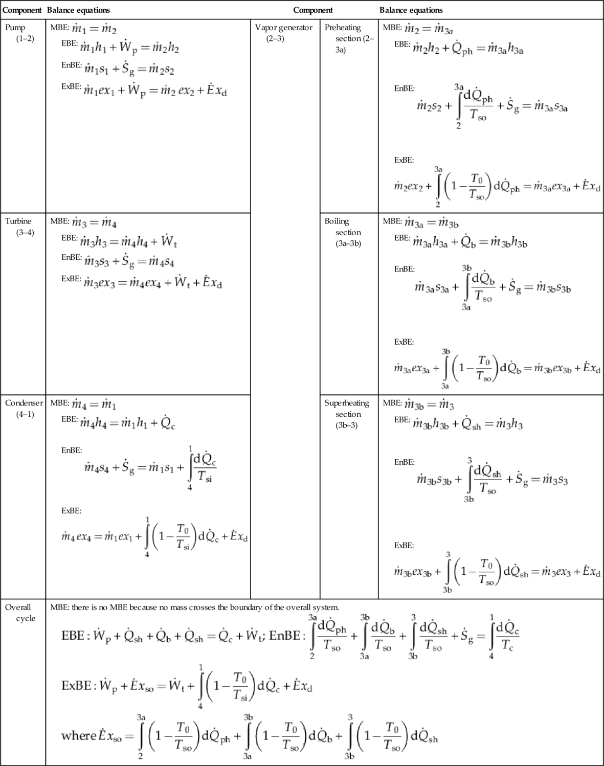
Note: MBE, mass balance equation; EBE, energy balance equation; EnBE, entropy balance equation; ExBE, exergy balance equation; T_so temperature at heat source [K]; T_si temperature at heat sink [K].

Table 5.3

Summary of Important Parameters for the Rankine Cycle

Quantity	Definition	Unit
Heat input	${\dot{\mathit{Q}}}_{\mathrm{in}}={\dot{\mathit{Q}}}_{\mathrm{ph}}+{\dot{\mathit{Q}}}_{\mathrm{b}}+{\dot{\mathit{Q}}}_{\mathrm{sh}}$	kW
Net work output	${\dot{\mathit{W}}}_{\mathrm{net}}={\dot{\mathit{W}}}_{\mathrm{t}}-{\dot{\mathit{W}}}_{\mathrm{p}}$	kW
Energy efficiency, Equation (1.67)	$\mathit{\eta }=\frac{{\dot{\mathit{W}}}_{\mathrm{net}}}{{\dot{\mathit{Q}}}_{\mathrm{in}}}$	%
Exergy delivered	$\dot{\mathit{E}}{\mathit{x}}_{\mathrm{deliv}}={\dot{\mathit{W}}}_{\mathrm{net}}$	kW
Exergy efficiency, Equation (1.68)	$\mathit{\psi }=\frac{\dot{\mathit{E}}{\mathit{x}}_{\mathrm{deliv}}}{\dot{\mathit{E}}{\mathit{x}}_{\mathrm{cons}}}$	%
Carnot factor	${\mathit{\eta }}_{\mathrm{C}}=1-\frac{{\mathit{T}}_0}{{\mathit{T}}_3}$	%
Exergy efficiency (ideal maximum)	$\mathit{\psi }=\frac{{\dot{\mathit{W}}}_{\mathrm{net}}}{{\dot{\mathit{W}}}_{\mathrm{rev}}}=\frac{\mathit{\eta }}{{\mathit{\eta }}_{\mathrm{C}}}$	%
Back work ratio	$\mathit{BWR}=\frac{{\dot{\mathit{W}}}_{\mathrm{p}}}{{\dot{\mathit{W}}}_{\mathrm{t}}}$	%
Pressure ratio	$\mathit{PR}=\frac{{\mathit{P}}_2}{{\mathit{P}}_1}$	-
Expansion ratio	$\mathit{ER}=\frac{{\mathit{v}}_4}{{\mathit{v}}_3}$	-

The pressure ratio (PR) quantifies the ratio between high and low pressure of the Rankine cycle (see Table 5.3). In the steam Rankine cycle the value of PR is quite high due to the fact that steam expands in vacuum. Hence, it is necessary to use a turbine with multiple expansion stages to make the actual expansion process more efficient. Moreover, the parameter ER (expansion ratio) compares the vapor specific volume at turbine exit to the volume at turbine inlet (see Table 5.3). In the Rankine cycle the volume of expanded flow is more than one hundred times larger than the steam volume at the turbine inlet. The expansion ratio is a crucial parameter for turbine design and also quantifies the measure in which the size of low-pressure steam pipes at the turbine outlet must be larger than the high-pressure steam pipes at the turbine inlet.

Example 5.1

We consider in internally reversible Rankine cycle of basic configuration with condensation temperature equal to the reference temperature of T_c = 25 °C and boiling occurring at T_b = 200 °C while the superheating degree is ΔT_sh = 200 °C. The cycle will be analysed thermodynamically according to energy and exergy.

Given that this is an ideal Rankine cycle, it is implicit that all internal processes and the heat transfer process at the condenser are reversible. The thermodynamic states 1–4 of the ideal Rankine cycle can be easily determined from the known parameters T_c, T_b, and ΔT_sh.

In Table 5.4 the calculation steps for the parameters in each of the thermodynamic states of the cycle are briefly explained. Because the mass flow rate is the same in all state points of the cycle all balance equations can be solved in a mass-specific form; intensive properties are therefore used, such as specific enthalpies, entropies, and volumes.

Table 5.4

Thermodynamic States of Ideal Rankine Cycle for Example 5.1

State	State description	Exemplary case study parameters for cycle represented in Figure 5.1
		P(kPa)	T(K)	v(m3/kg)	x	h(kJ/kg)	s(J/kg.K)	ex(kJ/kg)
1	Saturated liquid at Tc	3.169	298.2	0.001003	0	104.8	0.367	0
2	Subcooled liquid at s2 = s1 and P2 = P3	1554	298.2	0.001002	− 0.38	106.3	0.367	1.555
3a	Saturated liquid at Tb	1554	473.2	0.001156	0	852.4	2.331	162.1
3b	Saturated vapor at Tb	1554	473.2	0.1273	1	2793	6.431	879.7
3	Vapor superheated with ΔTsh	1554	673.2	0.1958	1.238	3255	7.252	1097
4	Two-phase fluid at Tc and s4 = s3	3.169	298.2	36.45	0.841	2157	7.252	0

For the ideal steam Rankine cycle it is assumed that in state 1 the liquid at pump intake is in a saturated state. Thus, based on condensation temperature and a vapor quality x₁ = 0 all other parameters such as specific volume, specific enthalpy, specific entropy, and specific exergy of the working fluid can be determined with the help of a selected equation of the state for steam. A highly accurate equation of the state for water and steam is presented in Wagner and Pruss (1993); tabular steam data can be also found in many thermodynamic textbooks, such as Cengel and Boles (2010) or Moran et al. (2011). The Engineering Equation Solver software has implemented advanced equations of state for thermophysical and thermochemical properties of many other substances; this software was used to calculate numerical data within this book (see Klein, 2012).

Note that the vapor quality is by definition a quantity ranging from 0 (liquid) to 1 (vapor). However, in Table 5.4 the value of x goes beyond this limit in two cases. It is given a negative value for x at state 2; the negative sign indicates a subcooled liquid when h < h_l (x₂ = − 0.38; the magnitude of x₂ is proportional with the degree of subcooling). As well, a value of x superior to 1 at state 3 indicates a superheated vapor when h > h_v (x₃ = 1.24; the magnitude of x₃ is proportional with the degree of superheating).

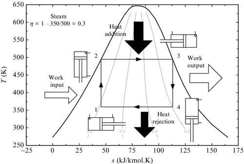
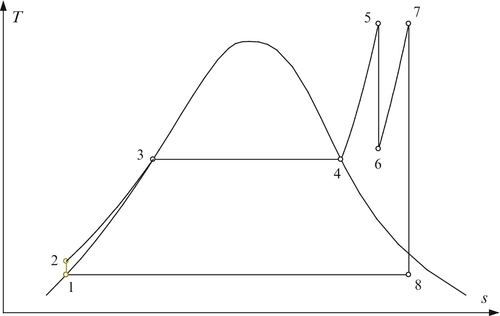
The cycle diagram in T–s coordinates is given in Figure 5.2. As seen, when represented at scale, state 2 confuses with state 1 and the preheating line is superimposed over the saturated liquid line; this behavior is common for steam Rankine cycles. The processes specific to the studied cycle are indicated in Table 5.5. The summary of the calculated cycle parameters are given in Table 5.6. It is remarked that exergy efficiency is 62.5%, whereas the energy efficiency is only 34.8%.

Table 5.5

Processes of Ideal Rankine Cycle from Example 5.1

Process	Process description	Parameters for cycle case study in Example 5.1
		q (kJ/kg)	w (kJ/kg)	Δex (kJ/kg)
1–2	Isentropic pumping s2 = s1, P2 = P3, wp = h2 − h1	N/A	1.555	1.555
2–3a	Isobaric (pre)heating x3a = 0, T3a = Tb, qph = h3a − h2	746.1	N/A	160.6
3a–3b	Isobaric/isothermal boiling x3b = 1, qb = h3b − h3a	1940	N/A	717.6
3b–3	Isobaric superheating P3 = P3b, qsh = h3 − h3b	462.3	N/A	217.7
3–4	Isentropic expansion s4 = s3, P4 = P1, wt = h3 − h4	N/A	1097	1097
4–1	Isobaric/isothermal condensation T4 = T1, qc = h4 − h1	2053	N/A	0.0

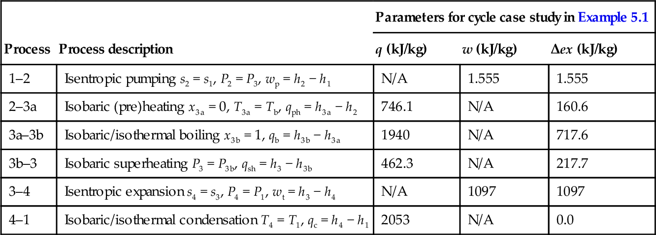
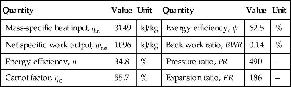
Table 5.6

Summary of Calculated Cycle Parameters for Example 5.1

Quantity	Value	Unit	Quantity	Value	Unit
Mass-specific heat input, qin	3149	kJ/kg	Exergy efficiency, ψ	62.5	%
Net specific work output, wnet	1096	kJ/kg	Back work ratio, BWR	0.14	%
Energy efficiency, η	34.8	%	Pressure ratio, PR	490	–
Carnot factor, ηC	55.7	%	Expansion ratio, ER	186	–

5.2.2 Exergy Destructions in Rankine Power Plants

It is made clear from the above discussion and Example 5.1 that the Rankine cycle is externally irreversible. This is generally valid for any vapor power cycle which includes sensible heating processes such as liquid preheating and vapor superheating because these heat addition processes are non-isothermal. However, it is theoretically possible to imagine a totally reversible vapor power cycle if the heat addition is for a boiling process only.

In Figure 5.3 a totally reversible vapor power generator that operates based on a Carnot cycle (two isothermal and two adiabatic processes) is exemplified. At state 1 a two-phase water-steam mixture at 350 K having a vapor quality of ~0.2 is enclosed in a cylinder and piston assembly. Due to presence of vapor, this mixture is compressible. The piston is moved upward slowly, performing an adiabatic–isentropic compression process (1–2) during which steam liquefies due to pressurization. In state 2 all vapors liquefies and only liquid is found in the cylinder. To perform the compression process a work input to the cycle is required. Further, during process 2–3 heat is added to the working fluid isothermally.

The piston moves freely in order to accommodate the larger volume of vapors formed during heat addition. No work is performed to the outside during process 2–3. In state 3 only saturated vapor is enclosed in the cylinder. There follows an isentropic expansion process (3–4) during which some moisture is formed until the liquid–vapor mixture reaches a vapor quality of 0.8 (as given in the particular example from Figure 5.3).

Work is generated during the piston stroke which compensates for the compression work, and thus a net work output is produced by the cycle. During the last process (4–1) heat is removed isothermally from the cycle and vapor condenses, thus the volume of the cylinder has to reduce. Although it appears theoretically realizable, this kind of engine has never been constructed because of some insurmountable technical obstacles. For example, during the isothermal heat addition the volume of the working fluid must increase about one thousand times, which is unpractical. Also compressing and expanding in two phases must be performed extremely slowly in order to approach isentropic processes. In this section the irreversibilities and exergy destructions in actual vapor power plants are analyzed and methods for their quantification are given.

Each component of an actual power plant destroys exergy. The most important component of a Rankine power station is the steam turbine, which has the role of converting the energy carried by hot, high-pressure steam into useful shaft power which turns the electric generator. The other components of the plant—major and minor—have the sole role of working jointly to provide a continuous stream of steam at the turbine inlet. The major components of a Rankine power station besides the turbine are the steam generator, the pumps, and the condensers. Other important components are feedwater heaters and a preheater, superheater, reheater, and economizer. Minor components are many: separators, steam traps, drum, drains, valves, check valves, safety valves, etc. There are also components specific to various kinds of power stations—depending on the fuel source—coal, oil, natural gas, or nuclear.

More realistic analysis of the Rankine cycle is also necessary to determine the practically attainable efficiency of a given power plant. In this respect the exergy destruction due to water pumping, steam expansion, heat transfer, and fluid flow resistance must be accounted for. The common way in which irreversibilities are accounted for in power plant analysis is by the use of a number of parameters, as follows:

• Isentropic efficiency of turbines—that expresses the ratio of actual work to isentropic (i.e., reversible) work developed by the turbine

• Isentropic efficiency of pumps—that expresses the ratio of the isentropic (i.e., reversible) work to the actual work required by pumps

• Mechanical efficiency—which quantifies the difference between net amount of work developed by the working fluid and the mechanical work developed by the turbine shaft

• Electrical efficiency—which expresses the conversion efficiency of the mechanical power of the turbine shaft to the electrical power delivered to the consumer (e.g., electrical grid)

• Temperature difference at heat exchangers at source side—which quantifies the difference between the exergy extracted from the heat source and that delivered to the working fluid

• Heat losses at source-side heat exchangers and hot steam conduits—which induces exergy losses and a reduction of net exergy delivered by the heat source to the working fluid

• Temperature difference at condenser—which quantifies the exergy difference between that rejected by the working fluid and that received by the heat sink; there are two cases:

• if the heat sink is a lake, then a minimal temperature difference of ~ 10 °C must be assumed between the condensation temperature and the sink temperature

• if the heat sink is air and a cooling tower is used to reject heat then a temperature difference of a minimum 5 °C must be considered between air and cooling water and in addition a minimum temperature difference between cooling water and condensation has to be assumed; there must be at least a 15 °C temperature difference between condensation and the wet bulb temperature

• Subcooling degree—which is a technical requirement at pump inlet to prevent cavitation issues and malfunction; subcooling also leads to exergy losses with respect to ideal cycle

• Pressure drop in heat exchangers and conduits—which quantifies the loss of exergy due to the friction process between the fluid steam and walls (pipes, conduits, tubes, heat transfer surfaces) in which the fluid is confined or with which it comes in contact

• High-pressure steam leakage rate—which cannot be prevented because the turbine cannot be perfectly sealed and thus additional energy is required to supply additional fresh water as working fluid

• Air penetration rates at condenser—which cannot be stopped because the condenser operates in a vacuum; this increases the pressure in the condenser and reduces turbine work. Moreover, energy consumption is required to de-aerate the condenser and maintain a reasonable lower pressure

• Energy consumption for auxiliary equipment and power plant house—several pieces of auxiliary equipment, such as (depending on the case) conveyors, fuel injectors, fans, pumps, blowers, electric motors, and also lighting and requirements for the power plant house, will diminish the net power delivered to the consumer by a conventional power generation station

In Table 1.8 the balance equations and energy and exergy efficiency formulations for all important devices used in the power generation system are introduced. In this section the exergy analysis presented in Chapter 1 will be applied in order to exemplify how the irreversibilities in steam Rankine cycles can be assessed.

There are at least four additional processes that must be represented on an actual basic Rankine plant diagram that are not present on an ideal plant diagram: water subcooling at pump inlet, heat loss at hot steam conduits, high-pressure steam leak at the turbine, and fresh water addition at the condenser.

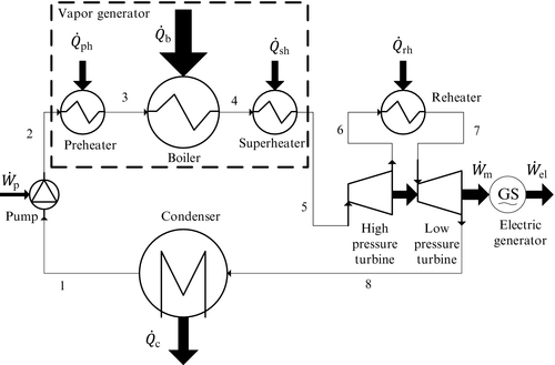
These processes are represented in Figure 5.4, which illustrates an actual steam Rankine cycle of basic configuration. The $\overline{\mathit{T}}$ notations in the figure represent the average system boundary temperature at locations where heat transfer processes occur. In subsequent paragraphs the thermodynamic analysis of the Rankine cycle with irreversibilities is presented and exergy destructions and entropy generations quantified. There are entropy transfer fluxes between surroundings and power plant which can be written mathematically as follows (see Figure 5.4):

${\dot{\mathit{S}}}_{\mathrm{ph}}=+\frac{{\dot{\mathit{Q}}}_{\mathrm{ph}}}{{\mathit{T}}_{\mathrm{ph}}};{\dot{\mathit{S}}}_{\mathrm{b}}=+\frac{{\dot{\mathit{Q}}}_{\mathrm{b}}}{{\mathit{T}}_{\mathrm{b}}};{\dot{\mathit{S}}}_{\mathrm{sh}}=+\frac{{\dot{\mathit{Q}}}_{\mathrm{sh}}}{{\mathit{T}}_{\mathrm{sh}}};{\dot{\mathit{S}}}_{\mathrm{loss}}=-\frac{{\dot{\mathit{Q}}}_{\mathrm{loss}}}{{\mathit{T}}_{\mathrm{loss}}};{\dot{\mathit{S}}}_{\mathrm{c}}=-\frac{{\dot{\mathit{Q}}}_{\mathrm{c}}}{{\mathit{T}}_{\mathrm{c}}};{\dot{\mathit{S}}}_{\mathrm{sc}}=-\frac{{\dot{\mathit{Q}}}_{\mathrm{sc}}}{{\mathit{T}}_{\mathrm{sc}}}$

where the sign indicates that entropy flux enters (+) or exits (−) the thermodynamic cycle.

The thermodynamic analysis of the cycle can start from thermodynamic state 1 where the working fluid is saturated. Three parameters must be specified in order to determine thermodynamic state 1; these are:

• The reference temperature T₀ (which can be the temperature of surrounding atmosphere if the condenser is cooled with air, or the lake temperature if the condenser is cooled with water; T₀ should be the lowest temperature of power plant surroundings)

• The assumed minimum temperature difference at the heat sink (condenser), ΔT_c

• The required subcooling degree ΔT_sc necessary for the pump to operate without cavitation.

Thermodynamic state 1 is completely determined by specifying that the liquid is saturated (x₁ = 0) and that the temperature of working fluid is given by

${\mathit{T}}_1={\mathit{T}}_0+\mathrm{\Delta }{\mathit{T}}_{\mathrm{sc}}+\mathrm{\Delta }{\mathit{T}}_{\mathrm{c}}$

The degree of subcooling in practical applications is taken as ΔT_sc = 1 − 3 °C, whereas ΔT_c = 10 − 15 °C. The condensation pressure is the saturation pressure corresponding to T₁. There is negligible pressure drop in any practical subcooling process. However, some pressure drop must be accounted for across the condensation process. Hence, one can take P₂ = P₁. Further, the temperature of state 2 (subcooled liquid) is determined

${\mathit{T}}_2={\mathit{T}}_1-\mathrm{\Delta }{\mathit{T}}_{\mathrm{sc}}$

State 2 is completely specified because its pressure and temperature can be determined. Thermodynamic state 3 can be determined once the isentropic efficiency of the pump (η_s,p) and the pressure P₃ are specified. The isentropic efficiency allows for determination of specific flow enthalpy and is defined by the following equation (see also Chapter 1):

${\mathit{h}}_{\left({\mathit{P}}_3,{\mathit{s}}_2\right)}-{\mathit{h}}_1={\mathit{\eta }}_{\mathrm{s},\mathrm{p}}\left({\mathit{h}}_2-{\mathit{h}}_1\right)$

The type of pump must be chosen in accordance with the head and the flow rate and economic criteria. For low head, centrifugal pumps of multistage configuration are generally preferred. For high head the preferred choice is of double-casing barrel pumps which are also tolerant to high water temperatures. The acceptable range of isentropic efficiency for pumps at power generating stations is 0.8–0.9.

The pressure in state 3 should be superior to the pressure is state 4 (boiling pressure) due to the existence of pressure drop in preheater. In general the preheater is considered as part of the vapor generator, and, depending on the case, it generally consists of an assembly of pipes heated from the exterior and working fluid circulating internally. In some typical cases (e.g., nuclear power stations) the preheater may be just a part of a shell and tube steam generator which has the hot heat transfer fluid circulating in tubes and water being preheated and boiled in the shell side. In typical power plants the pressure drop over preheaters leads to a decrease in saturation temperature of 0.1–0.3 °C. Denoting ΔT_sat,ph the decrease of saturation temperature due to pressure drop across preheaters, the pressure in state 3 results from the equation

${\mathit{P}}_3={\mathit{P}}_{\mathrm{sat}}\left({\mathit{T}}_{\mathrm{b}}+\mathrm{\Delta }{\mathit{T}}_{\mathrm{sat},\mathrm{ph}}\right)$

The pressure in state 4 corresponds to saturation at a specified boiling temperature that typically is in the range of T_b = 100 − 330 °C, depending on the actual type of power generating station. In state 4 there is a saturated liquid, from which all state parameters can be determined based on temperature T₄ = T_b and vapor quality x₄ = 0. There are many types of boilers, depending on the nature of the heat source. In a coal-fired power plant vertical tubular boilers are used, with boiling occurring in pipes heated by radiation and convection by combustion gases. In oil-fired plants the boilers may be of horizontal return tubular type, again with the boiling process occurring in tubes. Gas-heated power plants have boilers comprising a number of bare or extended-surface tubes forming a heat exchanger register and disposed in a horizontal configuration. In a nuclear power plant the steam generators a pool boiling process is the preferred one.

In any type of boiler there is an unavoidable pressure drop due to working fluid flow. The decrease in saturation temperature due to pressure drop over the boiler (ΔT_sat,?b) is on the order of 0.5–1.5 °C, depending on its actual type. Thus the thermodynamic state 5 at boiler exit is fully determined based on its temperature T₅ = T_b − ΔT_sat,?b and the vapor quality x₅ = 1. The decrease in saturation temperature caused by pressure drop during the superheating process which occurs in superheater or reheater (ΔT_sat,?sh) is in a practical range of 0.3–0.7 °C. In fossil fuel power stations the superheaters are of tubular type (with or without extended surface), with steam circulated in tubes and heat provided from the exterior. In a nuclear power plant, the superheater may be the same unit as the steam generator. Using an assumed ΔT_sat,?sh, the thermodynamic state 6 (Figure 5.4) is determined based on pressure P₆ given by

${\mathit{P}}_6={\mathit{P}}_{\mathrm{sat}}({\mathit{T}}_5-\mathrm{\Delta }{\mathit{T}}_{\mathrm{sat},\mathrm{sh}})$

and on temperature T₆ = T_sh.

The pressure drop in steam conduits of power plants is in the range of ΔP_drop = 0.2 − 0.4 MPa. This pressure drop is due to the high complexity of the steam circuits, which include many types of fittings (screwed, flanged, compensators), headers and manifolds, valves, and check valves.

The steam conduits must be well insulated to minimize the heat losses. It is impossible to avoid heat losses at high-temperature steam conduits because there is generally a considerable distance between the steam generator and the turbine location. In addition, conventional power generating stations have massive steam conduits that must be supported and anchored at many points using special “heat transfer bridges” where heat losses are more accentuated. The temperature reduction of steam due to heat losses at hot steam conduits in power plants can be taken on the order of ΔT_loss = 10 − 30 °C. Hence the thermodynamic state 7 at the turbine inlet is determined based on its pressure and temperature.

The turbine’s irreversibilities are accounted for by specifying the exergy efficiency (η_s,?T). Hence, the specific enthalpy of steam at the turbine outlet results from:

${\mathit{h}}_7-{\mathit{h}}_8={\mathit{\eta }}_{\mathrm{s},\mathrm{T}}\left({\mathit{h}}_7-{\mathit{h}}_{\left({\mathit{P}}_8,{\mathit{s}}_7\right)}\right)$

The isentropic efficiency of the turbine has the highest influence on overall cycle efficiency, hence the correct choice of turbine is crucial for a power plant. After Parson’s invention of the reaction steam turbine—in the last quarter of the nineteenth century—steam turbine technology developed fast in the twentieth century. In the first quarter of the nineteenth century there were many types of proprietary steam turbine designs, such as Parson, Westinghouse-Parson, De Laval, Terry, Kerr, Curtis, Hamilton-Holtzworth, and Allis Chalmers. Steam turbines are generally considered highly reliable equipment in conventional power generation stations. They can be classified as impulse and reaction turbines or as condensing, extraction, reheat, and back pressure (non-condensing) turbines. Reheat and condensing turbines are those which are normally used in conventional Rankine power stations. Modern turbines are conceived as a succession of stages of impulse and reaction blades, with impulse-type of stages at higher pressures and reaction-type stages at lower pressures. The isentropic efficiency of modern steam turbines for conventional power stations spans from 0.8 to 0.9.

The pressure at the turbine outlet (state 8) is practically the same as pressure at the condenser inlet. The number of stages of the turbine can be approximated based on the isentropic nozzle formula that correlates the pressure in the throat (P*) with pressure at the nozzle inlet and the specific heat ratio of the steam, γ. For superheated steam γ = 1.14, while saturated steam is generally approximated with γ = 1.3. The general formula for throat pressure is

${\mathit{P}}^{\mathit{*}}={\left(\frac{2}{\mathit{\gamma }+1}\right)}^{\frac{\mathit{\gamma }}{\mathit{\gamma }-1}}{\mathit{P}}_{\mathrm{in}}$

from which, using the values of γ, it results that

${\mathit{P}}^{\mathit{*}}=\left\{\begin{array}{c}0.546{\mathit{P}}_{\mathrm{in}},\mathit{for}\mathit{superheated}\mathit{steam}\\ 0.576{\mathit{P}}_{\mathrm{in}},\mathit{for}\mathit{saturated}\mathit{steam}\end{array}\right.$

where P_in stands for pressure at the turbine stage inlet.

Moisture does not actually form inside the steam turbine if the vapor quality is higher than 96% because of the character of the flow, which is a fast flow. Hence, the thermodynamic states in the turbine are metastable: there is not sufficient time for heat transfer or for steam condensation to occur. The thermodynamic locus connecting states with steam quality of 96% (or 4% moisture) is known as the Wilson line. If the thermodynamic state in a turbine stage is above the Wilson line, then the steam is dry. If the thermodynamic state is below Wilson line, in that particular stage steam condensation occurs.

The magnitude of pressure drop on the low-pressure steam line and condenser altogether is of 1–2 kPa, which leads to a saturation temperature drop of ΔT_{sat, c} = 2 − 4 °C. The steam condenser is a massive shell-and-tube heat exchanger with steam condensing at the shell side and with water circulating in pipes.

The mechanical efficiency of the power plant is a parameter that accounts for losses caused by turbine friction, steam leak, and any other mechanical losses at the turbine and is defined by

${\mathit{\eta }}_{\mathrm{m}}=\frac{{\mathit{w}}_{\mathrm{m}}}{{\mathit{w}}_{\mathrm{net}}}=0.88-0.94$

In power generation stations the turbines are optimized to rotate synchronously with the power grid—at 3600 RPM in North America, Japan, and South Korea, where the electrical grid is at 60 Hz and at 3000 RPM and where the grid frequency is 50 Hz. The generator, which is connected in line with the turbine shaft is of synchronous type with a copper-coiled rotor and stator. Both the rotor and the stator generate an important amount of heat. For the stator, heat is removed by cooling from the exterior, but for the rotor it is difficult to reject the generated heat because of the small free space between stator and rotor. The current technology for rotor cooling uses hydrogen as a heat transfer fluid. Hence, an enclosure is built around rotor. The generator is linked to a transformer that raises the electric voltage up to over 100 kW in compatibility with the electrical grid. The electrical efficiency, representing the ratio between electrical energy delivered by the generator–transformer assembly and the mechanical energy transferred by the shaft to the generator is defined by

${\mathit{\eta }}_{\mathrm{el}}=\frac{{\mathit{w}}_{\mathrm{el}}}{{\mathit{w}}_{\mathrm{m}}}=0.9-0.96$

There are many auxiliary devices in power plants that consume power, and hence diminish, even if in small measure, the net generation. Here are listed some relatively important auxiliary power-consuming processes and devices of conventional power generation stations:

• If condenser is cooled with water from a lake, there must be installed water circulation pumps and water purification systems which require electrical motors to drive pumps

• If condenser is cooled with hyperboloid cooling tower there must be installed water recirculation pumps and water-feeding pumps driven by electrical motors

• If condenser is cooled by mechanical-draft cooling tower, besides the use of electrically driven pumps there must be installed electrically driven fans for air circulation in forced convection

• In coal-fired power stations there are coal conveyers, ash conveyers, coal mills, and pulverizers that consume power

• In natural gas and oil-fired power station the burners must have blowers driven by electrical motors

• Chimneys when installed require electrically driven fans and blowers

• In fossil fuel plants rotary wheel economizers turned by electric motors are installed at exhaust gases

• Some boilers require additional feed pumps

• Turbine auxiliary parts, such as lubrication system and generator cooling system, require some power consumption

• The power station house requires power for lighting, appliances, alarms, and data acquisition, etc.

For a conventional power generating station, the power consumption for all auxiliary devices and processes, including that for the steam power station house, represents a small fraction of the generated electric power, usually 0.5–1%. Other losses such as those caused by steam leakage and air penetration are small and can be neglected with respect to other more important energy losses.

In Table 5.7 the main parameters which quantify the irreversibilities of steam power stations are summarized. The turbine’s isentropic efficiency influences the cycle efficiency to a very large measure. A change of isentropic efficiency of 10% leads to a change of cycle energy efficiency of ~ 3–4% while exergy efficiency change is 8–9%. Temperature difference between the working fluid and the heat source affects the exergy efficiency. As an order of magnitude, a change of temperature of 50 °C may induce a reverse change of exergy efficiency of 1–2%. Heat losses at hot steam conduit inlets influence the cycle’s energy efficiency, but in very small measure, ~ 0.2%. All other irreversibilities have even smaller influence (independently) on energy efficiency of the cycle.

Certain inequality-type relations must be satisfied between state parameters in order comply with the second law of thermodynamics. More specifically, the energy and entropy balance equations for the subcooler (1–2) require

${\mathit{h}}_1={\mathit{h}}_2+{\mathit{q}}_{\mathrm{sc}}\mathrm{a}\mathrm{n}\mathrm{d}{\mathit{s}}_1+{\mathit{s}}_{\mathrm{gen}}={\mathit{s}}_2+\frac{{\mathit{q}}_{\mathrm{sc}}}{{\overline{\mathit{T}}}_{\mathrm{sc}}}$

As the generated entropy must be positive, from the above equations it results that the following inequality must be satisfied

${\overline{\mathit{T}}}_{\mathrm{sc}}<\frac{{\mathit{h}}_1-{\mathit{h}}_2}{{\mathit{s}}_1-{\mathit{s}}_2}$

which reflects the fact that the cooling medium of the subcooler must have an average temperature ${\overline{\mathit{T}}}_{\mathrm{sc}}$ below a certain value; in addition it is known that ${\overline{\mathit{T}}}_{\mathrm{sc}}>{\mathit{T}}_0$.

The energy and entropy balance on the preheater are

${\mathit{h}}_3+{\mathit{q}}_{\mathrm{ph}}={\mathit{h}}_4\mathrm{a}\mathrm{n}\mathrm{d}{\mathit{s}}_3+\frac{{\mathit{q}}_{\mathrm{ph}}}{{\overline{\mathit{T}}}_{\mathrm{ph}}}+{\mathit{s}}_{\mathrm{gen}}={\mathit{s}}_4$

From the above equation it results that the following inequality must be satisfied

${\overline{\mathit{T}}}_{\mathrm{sh}}>\frac{{\mathit{h}}_4-{\mathit{h}}_3}{{\mathit{s}}_4-{\mathit{s}}_3}$

which states that the average temperature of the heat source temperature at the preheater must be higher than a threshold value that insures that the generated entropy is positive.

Similarly inequalities are derived from the energy and entropy balances on the boiler and superheater as follows:

${\overline{\mathit{T}}}_{\mathrm{b}}>\frac{{\mathit{h}}_5-{\mathit{h}}_4}{{\mathit{s}}_5-{\mathit{s}}_4}\mathrm{a}\mathrm{n}\mathrm{d}{\overline{\mathit{T}}}_{\mathrm{sc}}>\frac{{\mathit{h}}_6-{\mathit{h}}_5}{{\mathit{s}}_6-{\mathit{s}}_5}$

Furthermore, because the preheater, boiler, and superheater are all heated from the same heat source, it results that the following inequalities must be satisfied

${\overline{\mathit{T}}}_{\mathrm{sh}}>{\overline{\mathit{T}}}_{\mathrm{b}}>{\overline{\mathit{T}}}_{\mathrm{ph}}$

The irreversibilities due to heat losses and pressure drop which occurs at conduits that transport hot, high-pressure steam to the turbine are accounted for by specifying the parameters ΔP_drop and ΔT_loss defined in Table 5.7. The energy and entropy balance equations for process 6–7 (see Figure 5.4), which models these types of losses, require that

${\overline{\mathit{T}}}_{\mathrm{loss}}<\frac{{\mathit{h}}_6-{\mathit{h}}_7}{{\mathit{s}}_6-{\mathit{s}}_7}$

The energy and entropy balances for the condenser can be combined to eventually derive the following inequality that must be satisfied

${\overline{\mathit{T}}}_{\mathrm{sc}}<{\overline{\mathit{T}}}_{\mathrm{c}}<\frac{{\mathit{h}}_8-{\mathit{h}}_1}{{\mathit{s}}_8-{\mathit{s}}_1}$

As a conclusion of this section it is clearly noted that the effect of irreversibilities is very important for the steam Rankine cycle and must be quantified accurately in order to predict the actual plant performance. Furthermore, exergy efficiency reveals that the organ which destroys most of the steam exergy is the turbine. Hence, the selection of turbine and its design improvement are crucial issues when designing steam power plants.

The increase of cycle efficiency is very important in practice because it leads to important savings of thermal energy supply (or fuels) and reduction of environmental impact. The engineering goal is to “impinge” the design toward the limits imposed by the second law of thermodynamics. In other words, the design engineer must find ways to reduce the cycle irreversibilities.

In many engineering thermodynamics textbooks some methods to increase the efficiency of the ideal Rankine cycle are discussed. Basic thermodynamic analysis shows that increase of source temperature and/or decrease of sink temperature leads to higher cycle efficiency of any thermodynamic cycle. This is confirmed by a simple analysis of the Carnot factor 1 − T₀/T with a decreasing T₀ and increasing T. Let us assume that T₀ is replaced by T₀ − ΔT and T is replaced with T + ΔT. Figure 5.5 reports Carnot factor η when ΔT is varied from 0 to 50 K. For the reference case (ΔT = 0) it is taken that T₀ = 25 ° C and T = 200 ° C, in which case η_ref = 0.557. Three types of Carnot factors are reported, corresponding to three cases:

• Sink temperature (condensation) is decreased with ΔT, hence η = 1 − (T₀ − ΔT)/T.

• Source temperature is increased with ΔT, hence η = 1 − T₀/(T + ΔT).

• Both source and sink temperatures are changed, hence η = 1 − (T₀ − ΔT)/(T + ΔT).

The results show that it is relatively more important to reduce the sink temperature than to increase the source temperature. If sink temperature decreases by 50 K then efficiency increases by ~ 8%, from 55.7–63.1%. If source temperature is increased with 50 K then the Carnot factor will increase only by 3%. If both temperatures are changed with 50 K then the Carnot factor increases by 10%.

The same trend is observed in the ideal Rankine cycle. In the steam Rankine cycle the condensation temperature is limited by the freezing point of water when working fluid freezes; however, for practical reasons one cannot run water as a working fluid at temperatures lower than 4 − 5 ° C (note that at the bottom of deep lakes and with seawater there is a steady temperature of ~ 4 °C. A simple parametric study is reported in Figure 5.6 which shows the variation of energy efficiency of an ideal steam Rankine cycle when the condensation temperature is decreased by ΔT = 0 … 50 K with respect to a reference value of 55 ° C, and when boiling temperature is increased with same ΔT with respect to a reference value of 175 ° C, and when the temperature of superheated vapor increases from the reference value of 400 ° C with by the amount ΔT; only one parameter is changed at a time while all other cycle parameters remain unchanged.

As seen, the reference cycle efficiency is 27%. If condensation temperature is decreased from 55 to 5 °C the cycle efficiency increases to 36.2% (or a 9.2% increase). If boiling temperature increases from 175 to 225 °C the cycle efficiency reaches 31.9% (that is, a 4.9% increase). Note that in the last case the pressure of the boiler increases from 890 to 2550 kPa, while the highest temperature of the cycle is assumed to be constant, T₅ = 400 ° C. The increase of boiler pressure due to increase of boiling temperature is illustrated in Figure 5.6. If the boiling temperature is 225 °C and condensation is at 5 °C then the cycle efficiency becomes 40% (or a 13% increase with respect to the reference case). The last curve plotted on the graph in Figure 5.6 shows the variation of energy efficiency when the temperature of superheated vapor, T₅, increases from 400 to 450 °C. In this case the cycle efficiency increases relatively less, from 27% to 27.9%.

This simple study suggests a strategy of efficiency improvement for the steam Rankine cycle: first one must set the condensation temperature at the lowest value possible, then one needs to increase the boiling temperature (and pressure) to the highest technical-economic value that is advantageous, and, as a last measure, one must set the temperature of superheated vapor as high as possible based on the practical temperature level that can obtained from the specific heat source considered in the application. Note also that the boiler pressure is limited by technical–economical considerations related to materials selection. For example, in conventional nuclear power plant the boiling pressure is ~5 MPa and the superheated vapor temperature is limited to ~ 350 °C for safety reasons. Furthermore, in a conventional Rankine cycle—which includes a boiling process—the highest pressure should be lower than the critical pressure of steam, which is 22.06 MPa. Newly emerging non-conventional Rankine cycles can operate at supercritical pressure and hence have better efficiency than the conventional cycles.

Example 5.2

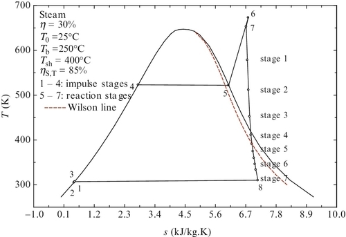
We give an example of the thermodynamic analysis of a Rankine cycle with exergy destructions. The cycle configuration and state points are as shown in Figure 5.4. The assumed parameters for the cycle are given in Table 5.8. It is required to determine the entropy generated and exergy destroyed for each process, the exergy destroyed by the cycle, the exergy wasted, the cycle efficiencies, the BWR and expansion ratio, and the number of turbine stages.

Table 5.8

Performance Parameters of a Non-Ideal Rankine Cycle of Basic Configuration

Assumed parameters		Cycle performance parameters
Parameter	Value	Irreversibilities
T0	25 °C	Component	sgen (J/kg.K)	exd (kJ/kg)	(%)
Tb	250 °C	Subcooler (1–2)	0.193	0.06	0.0
Tsh	400 °C	Pump (2–3)	2.311	0.689	0.2
ηs,T	0.85	Preheater (3–4)	222.8	66.4	17.3
ηs,P	0.85	Boiler (4–5)	276.0	82.3	21.5
ΔTc	7 °C	Superheater (5–6)	71.0	21.2	5.5
ΔTsc	2 °C	Heat lossesa (6–7)	70.0	20.6	5.4
ΔTsat,?ph	0.2 °C	Turbine (7–8)	529.7	157.9	41.2
ΔTsat,?b	1 °C	Condenser (8–1)	113.9	33.9	8.9
ΔTsat,?sh	0.7 °C	Specific energy and exergy flows (kJ/kg)
ΔPdrop	0.3 MPa	qin = qph + qb + qsh			3077
ΔTloss	20 °C	wnet = wt − wp			926.3
ΔTsat, c	3 °C	qwaste = qin − wnet			2151
Tsc	304 K	$\mathit{e}{\mathit{x}}_{\mathrm{in}}={\mathit{q}}_{\mathrm{ph}}\left(1-\frac{{\mathit{T}}_0}{{\mathit{T}}_{\mathrm{ph}}}\right)+{\mathit{q}}_{\mathrm{b}}\left(1-\frac{{\mathit{T}}_0}{{\mathit{T}}_{\mathrm{source},\mathrm{b}}}\right)+{\mathit{q}}_{\mathrm{sh}}\left(1-\frac{{\mathit{T}}_0}{{\mathit{T}}_{\mathrm{sh}}}\right)$			1362
Tph	500 K	$\mathit{e}{\mathit{x}}_{\mathrm{d}}={\displaystyle \sum _{\mathrm{i}}}\mathit{e}{\mathit{x}}_{\mathrm{d},\mathrm{i}}$			383.1
Tsource. b	550 K	exwaste = exd,surr = exin − wnet − exd			52.8
Tsh	600 K	Cycle efficiencies, BWR and ER
Tloss	338 K	η = wnet/qin = 30.1%	${\mathit{\eta }}_{\mathrm{C}}=1-{\mathit{T}}_0/{\stackrel{\mathrm{-}}{\mathit{T}}}_{\mathrm{sh}}=54.1\mathit{\%}$		BWR = 0.5%
Tsink,?c	305K	ψ = η/ηC = 55.6%	ψ = wnet/exin = 68%		ER = 267

^a Heat losses from hot steam conduits (losses due to pressure drop are included).

The mass balance equations require that the mass flow rate is the same at each state point, ${\dot{\mathit{m}}}_{\mathrm{i}}=\dot{\mathit{m}}$. The energy balance equations can be written for each process as indicated in Example 5.1. From energy balances the temperature, pressure, specific volume, specific entropy, and specific enthalpy at each state point can be calculated. From these the specific exergy at each state point can be determined. It is reasonable to assume that the reference state is liquid water at T₀ = 25 °C, P₀ = 101.325 kPa. Entropy and exergy balance equations give the entropy generated and exergy destroyed for each component, respectively. In Table 5.8 the relevant equations are given together with the results.

It is remarked that the maximum exergy destruction is at the turbine at 41.2%, which is assumed to operate with an isentropic efficiency of 85% per stages (see Table 5.8). The number of stages of the turbine is determined based on Equation (5.6). As seen in the cycle representation in Figure 5.7 the expansion process in the turbine proceeds in seven stages. The first four stages operate above the Wilson line, hence condensation does not occur and impulse blades can be used. The subsequent three stages operate under condensation, when the flow volume increases more prominently across the stage. For this reason the turbine stages must be of reaction type (with expansion both in stator and rotor). The exergy destruction due to internal irreversibilities is denoted with ex_d in the table. The waste exery represents also a form of exergy destruction, namely, exergy destruction due to system interaction with the surroundings, ex_waste = ex_d,surr.

Furthermore, the energy efficiency of the non-ideal cycle is as low as 30.1% and the exergy efficiency with respect to the maximum reversible work output (Carnot factor of the heat source) is ψ = η/η_C = 55.6%. The exergy efficiency relative to the actual exergy input into the cycle is ψ = w_net/ex_in = 68%. If the cycle will operate reversibly under the same conditions, then the energy efficiency is 38.5% and exergy efficiency is 87.2%.

5.2.3 Ideal Reheat Rankine Cycle

Reheating is a method of improving Rankine cycle efficiency which consists of inter-stage heating of the expanding steam. After the first stage of expansion which typically reduces initial steam pressure by one-fourth, the steam is heated up (or close) to the maximum heat source temperature. After the second expansion stage the steam reaches condensation pressure. Although more heat input is required for reheating, the efficiency of a reheating cycle is higher because the two-stage turbine develops relatively more work.

Double-reheating cycles do exist and have been used in conventional power generation plants since the 1950s. With respect to the basic Rankine cycle, the efficiency improvement of using a single reheat is on the order of 5% and using double reheat it is 8%. Hence, using more than two reheat stages does not appear economically justifiable for conventional power generation systems (Cengel and Boles, 2010). The use of a reheating cycle is also justified because in practical applications the maximum temperature of the cycle is constrained for one of two reasons: (i) the nature of the heat source limits the temperature at which heat is available (e.g., geothermal heat, waste heat recovered, concentrated solar receiver with associated temperature of 200–800 °C) or (ii) the safety and material resistance issues (which limits boiler temperature to a maximum of 800 °C for conventional fossil-fuel-based power generation plants and 350 °C for conventional nuclear power plants).

In Figure 5.8 the diagram of a single-reheat Rankine power plant is presented. As seen, after the high-pressure turbine (HPT) the expanded steam is reheated in a special heat exchanger and then further expanded in the low-pressure turbine (LPT). The thermodynamic cycle for the ideal single-reheat Rankine cycle in a T–s diagram is presented in Figure 5.9.

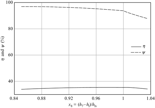
One of the features which is important for reheat cycle design is that there is an optimum pressure for the reheating process at which the efficiency of the cycle is maximized for any fixed boiling temperature. This optimum can be observed if the cycle efficiency is plotted against the pressure ratio across the HPT. Figure 5.10 illustrates the existence of the optimum pressure ratio for a relevant case study. Assume that the working fluid is steam and that the highest temperature of the working fluid is fixed to T₅ = T₇ = 400 °C. The variation of cycle efficiency with pressure ratio PR = P₅/P₆ is shown for five values of boiling temperature (see Figure 5.10). The optimum pressure ratio is in the range of 3 to 4.6. The vapor quality at the turbine exit decreases for optimum expansion from x₈ = 0.94 when T_b = 200 °C to x₈ = 0.83 and boiling temperature is 280 °C.

Example 5.3

This example considers a single-reheat ideal Rankine cycle with a configuration similar to that indicated in Figure 5.7. The condensation temperature is T_c = 30 °C, boiling is at 280 °C, and steam is superheated up to 400 °C. Determine the optimum pressure ratio for the HPT, the maximum cycle efficiency, and the mass-specific work for the HPT and LPT and show the T–s diagram of the cycle.

The mass and energy balances for each component of the cycle are written as indicated in Table 5.1. The mass flow rate is the same for all state points, hence the mass-specific quantities can be used. The pressure ratio over the HPT is varied in the range of 3 to 4 and a maximum efficiency of the cycle in the given conditions is determined to be 40.44% for PR_opt = 3.066. For this case the mass-specific work developed by the HPT is 280.1 kJ/kg, and the LPT develops 1099 kJ/kg. The cycle diagram is shown in Figure 5.11.

5.2.4 Ideal Regenerative Rankine Cycle

At the beginning of the twentieth century, the regenerative Rankine cycle started to be used for power generation with improved efficiency. This cycle is a modification of the basic Rankine cycle. It consists of applying internal regeneration within the cycle aimed at preheating the working fluid after the liquid pressurization process. Regeneration increases the average boiler temperature and makes the ideal Rankine cycle approach better than the Carnot cycle.

Let us compare the ideal Rankine cycle represented in Figure 5.1 with the Carnot cycle. As observed, the process path 3–4–1–2 resembles a part of the Carnot cycle. Also the boiling process 3a–3b is an isothermal heat input such as that in the Carnot cycle. However, compared to the Carnot processes, processes 2–3a and 3b–3 show large abatement because these are non-isothermal heat additions. In particular, process 2–3a has a negative effect on cycle efficiency because it dramatically reduces the temperature at which heat input occurs. The idea of regeneration consists of transferring heat internally from expansion process 3–4 to preheating process 2–3a such that the need for heat input at a lower temperature (below boiling) is reduced or eliminated.

The schematic of the ideal regenerative Rankine cycle is presented in Figure 5.12a. Imagine that the turbine is “surrounded” by a stream of working fluid in liquid phase which receives heat by heat transfer from the expanding flow to increase its temperature according to process 2–3. The rate of heat is indicated in the figure with ${\dot{\mathit{Q}}}_{\mathrm{ph}}$. Because there is a heat transfer process superimposed over the isentropic expansion process in the ideal regenerative Rankine cycle the turbine will operate non-adiabatically (and isentropically, that is with no irreversibilities due to expansion) according to a process represented by the line 5–7 in Figure 5.12b.

The energy balance equation for the regeneration process (see Figure 5.12) can be written with mass-specific quantities as shown below:

${\mathit{q}}_{\mathrm{ph}}+{\mathit{w}}_{\mathrm{t}}={\mathit{h}}_5-{\mathit{h}}_7\mathrm{a}\mathrm{n}\mathrm{d}{\mathit{q}}_{\mathrm{ph}}={\mathit{h}}_3-{\mathit{h}}_2$

One also imposes that the ideal regenerative Rankine cycle develops the same turbine work as the internally reversible Rankine cycle of basic configuration operating under the same condition (w_t = h₅ − h₆); hence one has:

${\mathit{h}}_3-{\mathit{h}}_2+{\mathit{h}}_5-{\mathit{h}}_6={\mathit{h}}_5-{\mathit{h}}_7\to {\mathit{h}}_6-{\mathit{h}}_7={\mathit{h}}_3-{\mathit{h}}_2$

The efficiency of the basic, internally reversible Rankine cycle operating under the same conditions as the ideal regenerative cycle (T_c, T_b, T₅ are the same) is expressed as follows:

$\mathit{\eta }=\frac{{\mathit{w}}_{\mathrm{t}}-{\mathit{w}}_{\mathrm{p}}}{{\mathit{q}}_{\mathrm{in}}}=\frac{{\mathit{h}}_5-{\mathit{h}}_6-\left({\mathit{h}}_2-{\mathit{h}}_1\right)}{{\mathit{h}}_5-{\mathit{h}}_2}=1-\frac{{\mathit{h}}_6-{\mathit{h}}_1}{{\mathit{h}}_5-{\mathit{h}}_2}$

The efficiency of the ideal regenerative Rankine cycle can be expressed as follows:

${\mathit{\eta }}_{\mathrm{R}}=\frac{{\mathit{w}}_{\mathrm{t}}-{\mathit{w}}_{\mathrm{p}}}{{\mathit{q}}_{\mathrm{in}}}=\frac{{\mathit{h}}_5-{\mathit{h}}_7-\left({\mathit{h}}_3-{\mathit{h}}_2\right)-\left({\mathit{h}}_2-{\mathit{h}}_1\right)}{{\mathit{h}}_5-{\mathit{h}}_3}=1-\frac{{\mathit{h}}_7-{\mathit{h}}_1}{{\mathit{h}}_5-{\mathit{h}}_3}$

Comparing η and η_R expressed with the help of above three equations, one has that

${\mathit{\eta }}_{\mathrm{R}}=1-\frac{{\mathit{h}}_6-{\mathit{h}}_1}{{\mathit{h}}_5-{\mathit{h}}_3}+\frac{{\mathit{h}}_3-{\mathit{h}}_2}{{\mathit{h}}_5-{\mathit{h}}_3}>1-\frac{{\mathit{h}}_6-{\mathit{h}}_1}{{\mathit{h}}_5-{\mathit{h}}_2}+\frac{{\mathit{h}}_3-{\mathit{h}}_2}{{\mathit{h}}_5-{\mathit{h}}_3}>\mathit{\eta }$

where one notices that h₅ − h₂ > h₅ − h₃ > 0 (see Figure 5.12). Thus, it is demonstrated that the efficiency of the ideal regenerative Rankine cycle is necessarily higher than that of the ideal Rankine cycle of basic configuration operating between the same temperature limits. This increase in efficiency can be as much as 18–20% when the working fluid is steam and the boiling temperature in the range of 200–300 °C.

According to Figure 5.12a, the regenerative Rankine cycle cannot be implemented in practice because it is not convenient to extract heat from an expanding flow; the turbine construction would be too complicated and not feasible. In addition, due to heat extraction, the moisture at the turbine outlet is far too high (it can reach more than 60%).

What can be done to overcome these construction obstacles is to extract some steam from the turbine at intermediate pressures and condense it to further extract heat for water preheating. This process will diminish turbine work but it will increase the cycle efficiency because the average temperature at source side becomes higher. There are several known ways to transfer heat from the condensing steam extracted from the turbine to the water preheating process. The simplest system is the use of a closed feedwater heater that represents, in fact, a condenser.

In Figure 5.13 is presented a regenerative Rankine cycle with a closed feedwater heater. After it condenses in the regenerator (process 7–8), the working fluid is throttled to lower pressure using a device called a “steam trap” (process 8–9). A fraction f of vapor is extracted from the turbine at intermediate pressure (in state 7) and directed toward the regenerator. The remaining vapor (that is the fraction 1 − f ) is expanded up to condenser pressure (state 10). In a first section of the condenser (10–11) the steam reduces the vapor quality to an intermediate value that corresponds to state 11. The vapor quality of the throttled working fluid in 9 is the same as that in state 11, hence x₉ = x₁₁ = x₁₂. The condensation process continues with full flow until saturated liquid is obtained in 1. The relevant mass balance equations and the extracted vapor fraction (f ∈ [0, 1]) for the system are:

${\dot{\mathit{m}}}_6={\dot{\mathit{m}}}_7+{\dot{\mathit{m}}}_{10};\mathit{f}{\dot{\mathit{m}}}_6={\dot{\mathit{m}}}_7;{\dot{\mathit{m}}}_9+{\dot{\mathit{m}}}_{11}={\dot{\mathit{m}}}_{12}$

The energy balance of the regenerator also imposes that

$\left(1-\mathit{f}\right)\left({\mathit{h}}_7-{\mathit{h}}_8\right)={\mathit{h}}_3-{\mathit{h}}_2$

The exergy balance of the regenerator will determine the irreversibility due to heat transfer, owing to the fact that T₇ = T₈ > T₃ > T₂. The exergy balance is as follows:

$\mathit{e}{\mathit{x}}_2+\mathit{f}\mathit{e}{\mathit{x}}_7=\mathit{e}{\mathit{x}}_3+\mathit{f}\mathit{e}{\mathit{x}}_8+\mathit{e}{\mathit{x}}_{\mathrm{d},\mathrm{reg}}$

where ex_d is the exergy destroyed by the regenerator. In addition, there is exergy destruction due to throttling process 8–9. The exergy balance for the steam trap can be written as follows to determine the exergy destruction:

$\mathit{f}\mathit{e}{\mathit{x}}_8=\mathit{f}\mathit{e}{\mathit{x}}_9+\mathit{e}{\mathit{x}}_{\mathrm{d},\mathrm{trap}}$

The energy balance on the condenser requires

$\mathit{f}{\mathit{h}}_9+\left(1-\mathit{f}\right){\mathit{h}}_{10}={\mathit{h}}_1+{\mathit{q}}_{\mathrm{c}}$

where q_c represents the mass-specific heat flux rejected by the condenser (in kJ/kg). If $\dot{\mathit{m}}$ is the mass flow rate of working fluid in state 1, then, with reference to Figure 5.13, it results that the heat rate rejected by the condenser is

${\dot{\mathit{Q}}}_{\mathrm{c}}=\dot{\mathit{m}}{\mathit{q}}_{\mathrm{c}}={\dot{\mathit{Q}}}_{\mathrm{c}1}+{\dot{\mathit{Q}}}_{\mathrm{c}2}=\dot{\mathit{m}}({\mathit{q}}_{\mathrm{c}1}+{\mathit{q}}_{\mathrm{c}2})$

where q_c1 = (1 − f)(h₁₀ − h₁₁) and q_c2 = h₁₂ − h₁, and one also notes that h₉ = h₁₁ = h₁₂.

The vapor quality of the extracted steam in regenerative Rankine schemes is slightly below unity. The efficiency of the regenerative cycle is slightly influenced by the quality of extracted steam. For higher quality, the energy efficiency tends to be better, whereas the exergy efficiency is not influenced. This evolution can be observed in Figure 5.14, which indicates that the best extraction is obtained when vapor quality is around 0.9. It also results that it is detrimental to extract superheated steam because both the energy and exergy efficiencies decrease sharply.

The exergy destructions within the cycle can be reduced and the energy efficiency can be improved if the steam trap is replaced with a pump followed by a mixer. Such a scheme is denoted as a regenerative Rankine cycle with a closed feedwater heater and pump and is represented in Figure 5.15. The system has the advantage of reducing the size of the condenser, and it also reduces the pumping power. However, there are still exergy destructions related to the regenerator and the mixer (the mixer is in fact a direct contact heat exchanger, which, in this case, mixes streams that have about the same temperature). The energy balance on the regenerator becomes in this case:

$\left(1-\mathit{f}\right){\mathit{h}}_2+\mathit{f}{\mathit{h}}_8=\left(1-\mathit{f}\right){\mathit{h}}_3+\mathit{f}{\mathit{h}}_9$

whereas the exergy balance becomes

$\left(1-\mathit{f}\right)\mathit{e}{\mathit{x}}_2+\mathit{f}\mathit{e}{\mathit{x}}_8=\left(1-\mathit{f}\right)\mathit{e}{\mathit{x}}_3+\mathit{f}\mathit{e}{\mathit{x}}_9+\mathit{e}{\mathit{x}}_{\mathrm{d},\mathrm{reg}}$

The energy and exergy balances for the mixer are written as

$\left(1-\mathit{f}\right){\mathit{h}}_3+\mathit{f}{\mathit{h}}_{10}={\mathit{h}}_4\mathrm{a}\mathrm{n}\mathrm{d}\left(1-\mathit{f}\right)\mathit{e}{\mathit{x}}_3+\mathit{f}\mathit{e}{\mathit{x}}_{10}=\mathit{e}{\mathit{x}}_4+\mathit{e}{\mathit{x}}_{\mathrm{d},\mathrm{mix}}$

For the ideal cycle exemplified in Figure 5.16 the exergy destruction at the regenerator is 22.86 kJ/kg while the exergy destruction at the mixer is negligible (0.046 kJ/kg). The extracted steam fraction is 11.3% and the energy efficiency of the cycle is slightly improved with respect to the energy efficiency of the one with the steam trap analyzed previously: 35.4% versus 35.1%. This cycle is also illustrated in the P–h diagram in Figure 5.17 where the non-isobaric processes are made apparent.

The exergy destruction in the regenerator–mixer system can be further reduced if the closed feedwater heater is replaced with an open feedwater heater (OFW). This is in fact a direct contact heat exchanger. An improved Rankine plant design of regenerative type is introduced in Figure 5.18. The exergy destruction in the OFW must be smaller with respect to the closed feedwater heater because the temperature of extracted steam can be equal to the temperature of the condensate. In addition, the OFW has a simpler and cheaper construction than the closed one. An example of an ideal cycle with this configuration is illustrated in Figure 5.19.

A combination of open and closed feedwater heaters with multiple steam extraction pressures can be used to increase cycle efficiency even more. This approach is used in practice as a technical and economical trade-off for steam Rankine power stations. The OFW is cheaper and more efficient than the closed feedwater heater, but requires additional pumps, which involve more costs. On the contrary, the closed feedwater heaters are more costly and less efficient, but these heaters do not necessitate additional pumps. Moreover, multiple feedwater heaters of closed type can be cascaded using steam traps and a single pump, although this solution destroys more exergy.

Example 5.4

Let us consider a regenerative steam Rankine cycle of the configuration illustrated in Figure 5.13. Assume that T_c = 30 °C, T_b = 200 °C, ΔT_sh = 200 °C and that all internal processes are reversible except the feedwater heater, which operates with a temperature difference for heat transfer defined by ΔT_reg = T₇ − T₃ = 10 °C (see Figure 5.13 for the state point numbers). We want to determine the extracted steam ratio and the energy and exergy efficiencies and to represent the cycle in the T–s diagram.

In order to solve this problem mass, energy, entropy, and exergy balance equations must be written for each system component; hence for the nine components of the system, there will be in total 27 equations. Three equations come from the fact that the pump and the turbines operate isentropically, which means that s₂ = s₁; s₆ = s₇ = s₁₀. In addition, the extracted steam fraction is defined by Equation (5.8), and because all internal processes are reversible the mechanical and electrical efficiency are η_m = η_el = 1. In total one has 33 equations that form a closed system that can be solved to determine thermodynamic parameters at all of the state points.

A simple code can be written to solve the algebraic system numerically. Here we give the solution obtained with EES as shown in Table 5.9, where the thermodynamic parameters for each of the state points is given. For the specific exergy calculation a reference state must be assumed. As in previous examples, the reference state for the steam Rankine cycle is taken to be liquid water at the standard T₀, P₀. Once the thermodynamic states are determined, the extracted steam fraction results directly from Equation (5.8), which gives the solution f = 12.7%. The energy efficiency is 35.1%. To calculate the exergy efficiency, one assumes that the heat source is at a constant temperature level equal to the temperature of the thermodynamic state at the turbine inlet, T_so = T₆ = T_b + ΔT_sh = 673 K. Therefore the Carnot factor is 0.5571 and the exergy efficiency is 63.06%. The cycle diagram is presented at scale in Figure 5.20.

Table 5.9

State Point Parameters Calculated for Example 5.4

State	P (kPa)	T (K)	v (m3/kg)	x	h (kJ/kg)	s (kJ/kgK)	ex (kJ/kg)
1	4.246	303.2	0.001004	0	125.7	0.4365	0.1745
2	1554	303.2	0.001004	-0.3738	127.2	0.4365	1.73
3	1554	371.2	0.001041	-0.2271	411.8	1.283	33.84
4	1554	473.2	0.001156	0	852.4	2.331	162.1
5	1554	473.2	0.1273	1	2793	6.431	879.7
6	1554	673.2	0.1958	1.238	3255	7.252	1097
7	134	381.2	1.287	0.9984	2685	7.252	527.3
8	134	381.2	0.00105	0	453	1.397	41.2
9	4.246	303.2	4.432	0.1347	453	1.516	5.573
10	4.246	303.2	27.97	0.8503	2192	7.252	34.25
11	4.246	303.2	4.432	0.1347	453	1.516	5.573
12	4.246	303.2	4.432	0.1347	453	1.516	5.573

Example 5.5

In Figure 5.21 is exemplified a steam Rankine power plant with multiple feedwater heaters and steam extraction points. The cycle operates according to the following main parameters: T_c = 30 °C, T_b = 200 °C, ΔT_sh = 200 °C.

Mass balance equations for this system become significantly more complex with respect to the other systems discussed previously. Table 5.10 gives the mass balance equations for all components of the system and also introduces the steam extraction fractions f_i, i = 11, 14, 17, 18. Using the steam fractions the energy and exergy balances can be written for each plant component according to Equations (5.8)–(5.14).

Table 5.10

Mass Balance Equations for Rankine Cycle Represented in Figure 5.21

Component	MBE	Component	MBE	f definitions
LPP	${\dot{\mathit{m}}}_2={\dot{\mathit{m}}}_1$	CFWH2–3	${\dot{\mathit{m}}}_3={\dot{\mathit{m}}}_2;{\dot{\mathit{m}}}_{18}={\dot{\mathit{m}}}_{19}={\dot{\mathit{m}}}_{20}$	${\dot{\mathit{m}}}_{11}={\mathit{f}}_{11}{\dot{\mathit{m}}}_{10}$
HPP	${\dot{\mathit{m}}}_5={\dot{\mathit{m}}}_4$	OFWH	${\dot{\mathit{m}}}_3+{\dot{\mathit{m}}}_{16}+{\dot{\mathit{m}}}_{17}={\dot{\mathit{m}}}_4$	${\dot{\mathit{m}}}_{14}={\mathit{f}}_{14}{\dot{\mathit{m}}}_{10}$
ST15–16	${\dot{\mathit{m}}}_{16}={\dot{\mathit{m}}}_{15}$	CFWH5–6	${\dot{\mathit{m}}}_6={\dot{\mathit{m}}}_5;{\dot{\mathit{m}}}_{13}+{\dot{\mathit{m}}}_{14}={\dot{\mathit{m}}}_{15}$	${\dot{\mathit{m}}}_{17}={\mathit{f}}_{17}{\dot{\mathit{m}}}_{10}$
PH	${\dot{\mathit{m}}}_8={\dot{\mathit{m}}}_7$	CFWH6–7	${\dot{\mathit{m}}}_7={\dot{\mathit{m}}}_6;{\dot{\mathit{m}}}_{11}={\dot{\mathit{m}}}_{12}$	${\dot{\mathit{m}}}_{18}={\mathit{f}}_{18}{\dot{\mathit{m}}}_{10}$
B	${\dot{\mathit{m}}}_9={\dot{\mathit{m}}}_8$	STB	f11 + f14 + f17 + + f18 + f21 = 1	${\dot{\mathit{m}}}_{21}={\mathit{f}}_{21}{\dot{\mathit{m}}}_{10}$
SH	${\dot{\mathit{m}}}_{10}={\dot{\mathit{m}}}_9$	COND	${\dot{\mathit{m}}}_{20}+{\dot{\mathit{m}}}_{21}={\dot{\mathit{m}}}_1$	${\dot{\mathit{m}}}_1=\left({\mathit{f}}_{18}+{\mathit{f}}_{21}\right){\dot{\mathit{m}}}_{10}$

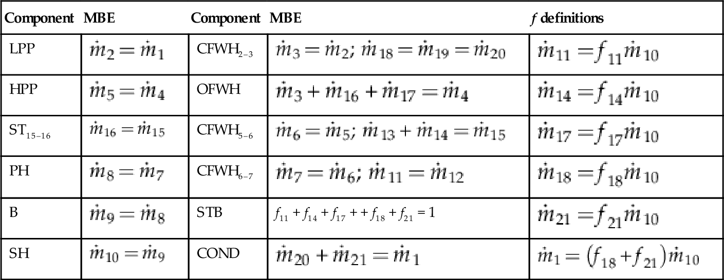
MBE, Mass balance equation; LPP, low-pressure pump; CFWH, closed feedwater heater; OFWH, open feedwater heater; HPP, high-pressure pump; ST, steam trap; PH, preheater; B, boiler; SH, superheater; STB, steam turbine; f, steam extraction fraction.

Optimal flow extraction fractions can be determined based on various multivariable optimization methods to maximize the energy efficiency of the cycle. Here the genetic algorithm optimization implemented in EES is used to maximize cycle efficiency; the optimum extraction fractions are determined as follows: f₁₁ = 5.4%, f₁₄ = 4.7%, f₁₇ = 5.8%, f₁₈ = 3.8%. The maximized energy efficiency for the ideal Rankine cycle case study is η = 36.5%. The exergy efficiency of the cycle is 65.5%; exergy is destroyed in feedwater heaters, steam traps, the condenser, and the steam generator. The thermodynamic cycle is represented in the T–s diagram shown in Figure 5.22.