7.3 Wind Energy Systems

Wind energy is a significant renewable energy resource which has shown rapid growth in recent years. The cost of wind energy has achieved reasonable values such that wind energy farms are now constructed in many locations around the world. Germany, Denmark, and Spain are the lead countries in installing wind energy capacities. Wind energy can be regarded as a meteorological variable signifying the energy content of the wind.

The important parameter for meteorological modeling of wind is the wind velocity. In meteorology an atmospheric boundary is considered for predicting the local or regional winds by simulation. Other meteorological variables such as temperature, pressure, and humidity of the atmosphere are also important in wind occurrence. Such information together with measured velocity data are necessary for determining locations to install wind energy farms, estimating their capacity and efficiency.

Wind is in fact a form of mechanical energy. It has to be harvested by appropriately engineered devices and converted into other useful energies like electric energy. The major technical problem of a wind energy conversion system is represented by the fluctuating and intermittent nature of the wind. The harvesting system (typically a wind turbine) must react fast to the presence of wind or change in its direction and intensity. It is important to be able to store the mechanical energy harvested from wind. Several systems of wind energy storage are possible, where the mechanical energy resulting from wind is stored in various forms: kinetic (flywheels), electrochemical (batteries), chemical (hydrogen), thermomechanical (compressed air), etc. Nevertheless, the most used systems are electrical generators actuated by wind energy, having local storage capacities in batteries, and possibly being equipped with grid connecting systems. Wind turbine efficiency reaches around 35–50% with the current technology.

The harvested wind energy is normally converted into shaft rotation by a wind turbine. The mechanical energy can then be used directly. For smooth generation, the mechanical energy can be stored in some devices able to retrieve it in mechanical form, such as flywheels, hydro-storage, or compressed air. A typical direct use of wind energy is water pumping; others include grain milling, wood cutting, etc. The shaft rotating mechanical energy can be converted by appropriate electric generators into electrical energy. Common types of wind turbines are illustrated in Figure 7.40.

The most important wind turbine for power generation is the HAWT (horizontal axis wind turbine). The electrical energy generated by wind can be stored locally or transmitted to the grid or further used for hydrogen generation through water photosynthesis. Furthermore, hydrogen can be converted to ammonia though the well-matured Haber–Bosh process; this process requires additional consumption of electricity.

For thermodynamic analysis a fictitious boundary can be drawn around the turbine to delimit a control volume, as indicated in Figure 7.41. Outside this boundary, there is no significant modification of the velocity of air. On the contrary, inside the control volume the air feels the presence of the turbine; thus it accelerates or decelerates according to the laws of energy conservation and applicable constraints. Basically, the upstream area of the control volume (A₁) is much smaller than the downstream area (A₂). Thus the velocity upstream (V₁) is much higher than the velocity downstream (V₂).

The geometry of the control volume is similar to that of a nozzle which extracts the work W from the wind. The average velocity of the wind is denoted with $\overline{\mathit{V}}=\left({\mathit{V}}_1+{\mathit{V}}_2\right)/2$, and the mass flow rate of air is approximated with $\dot{\mathit{m}}=\mathit{\rho }\mathit{A}\overline{\mathit{V}}$. Thus the rate of variation of wind momentum is $\dot{\mathit{m}}\left({\mathit{V}}_2-{\mathit{V}}_1\right)=\mathit{\rho }\mathit{A}\overline{\mathit{V}}\left({\mathit{V}}_2-{\mathit{V}}_1\right)$. According to the second law of dynamics, the force exerted on the rotor is $\mathit{F}=-\mathit{\rho }\mathit{A}\overline{\mathit{V}}\left({\mathit{V}}_2-{\mathit{V}}_1\right)$. Based on the force and the average velocity it results that the work extracted by the rotor is $\mathit{W}=\mathit{\rho }\mathit{A}\overline{\mathit{V}}\left({\mathit{V}}_2-{\mathit{V}}_1\right)\times \overline{\mathit{V}}$. This work can be also calculated based on the kinetic energy variation of the air, that is $\mathit{W}=0.5\mathit{\rho }\mathit{A}\overline{\mathit{V}}\left({\mathit{V}}_1^2-{\mathit{V}}_2^2\right)$. The equality of the two expressions for W results in $\overline{\mathit{V}}=\left({\mathit{V}}_1+{\mathit{V}}_2\right)/2$ which in fact justifies the definition of the average velocity as the arithmetic mean. Using the notation α = V₂/V₁, one obtains simply that the work extraction is

$\mathit{W}=\mathit{\rho }\frac{\mathit{A}{\mathit{V}}_1^3}{4}\left[\left(1+\mathit{\alpha }\right)\left(1-{\mathit{\alpha }}^2\right)\right]$

The quantities ρ, A and V₁ should be assumed constant for the analysis; thus for a given wind velocity, outside temperature, and pressure (which fixes the air density) and a given wind turbine area, the generated work is a function of velocities ratio only, W = W(α). It is simple to show that the maximum of the work is obtained at α = 1/3, which corresponds to

${\mathit{W}}_{\text{max}}=\frac{8}{27}\mathit{\rho }\frac{\mathit{A}{\mathit{V}}_1^3}{4}$

The efficiency of mechanical work production from wind energy must be equal to the useful shaft work generated divided to the wind energy, both given per unit of turbine surface area. The wind energy is the kinetic energy (0.5ρAV₁³). Thus the theoretical maximum energy efficiency of the wind energy conversion is

${\mathit{\eta }}_{\text{max}}=\raisebox{1ex}{$\frac{8}{27}\mathit{\rho }\frac{\mathit{A}{\mathit{V}}_1^3}{4}$}\!\left/ \!\raisebox{-1ex}{$\frac{1}{2}\mathit{\rho A}{\mathit{V}}_1^3$}\right.=\frac{16}{27}=59.3\mathit{\%}$

.

Looking back to the equation giving the work extracted by the rotor, W, the quantity between square brackets defines the power coefficient of the rotor efficiency given by

${\mathit{C}}_{\mathrm{P}}=\left[\left(1+\mathit{\alpha }\right)\left(1-{\mathit{\alpha }}^2\right)\right]/2.$

The turbine efficiency becomes

$\mathit{\eta }={\mathit{C}}_{\mathit{P}}$

As given above, the maximum value of C_P,max is 0.593; however, the efficiency found in practice is in the range 35%–45%. With Equation (7.26) the work extraction reduces to

$\mathit{W}=\mathit{\rho }{\mathit{C}}_{\mathit{P}}\frac{\mathit{A}{\mathit{V}}_1^3}{2}.$

Note also that during a period of time (e.g., day, month, season) the wind velocity (V₁) varies. Another aspect regarding wind energy conversion relates to the variation of the wind speed at a certain location, during a year. The annual distribution probability of the wind velocity influences the total energy generated at a specific location during a year.

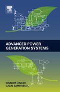
Weibull probability distribution can be used to model the occurrence of wind velocity based on two parameters k and c, according to h(V) = k/c(V/c)^k − 1 exp[−(V/c)^k]; for parameter k = 2 this probability distribution function is called the Rayleigh distribution

$\mathit{h}\left(\mathit{V}\right)=\frac{2\mathit{V}}{{\mathit{c}}^2}exp\left[-{\left(\frac{\mathit{V}}{\mathit{c}}\right)}^2\right].$

The Rayleigh distribution for annual variation of wind velocity is exemplified in the plot in Figure 7.42 for the case c = 7 m/s; in the plot, the annual probability of occurrence of wind velocity is correlated with the cube of velocity. Two vertical lines are shown at cut-in speed (V_ci) assumed at 3 m/s and cut-out speed (V_co) assumed at 20 m/s. Outside the region delimited by V_ci and V_co the wind turbine does not operate. The hatched area on the plot, which corresponds with the wind turbine operation domain, can be calculated with the integral

$\underset{{\mathit{V}}_{\mathrm{ci}}}{\overset{{\mathit{V}}_{\mathrm{co}}}{\int }}\mathit{h}\left(\mathit{V}\right)\mathit{d}\left({\mathit{V}}^3\right)=100\mathit{\%}\times {\mathit{V}}_{\mathrm{RMC}}^3$

where V_RMC one denotes the root mean cube wind velocity.

The gray area defines the root mean cube wind velocity as an average velocity that has 100% occurrence and generates the same amount of wind energy as the probable velocity profile described by the adopted probability distribution function. Thus the generated mechanical energy by the turbine operating at a constant rate throughout the year can be written as

$\mathit{W}=\frac{1}{2}\mathit{\rho }{\mathit{C}}_{\mathrm{p}}\mathit{A}{\mathit{V}}_{\mathrm{RMC}}^3$

where

${\mathit{V}}_{\mathrm{RMC}}^3={\int }_{{\mathit{V}}_{\mathrm{ci}}}^{{\mathit{V}}_{\mathrm{co}}}\mathit{h}\left(\mathit{V}\right)\mathit{d}\left({\mathit{V}}^3\right)$

When a wind turbine location is selected, it is important to know the average wind velocity in that location, because the turbine energy efficiency is specified by the manufacturer at a rated value which corresponds to a rated wind velocity (V_r). If the wind velocity is different than the turbine rating value, then a capacity factor can be used (as indicated by the manufacturer) to determine the generated power under the actual conditions. The capacity factor is defined as the percentage of the nominal power that the wind turbine generates in actual wind conditions. In this case the energy efficiency of the wind turbine becomes

$\mathit{\eta }\left(\mathit{V}\right)={\mathit{C}}_{\mathrm{f}}\left(\mathit{V}\right)$

where C_f(V) is the capacity factor expressed as a function of the actual wind velocity. The capacity factor is small at low and high velocities and typically has a maximum value at the design point.

Figure 7.43 exemplifies a typical variation of the wind capacity factor; on the same plot is superimposed an assumed annual occurrence of wind speed. It is possible to calculate the average wind velocity based on velocity occurrence; in this case, the average velocity is defined as the velocity which occurs at 100%; in other words, when the area between the h(V) × V curve is equal with the grey area shown in the figure. Therefore:

$\overline{\mathit{V}}=\underset{{\mathit{V}}_{\mathrm{ci}}}{\overset{{\mathit{V}}_{\mathrm{co}}}{\int }}\mathit{h}\left(\mathit{V}\right)\mathit{V}\mathrm{d}\mathit{V}$

For the numerical example shown in the figure, the average wind velocity result is $\overline{\mathit{V}}=5.87\mathrm{m}/\mathrm{s}$ which gives an average capacity factor of C_f = 45.7%. In general one can write the average turbine efficiency as given by

$\overline{\mathit{\eta }}={\mathit{C}}_{\mathrm{f}}\left(\overline{\mathit{V}}\right)$

The average power generation of a wind turbine placed in certain location becomes

$\overline{\mathit{W}}=\frac{1}{2}\mathit{\rho }\mathit{A}{\mathit{C}}_{\mathrm{f}}\left(\overline{\mathit{V}}\right){\mathit{V}}_{\mathrm{RMC}}^3$

Another effect, the wind chill, can influence in some measure the efficiency of wind turbine generators. Faster cold wind makes the air feel colder than when wind is not present because it removes heat from our bodies faster due to intensified heat transfer by convection. Wind chill is a measure of this effect and is defined as the hypothetical air temperature in calm conditions (air speed, V = 0) that would cause the same heat flux from the skin as occurs at the actual air speed and temperature. Wind chill temperature can be estimated with

${\mathit{T}}_{\mathrm{wch}}=21.68+1.12{\mathit{T}}_0-38.58{\mathit{V}}^{0.16}+\left(0.83{\mathit{T}}_0+14.76\right){\mathit{V}}^{0.16}$

where T is temperature in °C, indices “wch” and “a” denote wind chill and surroundings air, and V is the wind speed in km/h.

Thus, a rigorous application of Equation (7.34) implies the estimation of the air density at wind chill temperature. The air density depends on the atmospheric pressure and temperature (a simple calculation of the air density can be based on the ideal gas law, ρ = ρ_ref × T_ref/T₀ × P₀/P_ref where the index 0 represents the actual environment, ref is reference environment, and T is temperature in K and P is pressure). Due to expansion, air suffers additional cooling between upstream (1) and downstream states (2). Thus the average air density is $\overline{\mathit{\rho }}=\left({\mathit{\rho }}_1+{\mathit{\rho }}_2\right)/2$, where ρ_1,2 are calculated with (T_1,2, P_1,2) and T_1,2 are wind chill temperatures calculated with Equation (7.35). Thus a more accurate energy efficiency expression, accounting for wind chill temperature, is

$\overline{\mathit{\eta }}={\mathit{C}}_{\mathrm{f}}\left(\overline{\mathit{V}}\right)\overline{\mathit{\rho }}/{\mathit{\rho }}_0$

where the index 0 indicates the temperature of the surroundings. The energy conversion of wind energy can be up to 2% higher than the turbine capacity factor.

The exergy efficiency of a wind turbine is defined as the work produced per exergy associated with the wind. The work generated by the turbine can be calculated, as discussed above, with $\mathit{W}=0.5{\mathit{C}}_{\mathrm{f}}\left(\overline{\mathit{V}}\right)\overline{\mathit{\rho }}\mathit{A}{\mathit{V}}_{\mathrm{RMC}}^3$. The exergy associated with the wind surrounding the turbine must comprise the kinetic energy of the wind (which is a form of exergy) and the thermomechanical exergy of the wind. The thermomechanical exergy of the wind must be calculated with respect to wind chill temperature, because this is the temperature of the medium in the vicinity of the turbine. The wind has a higher exergy upstream (Ex₁) than downstream (Ex₂). Thus the exergy that enters the system is the difference (Ex = Ex₁ − Ex₂). Using appropriate expressions for thermomechanical and kinetic energy it results that

$\mathit{E}\mathit{x}=\mathit{W}+\overline{\mathit{\rho }}\mathit{A}\overline{\mathit{V}}\times \left\{{\overline{\mathit{C}}}_{\mathrm{p}}\left({\mathit{T}}_1-{\mathit{T}}_2\right)-{\mathit{T}}_0\left[{\overline{\mathit{C}}}_{\mathrm{p}}ln\left(\frac{{\mathit{T}}_2}{{\mathit{T}}_1}\right)-\mathit{R}ln\left(\frac{{\mathit{P}}_2}{{\mathit{P}}_1}\right)-{\overline{\mathit{C}}}_{\mathrm{p}}\left(1-\frac{\overline{\mathit{T}}}{{\mathit{T}}_0}\right)\right]\right\}$

where $\overline{\mathit{\rho }}\mathit{A}\overline{\mathit{V}}$ is the mass flow rate of air, T_1,2 are the wind chill temperatures upstream and downstream of the turbine, T₀ is the temperature of the surroundings, $\overline{\mathit{T}}$ is the arithmetic mean of temperatures T_1,2, pressures P_1,2 are upstream and downstream, respectively, ${\overline{\mathit{C}}}_{\mathrm{p}}$ is the specific heat, and R is the ideal gas constant. The first term in braces represents the enthalpy difference, the second term is the entropy difference, and the irreversibility due to heat transfer between the stream of air and the surroundings; basically, the expression in braces is the specific thermomechanical exergy consumed by the system. The exergy efficiency becomes

$\mathit{\psi }=\frac{\mathit{W}}{\mathit{Ex}}$

Two basic categories of wind turbine design do exist, namely the horizontal axis wind turbine (HAWT) and the vertical axis wind turbines (VAWT). The horizontal axis wind turbines have emerged as the dominant technology. They have the rotor axis horizontal and in line with the wind direction. The common designs have the generator and the blade fixed on a rotating structure in the top of a tower. The mechanical system also comprises a gear box that multiplies the rotation of the blades. Compared to the VAWT, the HAWT achieves higher efficiency. The VAWT operates well in fluctuating wind amplitude provided that its direction remains quasi-constant.

One important feature of the VAWT is that it does not need to be pointed in the direction of the wind. Thus VAWT installation is appropriate where wind changes its direction very frequently. Another feature of the VAWT is that it allows placement of the generator and gear box in the lower side, closing the support system of the turbine.

The HAWT construction can differ in number of blades (generally two or three blades are used). The HAWT use airfoils to generate lift under the wind action and rotate the propeller. The operation of some VAWT designs is also based on the aerodynamic lift principle, but there are designs that use form drag and aerodynamic friction for operation. Drag-type turbines are designed such that the form drag generates a torque; a typical drag turbine is the Savonius, much used in rural areas. The operating principle of the Savonius wind turbine is illustrated schematically in Figure 7.44. The generated torque is due to the difference in pressure between the concave and convex surfaces of the blades and reaction forces of the deflected wind coming from behind the convex surface. The efficiency of the Savonius turbine is over 30%.

A more elaborate design of the VAWT, namely the Zephyr, is also presented in Figure 7.33. Itis designed to perform well in low wind speed and high turbulence conditions. For this reason, several Zephyr wind turbines can be installed close to each other to form a compact wind farm. The power coefficient of the Zephyr wind turbine is rather low (0.11) but the turbine has a good utilization factor, low cut-in speed, and high cut-off speed which make it competitive in urban areas.

Common models of lifting VAWT turbines are the triangular (delta) Darrieus turbine, the Giromill turbine, and the Darrieus–Troposkien turbine. The triangular Darrieus turbine has straight-blade geometry. The Giromill turbine is a low-load system with straight, vertical blades and an adjustable angle of attack to fit the best working conditions. The Darrieus–Troposkien turbine is the turbine most used for electric power generation. The blades of this turbines are airfoils assuming a Troposkien shape (which is a name derived from Greek meaning “the shape of a spinning rope”). Basically, the airfoil is a flexible blade connected to a vertical axis at two points (lower and upper);while rotating it approximates by revolution the shape of an ellipsoid. The blades can be made from light materials like aluminum, fiberglass, steel, or wood.

Apart from the wind turbine itself, wind power plants comprise several other important subsystems, such as yaw control, a speed multiplier (gear box), voltage–frequency and rotation controllers, voltage-raising and -lowering transformers (with the role of matching the generation, transmission, and distribution voltages at normal consumption levels), protection systems for over-current, over-speed, overvoltage, and atmospheric outbreaks, and other anomalous forms of operation. All these subsystems are sustained by a robust mechanical structure.

Figure 7.45 illustrates the simplified electric diagram of a wind power generation unit, including the main components and their functions. The system is equipped with general protection circuits, breakers, and over-current and reverse current protection. When a wind power generator is connected to the grid it is possible that—during low wind periods—the generated voltage is lower than the grid voltage. If this situation occurs the protection systems (see the figure) temporarily disconnect the system from the grid. Also if there is an over-current caused by a load too large, the thermal protection will disconnect the generator. The capacitors are used to correct the power factor of the generator and allow a soft start. The capacitors work together with a thyristor unit to soften the starting process of the generator. A small transformer is used to supply the auxiliary equipment. The system has a main transformer that allows connection of the unit to the grid. Local energy storage can be applied in batteries, in which case the system will include an inverter. Moreover, it is possible to couple several turbines to the main transformer, when it applies, rather than equipping each turbine with its own grid connection transformer.

The electrical system and electrical infrastructure of a wind power plant may account for 13–15% of the total installation costs. A breakdown of various costs for installing a 10-MW wind power unit is given in Figure 7.46. The electrical infrastructure is costly because it involves, among other things, massive work for grounding and lighting protection. The damage produced by lighting to wind farms and individual units is considerable. In Germany statistics show that lighting produces damage annually to 8% of installed wind turbines, while in Sweden this is 6% and in Denmark 4%.

The noise generated by wind power plants is also of major concern. The blades, the gearbox, the generator, the generator hub, the tower, and the auxiliary system all generate a significant amount of noise during operation. The noise of a wind power plant operating at 350 m far can be 10% higher than typical rural night background noise.

Considerable efforts have been deployed in recent years to develop techniques for reducing noise from wind turbines by proper design and installation. With current technology, the noise level of the main power plant components ranges from 40 to 98 dB(A). Nevertheless, protection against noise increases the capital cost of the power plant significantly. By the year 2004, the investment cost was around 50¢ per installed watt and 6¢ per generated kWh.

By expanding wind power generation capacities in recent years, the cost of installed kW and the cost of generated kWh has reduced significantly. The investment cost is presently about 30% higher than that for natural gas power plants, while the generation cost is about 3.5¢/kWh.

7.4 Geothermal Power Generation Systems

Geothermal energy is a form of thermal energy that is available on some regions of the earth’s surface at temperature levels in the range of about 35–500 °C, even though most geothermal locations provide temperature levels up to 250 °C. Geothermal heat is used either for process heating or is converted into electricity through appropriate heat engines. A large palette of heat-consuming processes can be supplied by geothermal energy, including space and water heating applications, industrial processes, various supply procedures in agriculture and food industry, etc. Figure 7.47 illustrates the global utilization of geothermal heat.

It can be observed from the graph that most of the geothermal applications are ground source heat pump systems. In recent years there has been substantial development in geothermal energy, with major interest in the ground source heat pump, hydrogen production from geothermal energy, and installing electrical plants supplied by geothermal heat. Some historical facts regarding geothermal development in Canada are indicated in Table 7.12.

As a source of heat, the limit of geothermal energy conversion is governed by the Carnot factor. Thus, it is important to assess the range of the Carnot factor for geothermal reservoirs. Additionally, it is useful to analyze relevant irreversibilities specific to geothermal energy conversion. Thus one can obtain a general picture of the thermodynamic limits of geothermal energy conversion into work.

We will analyze, as a first step, the temperature level of geothermal sources and the nature of geothermal fluid. The average increase in temperature with depth—called the geothermal gradient—is about 0.03 °C/m, or 30 °C/km for a few kilometers near the earth’s surface. Values as low as about 10 °C/km are found in ancient continental crust and very high values (> 100 °C/km) are found in areas of active volcanism.

Heat from the earth’s depths is transported to the surface in three possible ways, characterized by the type of geothermal field: hot water, wet steam, and dry steam. Hot water fields contain reservoirs of water with temperatures between 60 and 100 °C, and are most suitable for space heating and agricultural applications. For hot water fields to be commercially viable, they must contain a large amount of water with a temperature of at least 60 °C and lie within 2000 m of the surface. Wet steam fields contain water under pressure and usually measure 100 °C.

These are the most common commercially exploitable fields. When the water is brought to the surface, some of the water flashes into steam, and the steam may drive turbines that can produce electrical power. Dry steam fields are geologically similar to wet steam fields, except that superheated steam is extracted from the aquifer. Dry steam fields are relatively uncommon. Because superheated water explosively transforms into steam when exposed to the atmosphere, it is much safer and generally more economical to use geothermal energy to generate electricity, which is much more easily transported.

$\mathit{e}\mathit{x}=\mathit{h}\left(\mathit{T},\mathit{P}\right)-{\mathit{h}}_0-{\mathit{T}}_0\left[\mathit{s}\left(\mathit{T},\mathit{P}\right)-{\mathit{s}}_0\right]$

where T, P represent the temperature and the pressure at which the geothermal fluid is made available to the energy conversion system (power generator). The enthalpy part shown in the expression above represents the energy content of the stream, e = h(T, P) − h₀. With the index 0 one denotes the reference state. Thus, the energy and exergy efficiencies of the geothermal generator can be expressed by

$\left.\begin{array}{c}\mathit{\eta }=\frac{\dot{\mathit{W}}}{\dot{\mathit{m}}\times \mathit{e}}\\ \mathit{\psi }=\frac{\dot{\mathit{W}}}{\dot{\mathit{m}}\times \mathit{ex}}\end{array}\right\}$

where $\dot{\mathit{W}}$ represents the generated work rate and $\dot{\mathit{m}}$ is the mass flow rate of the geothermal fluid.

In order to obtain an estimate of conversion limit one has to consider an ideal thermodynamic cycle to which the geothermal energy is transferred to generate work. As the geothermal fluid is generally brine it appears logical to assume that during the heat transfer process the brine exchanges sensible heat. Thus the temperature of the brine decreases to T₀.

Figure 7.48 suggests a thermodynamic cycle where the geothermal fluid delivers sensible heat in a cooling process through which it reaches equilibrium with the environment at (T₀, P₀). We assume the process as a straight line in the aT–s diagram. The thermodynamic cycle that generates maximum work is in this case triangle-shaped; the maximum generated work is indicated with the triangular gray area. The efficiency is η = (T − T₀)/(T + T₀).

Table 7.13 indicates figures for maximum conversion efficiency from low-, medium-, and high-temperature geothermal sources when sensible heat is extracted from the geothermal fluid. Note that in some cases the geothermal fluid is steam. One can assume in such cases that steam is condensed through an isothermal process after which the entropy reaches s₀. This process is followed by an isentropic expansion to (T₀, P₀). This is an idealization; such a process cannot occur in an actual system, but it is informative to know the conversion efficiency for this case (which is the upper limit). As this is a Carnot cycle the efficiency is η = (T − T₀)/T; this efficiency is also reported in the table.

This analysis shows that the efficiency of the geothermal energy conversion system must be much lower than 17–44% due to irreversibilities. Note that the energy efficiency of geothermal steam plants ranges from 10% to 17%, respectively. The energy efficiency of binary cycle plants ranges from 2.8% to 5.5%. These percentages are lower than in the case of steam power plants as binary plants are typically used for lower-temperature geothermal resources.

Many thermodynamic cycles have been developed for geothermal power generation. The selection of the cycle depends on the kind of geothermal fluid, its flow rate and the level of temperature. The geothermal fluid can be dry steam, low-pressure brine, or high-pressure brine. The geothermal reservoir may or may not require reinjection of the fluid after its use in the power plant. The power plant design must be such that it extracts as much exergy as possible from the geothermal fluid. Figure 7.49 presents a classification of geothermal power plants.

When the geothermal heat is available in the form of dry steam, its conversion into work can achieved with steam turbines. There are two cases: steam after expansion is condensed and reinjected into the geothermal well, or it is simply released into the atmosphere. Figure 7.50 presents power plants diagrams with dry steam expansion with or without reinjection.

Some geothermal reservoirs reject steam at a high or lower pressure which can be expanded in a turbine to generate power. Depending on the type of geothermal well, reinjection of the geothermal fluid is or is not needed.

For example, if a geothermal site produces dry steam a turbine can be used to generate power as indicated in Figure 7.50. In the case that the steam pressure is considered low, or if there is no need to recycle the geothermal fluid, then, after expansion down to atmospheric pressure, the steam can be released to the atmosphere (Figure 7.50a). However, if the steam pressure and temperature are high enough, the amount of power generated allows for driving a recirculation pump and still generating satisfactory yield from the turbine. In this case—Figure 7.50b—the steam can be expanded in a vacuum, condensed, and the produced water pressurized in a pumping station and reinjected. Note that the reinjection pressure must be very high—a couple hundred bar. The reinjection is needed in many instances to keep the geothermal resource at steady production. If the geothermal reservoir is a hot rocky layer, then the water injected through one well is boiled and extracted as steam through another well.

The geothermal sources generating low-pressure steam that needs to be re-injected can be coupled to ORC generators as indicated in Figure 7.51. These cycles are also known as binary cycles as sometimes they operate with binary mixtures of refrigerants (e.g., ammonia-water). The dry steam extracted from the geothermal well at 9 is condensed (9–10) and subcooled (10–11) before water reinjection at 12. The heat released by the geothermal brine is then transmitted to a working fluid (toluene in the example). The working fluid is boiled and expanded as saturated toluene vapor at 1. After expansion it follows internal heat recovery in heat exchanger 2–3/5–6, then condensation (3–4), pressurization of the saturated liquid (4–5), preheating (5–6 and 6–7) and boiling (7–1).

Calculations for the cycle are presented in Table 7.14,which includes all equations (energy and mass balance) needed to solve the problem. The calculated state point parameters are given in Table 7.15. The energy and exergy efficiencies are calculated by the following equations:

$\left.\begin{array}{c}\mathit{\eta }=\frac{\left({\mathit{h}}_1-{\mathit{h}}_2\right)-\left({\mathit{h}}_5-{\mathit{h}}_4\right)-\left({\mathit{h}}_{12}-{\mathit{h}}_{11}\right)}{{\mathit{h}}_1-{\mathit{h}}_6}\\ \mathit{\psi }=\frac{\left({\mathit{h}}_1-{\mathit{h}}_2\right)-\left({\mathit{h}}_5-{\mathit{h}}_4\right)-\left({\mathit{h}}_{12}-{\mathit{h}}_{11}\right)}{{\mathit{h}}_9-{\mathit{h}}_{11}-{\mathit{T}}_0\left({\mathit{s}}_9-{\mathit{s}}_{11}\right)}\end{array}\right\}$

Table 7.14

Equations for Modeling the System in Figure 7.51

State	Equations	State	Equations
1	T1 = 200 ; x1 = 1 s1 = s(Toluene, T1, x1) P1 = P(Toluene, T1, x1) h1 = h(Toluene, T1, x1)	6	h2 − h3 = h6 − h5 P6 = P1 T6 = T(Toluene, P6, h6) s6 = s(Toluene, P6, h6)
2	s2s = s1; P2 = P3; ηT = 0.8 h2s = h(Toluene, P2, s2s) ηT (h1 − h2s) = h1 − h2 T2 = T(Toluene, P2, h2) s2 = s(Toluene, P2, h2)	7	h7 = h(Toluene, P7, x7) P7 = P1; x7 = 0; T7 = T1 s7 = s(Toluene, T7, x7)
3	T3 = 40 ; x3 = 1 P3 = P(Toluene, T3, x3) h3 = h(Toluene, T3, x3) s3 = s(Toluene, T3, x3)	9	T9 = T1 + 10; x9 = 1 P9 = P(Steam, T9, x9) h9 = h(Steam, T9, x9) s9 = s(Steam, T9, x9)
4	T4 = T3; x4 = 0; P4 = P3 h4 = h(Toluene, T4, x4) s4 = s(Toluene, T4, x4)	10	T10 = T9; x10 = 0 P10 = P(Steam, T10, x10) h10 = h(Steam, T10, x10) s10 = s(Steam, T10, x10)
5	P5 = P1; s5s = s4; ηP = 0.9 h5s = h(Toluene, P = P5, s = s5s) ηP(h5 − h4) = h5s − h4 T5 = T(Toluene, P5, h5) s5 = s(Toluene, P5, h5)	11	T11 = T6 + 10; P11 = P10 h11 = h(Steam, T11, P11) s11 = s(Steam, T11, P11) ${\mathit{m}}_{\mathit{w}}\left({\mathit{h}}_9-{\mathit{h}}_{11}\right)={\mathit{h}}_1-{\mathit{h}}_6$

h, enthalpy; P, pressure; s, entropy; T, temperature; x, vapor quality; η_T,P , efficiency (turbine, pump); ${\mathit{m}}_{\mathit{w}}$, water mass flow rate

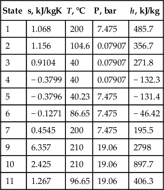
The energy efficiency of this cycle is 24%, the exergy efficiency is 15%, and the Carnot efficiency calculated with the maximum temperature of geothermal brine is 38%. If the pressure of the geothermal brine is high enough, then steam-flash power plant cycles can be an effective solution for power generation.

Figure 7.52 presents two types of flash power plants, namely single-flash and double-flash kinds. In these systems, high-pressure geothermal brine is flashed at an intermediate pressure through an isenthalpic process (1–2). Thus saturated vapor flashes from the liquid and is directed toward the turbine. There it is expanded to low pressure and then condensed using heat sink as the ambient. After condensation, the resulting water is reinjected into the well. Note also that the steam resulting from flashing can be used for other processes than power generation. For instance it can be used to produce refrigeration, using ejectors in a refrigeration cycle. The double-flash cycle can be applied if the moisture content of the expanded steam is too high; this is done by expanding in two stages.

Another effective option for geothermal fields that generate high-pressure brine is the flash-binary power plant. This kind of power plant couples a flash cycle which operates with the geothermal brine as working fluid with a bottoming ORC in the way illustrated in Figure 7.53. After the flashing process, the steam is expanded in a turbine, while the resulting liquid is passed through a heat exchanger which preheats and boils the working fluid of the bottoming cycle. The system has two independent condensers. It is important to match the temperature profiles in the heat exchanger such that the available exergy is exploited at maximum benefit for improved system performance.

7.5 Biomass Energy Systems

Any kind of fossilized living species is a form of biomass. It is one of the oldest energy sources on the earth and may become one of the most significant large-scale energy sources in the future. Biomass originates from the photosynthesis aspect of solar energy distribution and includes all plant life (terrestrial and marine), all subsequent species in the food chain, and eventually all organic waste. Biomass resources come in a large variety of wood forms, crop forms, and waste forms. The basic characteristic of biomass is its chemical composition, in such forms as sugar, starch, cellulose, hemicellulose, lignin, resins, and tannins.

Bioenergy (or biomass energy) may be defined as the energy extracted from biomass for conversion into a useful form for commercial heat, electricity, and transportation fuel applications. The simplest route to biomass energy conversion is by combustion to generate heat. The high-temperature heat can be further converted into work through heat engines. Other biomass conversion routes are illustrated in Figure 7.54. This combustion is a thermochemical process where it is called as gasification. Gasification converts the biomass into a gaseous fuel. Liquefaction produces a liquid fuel. Another route of biomass energy conversion is biochemical. In this case, the fermentation process (anaerobic or aerobic digestion) can lead to biogas, alcohol, and hydrogen generation. Also, the photosynthesis process conducted by some phototrophic organisms can eventually produce hydrogen.

Because energy crop fuel contains almost no sulfur and has significantly less nitrogen than fossil fuels (reducing pollutants causing acid rain [SO₂] and smog [NO_x]), its use will improve our air quality. An additional environmental benefit is in water quality, as energy crop fuel contains less (to none) mercury than coal. Also, energy crop farms using environmentally proactive designs will create water quality filtration zones, taking up and sequestering pollutants (e.g., phosphorus from soils that leach into water bodies).

Biomass generates about the same amount of CO₂ as do fossil fuels (when burned), but from a chemical balance point of view, every time a new plant grows CO₂ is actually removed from the atmosphere. The net emission of CO₂ will be zero as long as plants continue to be replenished for biomass energy purposes. If the biomass is converted through gasification or pyrolysis, the net balance can even result in removal of CO₂. Energy crops such as fast-growing trees and grasses are called biomass feedstocks. The use of biomass feedstocks can help increase profits for the agricultural industry.

The general model of biomass energy conversion into work consists of an adiabatic combustor and a reversible heat engine. Figure 7.55 shows a temperature versus air–fuel ratio (AFR) diagram for thermochemical conversion of biomass. Depending on temperature and the AFR the process used can be combustion, gasification, or pyrolysis. The biomass combusts in an adiabatic combustor which operates at the highest possible temperature (T_ad). The heat generated in this process is the net calorific value of the biomass (NCV).

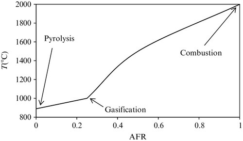
The work generated by this system is thus $\dot{\mathit{W}}=\mathit{N}\mathit{C}\mathit{V}(1-{\mathit{T}}_0/{\mathit{T}}_{\mathrm{ad}})$, and the efficiency of the biomass conversion process is given by the adiabatic flame temperature only, η = 1 − T₀/T_ad. Therefore, determining the thermodynamic limit of biomass energy conversion is equivalent to determining the adiabatic flame temperature for the biomass. We will analyze the biomass composition and the way in which this affects the net calorific value of biomass and the corresponding adiabatic flame temperature.

The biomass contains various biochemicals (amino acids, fiber, cellulose, sugars, glucose, and many others). Some living microorganisms and enzymes may be found in biomass. The most abundant chemical elements in biomass are carbon, hydrogen, oxygen, nitrogen, and sulfur. Other elements are also present, including metal atoms. When biomass is combusted, the metal atoms and other elements form ash.

The general chemical model of biomass is written as ${\mathrm{C}}_{{\mathit{X}}_{\mathrm{C}}}{\mathrm{H}}_{{\mathit{X}}_{\mathrm{H}}}{\mathrm{O}}_{{\mathit{X}}_{\mathrm{O}}}{\mathrm{N}}_{{\mathit{X}}_{\mathrm{N}}}{\mathrm{S}}_{{\mathrm{X}}_{\mathrm{S}}}{\mathrm{ash}}_{{\mathit{X}}_{\mathrm{ash}}}{\left({\mathrm{H}}_2\mathrm{O}\right)}_{{\mathit{X}}_{\mathrm{w}}}$ where X_i is the number of constituents of species “i.” If the moisture (water) is eliminated by a drying process, then the chemical representation of the dry biomass becomes ${\mathrm{C}}_{{\mathit{X}}_{\mathrm{C}}}{\mathrm{H}}_{{\mathit{X}}_{\mathrm{H}}}{\mathrm{O}}_{{\mathit{X}}_{\mathrm{O}}}{\mathrm{N}}_{{\mathit{X}}_{\mathrm{N}}}{\mathrm{S}}_{{\mathit{X}}_{\mathrm{S}}}{\mathrm{ash}}_{{\mathit{X}}_{\mathrm{ash}}}$. The molecular mass of dry biomass can be calculated with

$\mathit{M}=12\times {\mathit{X}}_{\mathrm{C}}+{\mathit{X}}_{\mathrm{H}}+16\times {\mathit{X}}_{\mathrm{O}}+14\times {\mathit{X}}_{\mathrm{N}}+32\times {\mathit{X}}_{\mathrm{S}}+{\mathit{M}}_{\mathrm{ash}}{\mathit{X}}_{\mathrm{ash}}$

On a dry basis, the mass concentration of each major chemical element constituent is ${\mathit{w}}_{\mathrm{C}}=12\times \frac{{\mathit{X}}_{\mathrm{C}}}{\mathit{M}};{\mathit{w}}_{\mathrm{H}}=\frac{{\mathit{X}}_{\mathrm{H}}}{\mathit{M}};{\mathit{w}}_{\mathrm{O}}=16\times \frac{{\mathit{X}}_{\mathrm{O}}}{\mathit{M}};{\mathit{w}}_{\mathrm{N}}=14\times \frac{{\mathit{X}}_{\mathrm{N}}}{\mathit{M}};{\mathit{w}}_{\mathrm{S}}=32\times \frac{{\mathit{X}}_{\mathrm{S}}}{\mathit{M}};{\mathit{w}}_{\mathrm{ash}}={\mathit{M}}_{\mathrm{ash}}\times \frac{{\mathit{X}}_{\mathrm{ash}}}{\mathit{M}}$, where w_ash = 0.5 − 12% dry basis. The moisture content of biomass typically has a moisture concentration in the range w_w = 0 − 50% and can be expressed on wet basis as

${\mathit{M}}_{\mathrm{wet}}=\mathit{M}+{\mathit{X}}_{\mathrm{w}}\times 18$

Thus,

${\mathit{w}}_{\mathrm{w}}=\frac{18{\mathit{X}}_{\mathrm{w}}}{\mathit{M}+{\mathit{X}}_{\mathrm{w}}\times 18}$

If the mass concentration of the moisture is known, then the molar concentration can be determined with

${\mathit{X}}_{\mathrm{w}}=\frac{{\mathit{w}}_{\mathrm{w}}\mathit{M}}{18\left(1-{\mathit{w}}_{\mathrm{w}}\right)}$

The general chemical equation of biomass combustion with enriched oxygen and flue gas recirculation is ${\mathrm{C}}_{{\mathit{X}}_{\mathrm{C}}}{\mathrm{H}}_{{\mathit{X}}_{\mathrm{H}}}{\mathrm{O}}_{{\mathit{X}}_{\mathrm{O}}}{\mathrm{N}}_{{\mathit{X}}_{\mathrm{N}}}{\mathrm{S}}_{{\mathrm{X}}_{\mathrm{S}}}{\mathrm{ash}}_{{\mathit{X}}_{\mathrm{ash}}}{\left({\mathrm{H}}_2\mathrm{O}\right)}_{{\mathit{X}}_{\mathrm{w}}}+\mathit{\lambda }{\mathit{X}}_{{\mathrm{O}}_2}\left[\mathit{\zeta }\left({\mathrm{O}}_2+3.76{\mathrm{N}}_2\right)+\left(\mathit{\zeta }-1\right){\mathrm{O}}_2\right]\to \mathrm{P}\mathrm{r}\mathrm{o}\mathrm{d}+{\mathit{X}}_{\mathrm{ash}}\mathrm{a}\mathrm{s}\mathrm{h}$, where λ ≥ 1 is the excess oxygen,3.76 is the concentration of nitrogen in fresh air, ζ = 0 − 1 is the fraction of fresh air, and “Prod”represents the reaction products in the form of flue gas. Assuming complete combustion one has: $\mathrm{P}\mathrm{r}\mathrm{o}\mathrm{d}={\mathit{X}}_{\mathrm{C}}{\mathrm{CO}}_2+{\mathit{X}}_{{\mathrm{H}}_2\mathrm{O}}{\mathrm{H}}_2\mathrm{O}+{\mathit{X}}_{\mathrm{S}}{\mathrm{SO}}_2+{\mathit{X}}_{{\mathrm{N}}_2}{\mathrm{N}}_2+\left(\mathrm{\lambda }-1\right){\mathit{X}}_{{\mathrm{O}}_2}{\mathrm{O}}_2$, where the stoichiometric coefficient for nitrogen is ${\mathit{X}}_{{\mathrm{N}}_2}={\mathit{X}}_{\mathrm{N}}/2+3.76\mathit{\lambda }\mathit{\zeta }{\mathit{X}}_{{\mathrm{O}}_2}$.

The plot in Figure 7.56 illustrates the variation of adiabatic flame temperature and conversion efficiency of a typical biomass with the moisture content. The energy and exergy efficiencies are calculated based on useful work generated and the energy and exergy input.

The maximum conversion efficiencies are obtained with dry biomass (moisture content 0%) and excess oxidant (air) as low as stoichiometric 1 (λ = 1). In these conditions the adiabatic flame temperature as well as the maximum biomass energy conversion efficiencies reach values around T_ad = 1280 − 1300 °C, η ≅ 80%, and ψ ≅ 72%. Table 9.13 gives the characterization of some biomass resources.

Biomass can be converted to a gaseous fuel by two routes, namely the thermochemical and biochemical conversion routes. Through the thermochemical conversion route bio-syngas is obtained, while by biochemical conversion one can generate either biogas or hydrogen.

Several alternatives are available for generation of electric power from biomass. The simplest way to do this is by direct combustion of biomass, firing a steam generator which drives a turbine. Biomass combustion facilities can be also coupled with ORCs which are characterized by good turbine efficiency at low installed capacities.

When biomass is converted to biogas, then electric power generators based on internal combustion engines can be used for power production. It is also possible to couple biogas production facilities with micro-power plants comprising gas turbines cascaded with a reciprocating internal combustion engine. For micro-power plants, alcohol and gasoline motors can be operated with methane without affecting their operational integrity. This adaptation is made by installing a cylinder of biogas in place of conventional fuel. For gas flow regulation, a reducer is placed close to the motor.

The combined heat and power generation (via biomass gasification techniques connected to gas-fired engines or gas turbines) can achieve significantly higher electrical efficiencies, between 22% and 37%, than those of biomass combustion technologies with steam generation and a steam turbine, 15–18%. If the gas produced is used in fuel cells for power generation, an even higher overall electrical efficiency can be attained, in the range of 25–50%, even in small-scale biomass gasification plants and under partial load operation.

Due to the improved electrical efficiency of energy conversion via gasification, the potential reduction in CO₂ is greater than with combustion. The formation of NO_x compounds can also be largely prevented, and the removal of pollutants is easier for various substances. The NO_x advantage, however, may be partly lost if the gas is subsequently used in gas-fired engines or gas turbines. Significantly lower emissions of NO_x, CO, and hydrocarbons can be expected when the gas produced is used in fuel cells rather than gas-fired engines or gas turbines.

Figure 7.57 shows a biomass gasifier where a gas production module converts biomass to a clean gas for power and steam generation with a combined Brayton cycle, steam expansion turbine, and fuel cell. In this system, biomass is gasified first and then used in a gas turbine and a fuel cell system that operate in parallel. The un-combusted gases are directed toward a low-pressure combustor where additional combustion is applied at low pressure. The flue gases are used to generate high-pressure superheated steam that is expanded in a steam turbine. The resulting low-pressure steam can be used for some heating applications. Another part of the high-pressure steam is used for the gasification process.

7.6 Ocean Energy Systems

The ability to directly extract energy from the world’s oceans comes in four forms: tides, waves, ocean currents, and thermal energy. When tides come into the shore, they can be trapped in reservoirs behind dams. Then when the tide drops, the water behind the dam can be released just as in a regular hydroelectric power plant. Tidal energy shows good potential for electric energy generation. A classification of ocean energy conversion options for power generation is illustrated in Figure 7.58.

The kinetic energy resulting from the moon’s (in addition to the sun’s smaller) gravitational pull on the oceans during the earth’s rotation, producing a diurnal tidal effect, creates the potential to utilize the kinetic energy of waves hitting continental shores for power generation. Wave energy can be collected with floating bodies that execute elliptic movement under the action of waves.

The heat cycle of tropical solar energy affects the oceans during the earth’s rotation and generates kinetic energy that can be used directly to turn submerged turbine generators. The temperature gradient of the ocean with depth results in a temperature difference just large enough over reasonable depths to extract thermal energy at low efficiency. This is called ocean thermal energy conversion. Ammonia-water Rankine and Kalina cycles have been proposed for OTEC. Using depth seawater temperature as a sink at 4 °C, and the ambient temperature at 25–35 °C as a heat source, energy efficiency of about 5% can be obtained.

An OTEC system configuration is illustrated in Figure 7.59. The system is basically a Rankine cycle operating with ammonia as the working fluid. The system can be installed on a floating platform or on a ship. It uses the surface water as the source. Normally the water at ocean surface is at a higher temperature than in deep ocean. The surface water is circulated with pumps through a heat exchanger which acts as a boiler for ammonia. Water from deep ocean at 4 °C is pumped to the surface and used as heat sink in an ammonia condenser.

Apart from being an immensely large thermal energy storage system (which is an indirect form of solar energy storage), oceans are at the same time huge reservoirs of mechanical energy. This mechanical energy manifests in the form of tides, ocean currents, and ocean waves. The kinetic energy resulting from the moon’s (in addition to the sun’s smaller) gravitational pull on the oceans during the earth’s rotation produces a diurnal tidal effect. The formation of tides is explained in Figure 7.60. Basically two bulges of water are formed at the equatorial belt due to the combined action of gravitational and centrifugal forces. Tidal energy shows good potential for electric energy generation. The associated energy can be converted into electricity by two methods:

• Generation of a difference in water level through impoundment. When tides come into the shore, they can be trapped in reservoirs behind dams. Then when the tide drops, the water behind the dam can be let out as in a regular hydroelectric power plant. As the tidal water level difference is rather small, Kaplan turbines are mostly used to generate power.

• Momentum transfer between the currents generated by tides and a conversion device like a water turbine. Ocean current harvesting systems are used to rotate propellers that are coupled to electric generators.

A tidal impoundment (barrage) system can have three methods of operation, depending on the phase at which it generates power: ebb generation, flood generation, and two-way generation. When ebb generation is applied the basin is filled during the flood tide. During the night additional water can be pumped into the basin, as a means of energy storage during off-peak hours. When the tide ebbs low enough, water is discharged over turbine systems which generate power. In flood generation, the dam gates are closed such that the water level increases on the ocean side until it reaches the maximum. Then water is allowed to flow through turbine systems and fill the basin while generating power. In two-way generation, electricity is generated in both the flood and ebb phases of the tide. In Table 7.16 some of the main tidal power generation systems that have been built and their principal characteristics are listed. The world largest tidal power generation site is in France at “La Rance,” with an installed capacity of 240 MW, operating with 24 reversible turbines and a hydrostatic head of 5 m.

Ocean water currents are generated by tides, the earth spinning, the heat cycle of tropical solar energy,and superficial winds. The water current energy can be extracted through current turbines submerged in water. Basically, water current turbines are similar to wind turbines, with the difference that the density and the viscosity of water are 100 and 1000 times higher than that of air, respectively. Therefore, there are some differences between the operation of water current turbines and wind turbines. As for wind turbines, water current turbines are made with horizontal axis or vertical axis construction. The thrust generated by water current turbines is much higher than that specific to wind turbines. Therefore, their construction material must be more massive and resistant.

Surface winds, tides, and ocean currents contribute to the formation of ocean waves. The energy of waves can be collected with floating bodies that execute elliptic movement under the action of gravity and wave motion. The wave energy can be measured in terms of wave power per meter of wave front. The highest wave power on the globe appears to be in southern Argentina across the Strait of Magellan, where wave power density can reach 97 kW/m. Also, along the southwestern coast of South America, the wave power density is over 50 kW/m and often over 70 kW/m. On southwestern Australian coasts, the wave power reaches 78 kW/m. In the northern hemisphere, the highest wave intensity if found along the coast of western Ireland and the UK, with magnitudes around 70 kW/m. The southern coast of Alaska records wave power density up to 65–67 kW/m. The wave power density in other coastal regions varies from about 10–50 kW/m. This impressive amount of energy can be converted to electricity with relatively simple mechanical systems that can be classified as one of two kinds, buoy type or turbine type.

The principle schematic of a buoy-type wave energy converter is suggested in Figure 7.61 and operates based on hydraulic-pneumatic systems. The buoy oscillates according to the wave movement at the ocean surface. It transmits the reciprocating movement to a double-effect hydraulic pump which is anchored rigidly on the ocean bottom. The pump generates a pressure difference between two pneumatic-hydraulic cylinders. A hydraulic motor generates shaft work by discharging the high-pressure liquid into a low-pressure reservoir. The shaft work turns an electric generator which produces electricity.

The energy of waves is correlated with the energy of surface winds. Two aspects are important in determining the interrelation between the wave height and the wind characteristics, namely the wind-water fetch (that is, the length over which the superficial wind contacts the water) and the duration of the wind. For example, if the wind blows constantly for 30 h at 30 km/h and is in contact with water over a length of 1200 km, the wave height can reach 20 m (see Da Rosa, 2009). The power density of the wave in deep ocean water can be approximated with

$\dot{\mathit{W}}=0.5\mathit{v}\mathit{\rho }\mathit{g}{\mathit{h}}^2$

while in shallow waters it is about half of this. In the equation, v is the eave speed, ρ is the water density, g = 9.81 m/s² is the gravity acceleration, and h is the height of the wave. Thus a 10-m wave propagating at 1 m/s carries a power density of 49 kW/m.

If the waves are high, an arrangement can be made in such a way that a difference of level is created constantly through impoundment. Thus the top of the wave carries waters over the impoundment, constantly filling a small basin at higher water level. The difference in water levels is turned into shaft work by a Kaplan turbine system.

Osmotic energy technology uses the energy available from the different salt concentrations in seawater and freshwater. Such resources are found in large river estuaries and fjords. The system uses a semi-permeable membrane that allows the salt concentrations to equalize, thus increasing pressure in the seawater compartment. The technology is still in early research and development stages (Achilli et al., 2009). Statkraft (2013) is one of the few industrial players in this sector, having set up the world’s first prototype osmotic power plant in Norway. The key to further development lies in optimizing membrane characteristics. Today, the membranes generate only a few watts per square meter. The small number of players working on this technology and the need to improve membrane performance and reduce costs point to development prospects in the longer term. Research and development on osmotic power is also being carried out at the Tokyo Institute of Technology to develop new efficient membranes, and by RedStack in the Netherlands.

An osmotic power plant extracts power from salinity gradients by guiding freshwater and salt water into separate chambers, divided by a membrane. The salt molecules pull the freshwater through the membrane, creating a pressure on the salt-water side that can drive a turbine. Salinity gradients can also supply power through reversed electrodialysis (RED).

7.7 Concluding Remarks

In this chapter, we introduce renewable-energy-based power generation systems and discuss them for various options of power generation with numerous applications. We address the performance-related issues and explain how to assess the performance of such systems and applications through energy and exergy efficiencies. The available technologies for converting renewable energies into power are analyzed for each case. Numerous illustrative examples and cases studies are presented to highlight the importance of power system design, analysis, and assessment.