Advanced Power Generation Systems

Search in book...
Toggle Font Controls
Create new playlist

Name your new playlist

Playlist description (optional)
Sign In

Email address

Password

Forgot Password?

or

Continue with Facebook

Continue with Google
Sign Up

Full Name

Email address

Confirm Email Address

Password

or

Continue with Facebook

Continue with Google

5.2.5 Steam Rankine Power Stations

5.2.5.1 Reheating-Regenerative Steam Rankine Cycle

The vast majority of power stations are based on reheating-regenerative steam Rankine cycles. These types of cycles are very complex as they comprise many types of components, including preheater, boiler, superheater, reheater, closed (CFWH) and open (OFWH) feedwater heaters, mixer, condenser, deaerator, pumps, and steam traps (ST). The cycle design depends on the type of heat source and heat sink. For most cases of large power generation the heat source is derived from coal combustion.

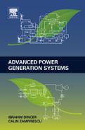
The heat sink is in general a lake; however, there are many cases in which power plants use air as a heat sink. In this case the plant is equipped with cooling towers—either with natural convection or with forced convection. In some situations (e.g., in colder regions) the heat sink is represented by a district heating system for cogeneration. In this section we give an illustrative example of a reheating-regenerative steam Rankine cycle as presented in Figure 5.23. This power plant comprises eighteen main components. There are also four steam extraction ports with corresponding steam extraction fractions denoted with f₁₂, f₁₇, f₂₀, f₂₁. The thermodynamic analysis of the cycle becomes complex because multiple variables and equations are involved and optimization is required for energy efficiency maximization. We will illustrate in detail how the cycle can be analyzed using balance equations and how the optimization problem for maximum efficiency can be formulated.

f05-23-9780123838605 — Figure 5.23 Rankine power plant with single reheating and multiple feedwater heaters (M, mixer; CFWH, closed feedwater heater; OWFH, open feedwater heater; ST, steam trap).

Mass, energy, entropy and exergy balance equations must be written for each component of the power plant in order to form a system of equations that can be solved to determine thermodynamic parameters defining each state. The following observation is very useful for simplifying the mass balance equations: in state 11 (turbine inlet) the mass flow rate is the maximum for the plant; also ${\dot{m}}_{11} = {\dot{m}}_{10} = {\dot{m}}_{9} = {\dot{m}}_{8}$ ${\dot{m}}_{11} = {\dot{m}}_{10} = {\dot{m}}_{9} = {\dot{m}}_{8}$ . Hence, the steam injection fractions are defined with respect to ${\dot{m}}_{11}$ ${\dot{m}}_{11}$ as follows:

$f_{12} {\dot{m}}_{11} = {\dot{m}}_{12}, f_{17} {\dot{m}}_{11} = {\dot{m}}_{17}, f_{20} {\dot{m}}_{11} = {\dot{m}}_{20}, f_{21} {\dot{m}}_{11} = {\dot{m}}_{21}$ $f_{12} {\dot{m}}_{11} = {\dot{m}}_{12}, f_{17} {\dot{m}}_{11} = {\dot{m}}_{17}, f_{20} {\dot{m}}_{11} = {\dot{m}}_{20}, f_{21} {\dot{m}}_{11} = {\dot{m}}_{21}$

In addition, in Figure 5.23 it can be observed that mass balance equations can be reduced to the following set of equations expressed as a function of flow fractions in other state points of the power plant, defined by $f_{i} {\dot{m}}_{11} = {\dot{m}}_{i}$ $f_{i} {\dot{m}}_{11} = {\dot{m}}_{i}$ , namely:

$f_{1} = f_{2} = f_{3} = f_{26}; f_{4} = f_{5} = f_{6} = f_{7}; f_{12} = f_{13} = f_{14}; f_{17} = f_{18} = f_{19}; f_{21} = f_{22} = f_{23}$ $f_{1} = f_{2} = f_{3} = f_{26}; f_{4} = f_{5} = f_{6} = f_{7}; f_{12} = f_{13} = f_{14}; f_{17} = f_{18} = f_{19}; f_{21} = f_{22} = f_{23}$

$f_{15} = f_{16}; f_{24} = f_{25}; f_{25} + f_{23} = f_{26}; f_{12} + f_{15} = 1; f_{4} = f_{15}; f_{16} = f_{17} + f_{20} + f_{21} + f_{24}$ $f_{15} = f_{16}; f_{24} = f_{25}; f_{25} + f_{23} = f_{26}; f_{12} + f_{15} = 1; f_{4} = f_{15}; f_{16} = f_{17} + f_{20} + f_{21} + f_{24}$

Using the flow fractions f_i, the energy, entropy, and exergy balance equations are written for each component as indicated in Table 5.11. The balance equations together with the parameters that quantify exergy destructions (e.g., isentropic efficiencies of pumps and turbines, temperature differences due to heat transfer) form a closed system of equations which can be solved for temperatures, pressures, and specific enthalpy, entropy, and volume at each state point provided that all extraction fractions are specified (f₁₂, f₁₇, f₂₀, f₂₁) and the condensation, boiling, and superheating temperatures (T₁, T₉, T₁₁) are given.

Table 5.11

Balance Equations for Ideal Rankine Cycle of Power Plant in Figure 5.23

Component	Equations	Component	Equations
Pump 1 (states 1–2)	MBE: ${\dot{m}}_{1} = {\dot{m}}_{2}$ ${\dot{m}}_{1} = {\dot{m}}_{2}$ EBE: f₁h₁ + w_p1 = f₁h₂ EnBE: s₁ + s_g = s₂ ExBE: f₁ex₁ + w_p1 = f₁ex₂ + ex_d	CFWH1 (states 2–3)	MBE: ${\dot{m}}_{2} = {\dot{m}}_{3}$ ${\dot{m}}_{2} = {\dot{m}}_{3}$ EBE: f₁h₂ + f₂₁h₂₁ = f₁h₃ + f₂₁h₂₂ EnBE: f₁s₂ + f₂₁s₂₁ + s_g = f₁s₃ + f₂₁s₂₂ ExBE: f₁ex₂ + f₂₁ex₂₁ = f₁ex₃ + f₂₁ex₂₂ + ex_d
Pump 2 (states 4–5)	MBE: ${\dot{m}}_{4} = {\dot{m}}_{5}$ ${\dot{m}}_{4} = {\dot{m}}_{5}$ EBE: f₄h₄ + w_p2 = f₄h₅ EnBE: s₄ + s_g = s₅ ExBE: f₄ex₄ + w_p2 = f₄ex₅ + ex_d	OFWH (states 3–4–19–20)	MBE: $f_{1} {\dot{m}}_{11} + f_{17} {\dot{m}}_{11} + f_{20} {\dot{m}}_{11} = f_{4} {\dot{m}}_{11}$ $f_{1} {\dot{m}}_{11} + f_{17} {\dot{m}}_{11} + f_{20} {\dot{m}}_{11} = f_{4} {\dot{m}}_{11}$ EBE:f₁h₃ + f₁₇h₁₈ + f₂₀h₂₀ = f₄h₄ EnBE: f₁s₃ + f₁₇s₁₈ + f₂₀s₂₀ + s_g = f₄s₄ ExBe: f₁ex₃ + f₁₇ex₁₈ + f₂₀ex₂₀ = f₄ex₄ + ex_d
Pump 3 (states 13–14)	MBE: ${\dot{m}}_{13} = {\dot{m}}_{14}$ ${\dot{m}}_{13} = {\dot{m}}_{14}$ EBE: f₁₂h₁₃ + w_p3 = f₁₂h₅ EnBE: s₁₃ + s_g = s₁₄ ExBE: f₁₂ex₁₃ + w_p3 = f₁₂ex₁₃ + ex_d	CFWH2 (states 5–6–17–18)	MBE: $f_{4} {\dot{m}}_{11} + f_{17} {\dot{m}}_{11} = f_{4} {\dot{m}}_{11} + f_{17} {\dot{m}}_{11}$ $f_{4} {\dot{m}}_{11} + f_{17} {\dot{m}}_{11} = f_{4} {\dot{m}}_{11} + f_{17} {\dot{m}}_{11}$ EBE: f₄h₅ + f₁₇h₁₇ = f₄h₆ + f₁₇h₁₈ EnBE: f₄s₅ + f₁₇s₁₇ + s_g = f₄s₆ + f₁₇s₁₈ ExBE: f₄ex₅ + f₁₇ex₁₇ = f₄ex₆ + f₁₇ex₁₈ + ex_d
Mixer (states 7–8–14)	MBE: $f_{4} {\dot{m}}_{11} + f_{12} {\dot{m}}_{11} = f_{8} {\dot{m}}_{11}$ $f_{4} {\dot{m}}_{11} + f_{12} {\dot{m}}_{11} = f_{8} {\dot{m}}_{11}$ EBE: f₄h₇ + f₁₂h₁₄ = h₈ EnBE: f₄s₇ + f₁₂s₁₄ + s_g = s₈ ExBE: f₄ex₇ + f₁₂ex₁₄ = ex₈ + ex_d	CFWH3 (states 6–7–12–13)	MBE: $f_{4} {\dot{m}}_{11} + f_{12} {\dot{m}}_{11} = f_{4} {\dot{m}}_{11} + f_{12} {\dot{m}}_{11}$ $f_{4} {\dot{m}}_{11} + f_{12} {\dot{m}}_{11} = f_{4} {\dot{m}}_{11} + f_{12} {\dot{m}}_{11}$ EBE: f₄h₆ + f₁₂h₁₂ = f₄h₇ + f₁₂h₁₃ EnBE: f₄s₆ + f₁₂s₁₂ + s_g = f₄s₇ + f₁₂s₁₃ ExBE: f₄ex₆ + f₁₂ex₁₂ = f₄ex₇ + f₁₂ex₁₃ + ex_d
Preheater (states 8–9)	MBE: ${\dot{m}}_{8} = {\dot{m}}_{9}$ ${\dot{m}}_{8} = {\dot{m}}_{9}$ EBE: h₈ + q_ph = h₉ EnBE: s₈ + q_ph/T_ph + s_g = s₉ ExBE: ex₈ + q_ph(1 − T₀/T_ph) = ex₉ + ex_d	Boiler (states 9–10)	MBE: ${\dot{m}}_{9} = {\dot{m}}_{10}$ ${\dot{m}}_{9} = {\dot{m}}_{10}$ EBE: h₉ + q_b = h₁₀ EnBE: s₉ + q_b/T_b + s_g = s₁₀ ExBE: ex₉ + q_b(1 − T₀/T_b) = ex₁₀ + ex_d
Superheater (states 10–11)	MBE: ${\dot{m}}_{10} = {\dot{m}}_{11}$ ${\dot{m}}_{10} = {\dot{m}}_{11}$ EBE: h₁₀ + q_sh = h₁₁ EnBE: s₁₀ + q_sh/T_sh + s_g = s₁₁ ExBE: ex₁₀ + q_sh(1 − T₀/T_sh) = ex₁₁ + ex_d	Reheater (states 15–16)	MBE: ${\dot{m}}_{15} = {\dot{m}}_{16}$ ${\dot{m}}_{15} = {\dot{m}}_{16}$ EBE: f₁₅h₁₅ + q_rh = f₁₅h₁₆ EnBE: f₁₅s₁₅ + q_rh/T_sh + s_g = f₁₅s₁₆ ExBE: f₁₅ex₁₅ + q_rh(1 − T₀/T_rh) = f₁₅ex₁₆ + ex_d
Turbine 1 (states 11–12–15)	MBE: ${\dot{m}}_{11} = {\dot{m}}_{12} + {\dot{m}}_{15}$ ${\dot{m}}_{11} = {\dot{m}}_{12} + {\dot{m}}_{15}$ EBE: h₁₁ = f₁₂h₁₂ + f₁₅h₁₅ + w_t1 EnBE:s₁₁ + s_g = f₁₂s₁₂ + f₁₅s₁₅ ExBE: ex₁₁ = f₁₂ex₁₂ + f₁₅ex₁₅ + w_t1 + ex_d	Turbine 2 (states 16–17–20–21–24)	MBE: f₁₅ = f₁₇ + f₂₀ + f₂₁ + f₂₄; EBE: f₁₅h₁₆ = f₁₇h₁₇ + f₂₀h₂₀ + f₂₁h₂₁ + f₂₄h₂₄ + w_t2; EnBE: f₁₅s₁₅ + s_g = f₁₇s₁₇ + f₂₀s₂₀ + f₂₁s₂₁ + f₂₄s₂₄; ExBE: $\begin{array}{l} f_{15} e x_{15} = f_{17} e x_{17} + f_{20} e x_{20} \\ + f_{21} e x_{21} + f_{24} e x_{24} + w_{t 2} + e x_{d} \end{array}$ $\begin{array}{l} f_{15} e x_{15} = f_{17} e x_{17} + f_{20} e x_{20} \\ + f_{21} e x_{21} + f_{24} e x_{24} + w_{t 2} + e x_{d} \end{array}$
ST 1 (states 22–23)	MBE: ${\dot{m}}_{22} = {\dot{m}}_{23}$ ${\dot{m}}_{22} = {\dot{m}}_{23}$ EBE: h₂₂ = h₂₃ EnBE: f₂₁s₂₂ + s_g = f₂₁s₂₃ ExBE: f₂₁ex₂₂ = f₂₁ex₂₃ + ex_d	ST 2 (states 18–19)	MBE: ${\dot{m}}_{18} = {\dot{m}}_{19}$ ${\dot{m}}_{18} = {\dot{m}}_{19}$ EBE: h₁₈ = h₁₉ EnBE: f₁₇s₁₈ + s_g = f₁₇s₁₉ ExBE: f₁₇ex₁₈ = f₁₇ex₁₉ + ex_d

t0060

As seen in Table 5.11 the balance equations can be written using mass-specific quantities. These quantities are defined with respect to the mass flow rate at the HPT inlet; thus: $w = \dot{W} / {\dot{m}}_{11}$ $w = \dot{W} / {\dot{m}}_{11}$ and $q = \dot{Q} / {\dot{m}}_{11}$ $q = \dot{Q} / {\dot{m}}_{11}$ . Furthermore, the energy efficiency can be maximized according to the following objective function:

$max \{η = \frac{w_{net}}{q_{in}} = F (f_{12}, f_{17}, f_{20}, f_{21}) with given T_{1}, T_{9}, T_{11} and f_{i} \in (0, 1)\}$ $max \{η = \frac{w_{net}}{q_{in}} = F (f_{12}, f_{17}, f_{20}, f_{21}) with given T_{1}, T_{9}, T_{11} and f_{i} \in (0, 1)\}$

si302_e

where F(f₁₂, f₁₇, f₂₀, f₂₁) represents the functional relation between steam extraction fractions and the energy efficiency of the cycle, a relation which is established by the nonlinear system of equations mentioned above.

Note that the certain additional assumptions must be made in order for the optimization problem to be completely specified. These assumptions are as follows:

• at pump suction the liquid is saturated, hence x₁ = x₄ = x₁₃ = 0

• at the steam traps inlet the liquid is saturated, hence x₁₈ = x₂₂ = 0

• at the OFW outlet there is a saturated liquid, hence x₄ = 0

• there is a minimum temperature difference at the closed feedwater heater outlet denoted with ΔT_hx; it is assumed that T₂₂ − T₃ = T₁₈ − T₆ = T₁₃ − T₇ = ΔT_hx.

Example 5.6

Let us consider a steam cycle of the configuration described in Figure 5.23. The following parameters are assumed: T_c = 30 °C; T_b = 293 °C; T_sh = T_rh = 400 °C; ΔT_hx = 10°C, where T_sh and T_rh are the superheating and reheating temperatures, respectively. We want to determine the optimum steam extraction fractions that maximize cycle energy efficiency for two cases: (i) all pumps and turbines operating reversibly and (ii) the isentropic efficiency of the pumps and steam turbines is 0.85. Exergy destructions for each of the components will be determined for case (ii).

The results of the optimization problem (solved with EES software) are presented in Table 5.12 for case (i). We assume that water is saturated liquid at the pump inlet and at closed feedwater heater outlets (states 13, 18, 22). There are optimal values for steam extraction fractions and optimum extraction pressures. It can be observed that the largest extraction is required after the first stage of expansion with f₁₂ = 14.4% and the extraction fraction decreases when decreasing the pressure. The mass-specific net generated work is 1069 kJ/kg while heat input is 2350 kJ/kg.

Table 5.12

Performance Parameters of Optimized Ideal Rankine Cycle of Figure 5.23

Parameter	Value
Parameters with assumed values	T_c = 30 °C; T_b = 293 °C, T_sh = T_rh = 400 °C; ΔT_hx = 10 °C
Optimum extraction fractions	f₁₂ = 14.4%, f₁₇ = 6.7%, f₂₀ = 8.3%, f₂₁ = 5.1%
Optimized extraction pressures	P₁₂ = 3, 381 kPa; P₁₇ = 988 kPa; P₂₀ = 266 kPa; P₂₁ = 39.3 kPa
Energy and exergy efficiencies and Carnot based efficiency	$η = \frac{w_{net}}{q_{in}} = 45.5 %, ψ = \frac{η}{1 - T_{0} / T_{sh}} = 81.6 %$ $η = \frac{w_{net}}{q_{in}} = 45.5 %, ψ = \frac{η}{1 - T_{0} / T_{sh}} = 81.6 %$
Net generated work	w_net = w_t1 + w_t2 − w_p1 − w_p2 − w_p3 = 1, 069 kJ/kg
Heat input and exergy consumed	q_in = h₁₁ − h₈ = 2, 350kJ/kg; ex_cons = ex₁₁ − ex₈ = 885kJ/kg
Exergy destroyed	ex_d = ∑ ex_d = 62.18 kJ/kg; for each component the exergy destruction in percents with respect to total is as follows: ex_d,c = 34%; ex_d,CFWH1 = 12.6% ex_d,CFWH2 = 11.2%; ex_d,CFWH3 = 19.9%; ex_d,M ≅ 0.2%; ex_d,OFWH = 20.1%; ex_d,ST1 = 1.0%; ex_d,ST2 = 1.0%
Pressure ratio over turbines	PR₁ = P₁₁/P₁₂ = 2.3; PR₂ = P₁₆/P₂₄ = 796
Expansion ratio over turbine	$E R_{1} = \frac{v_{12}}{v_{11}} = 1.91; E R_{2} = \frac{v_{24}}{v_{16}} = 300$ $E R_{1} = \frac{v_{12}}{v_{11}} = 1.91; E R_{2} = \frac{v_{24}}{v_{16}} = 300$
Back work ratio	$BWR = \frac{w_{p 1} + w_{p 2} + w_{p 3}}{w_{t 1} + w_{t 2}} = 0.7 %$ $BWR = \frac{w_{p 1} + w_{p 2} + w_{p 3}}{w_{t 1} + w_{t 2}} = 0.7 %$

Note: T_c = T₁; T_b = T₉; T_sh = T_rh = T₁₁.

The energy efficiency (which is maximized) reaches 45.5%. Moreover, one notes that vapor quality at the isentropic turbine outlet is 80%, which is acceptable. The exergy efficiency of the system is exceptionally good, namely ψ = 81.6%, due to the assumed reversible operation of pumps and turbines. Note that the average temperature at the steam generator is approximated to 603.2 K (Carnot factor 50.6%); the Carnot factor associated with the turbine inlet temperature is 55.7%.

The total exergy destruction for case (i) is 61.18 kJ/kg. The highest exergy destruction occurs in the condenser at 34% of total, followed by the OFW and the high-pressure closed feedwater heater CFWH3, each with ~ 20% of total exergy destruction. The exergy destruction in the mixer is negligible.

To solve the cycle in case (ii) the assumption that water is saturated liquid at the pump inlet and at closed feedwater heater outlets is maintained. In addition, the assumption that there is negligible pressure drop in all devices with heat exchange and in pipelines is maintained. Furthermore, for case (ii) temperature differences are assumed for the steam generator as follows: 75 °C for the preheating section, 50 °C for the boiling section, and 25 °C for the superheating and reheating sections.

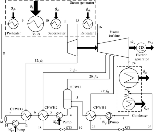
In these conditions the optimum extraction rates are found to have relatively similar values as for case (i), as follows: f₁₂ = 13.3%, f₁₇ = 6.1%, f₂₀ = 7.7%, f₂₁ = 4.8%. The pressure ratio over the HPT is 2.8 and over the LPT is 660. All state point parameters of the optimized cycle are given in Table 5.13. The energy efficiency for case (ii) is degraded to 39.2%, as compared to the case (i) with 45.5%.

Table 5.13

Cycle Parameters of Reheating-Regenerative Steam Rankine Cycle for Case (ii)

State	P (kPa)	T (K)	v (m³/kg)	x (kg/kg)	h (kJ/kg)	s (kJ/kgK)	ex (kJ/kg)	Mass-specific parameters (kJ/kg)
State	P (kPa)	T (K)	v (m³/kg)	x (kg/kg)	h (kJ/kg)	s (kJ/kgK)	ex (kJ/kg)	Component	w	q	ex_d
1	4.246	303.2	0.001004	0	125.7	0.4365	0.1745	Pump 1	0.3	N/A	0.04
2	244.6	303.2	0.001004	− 0.1862	126	0.4367	0.4166	CFWH1	N/A	108	8.05
3	244.6	338.6	0.00102	− 0.1183	274.1	0.8988	10.77	OFWH	N/A	262	12.0
4	244.6	399.9	0.001067	0	532.4	1.6	60.07	Pump 2	8.2	N/A	0.91
5	7769	400.9	0.001063	− 0.5245	541.8	1.603	68.44	CFWH2	N/A	136	6.83
6	7769	437.4	1.977	− 0.417	698.4	1.977	113.6	CFWH3	N/A	256	11.2
7	7769	503.6	0.001203	− 0.2144	993.3	2.604	221.5	M	N/A	N/A	~ 0.0
8	7769	503.8	0.001203	− 0.2138	994.1	2.606	221.8	Preheat.	N/A	312	21.3
9	7769	566.2	0.001377	0	1305	3.187	359.7	Boiler	N/A	1456	62.2
10	7769	566.2	0.02433	1	2761	5.759	1049	Superheat.	N/A	381	7.3
11	7769	673.2	0.03549	1.262	3143	6.382	1245	HPT	213	N/A	20.8
12	2820	546.7	0.08119	100	2930	6.451	1011	Reheater	N/A	264	5.1
13	2820	503.6	0.00121	0	992.3	2.614	217.5	LPT	743	N/A	125.3
14	7769	504.9	0.001205	− 0.2102	999.3	2.616	223.9	Condenser	N/A	1466	24.2
15	2820	546.7	0.08119	1.07	2930	6.451	1011	ST1	N/A	0.0	0.62
16	2820	673.2	0.106	1.238	3234	6.953	1165	ST2	N/A	0.0	0.54
17	877	535.3	0.2736	1.098	2973	7.041	878.4	Cycle parameters
18	877	447.4	0.00112	0	738.1	2.084	121.4	Heat input	q_in = 2, 413 kJ/kg
19	244.6	399.9	0.0701	0.09422	738.1	2.114	112.4	Net work	w_net = 946 kJ/kg
20	244.6	419.3	0.7737	1.019	2757	7.161	626.7	Efficiency	η = 39.2%
21	39.28	348.6	3.845	0.9465	2511	7.319	333.8	Exergy input	ex_in = 1, 253 kJ/kg
22	39.28	348.6	0.001026	0	315.8	1.021	16.1	Efficiency	ψ = 75.5%
23	4.246	303.2	2.575	0.07825	315.8	1.064	3.31	Exergy destruction	ex_d = 306.6 kJ/kg
24	4.246	303.2	29.05	0.883	2271	7.513	35.56	Pressure ratio	HPT: 2.8; LPT: 660

t0070

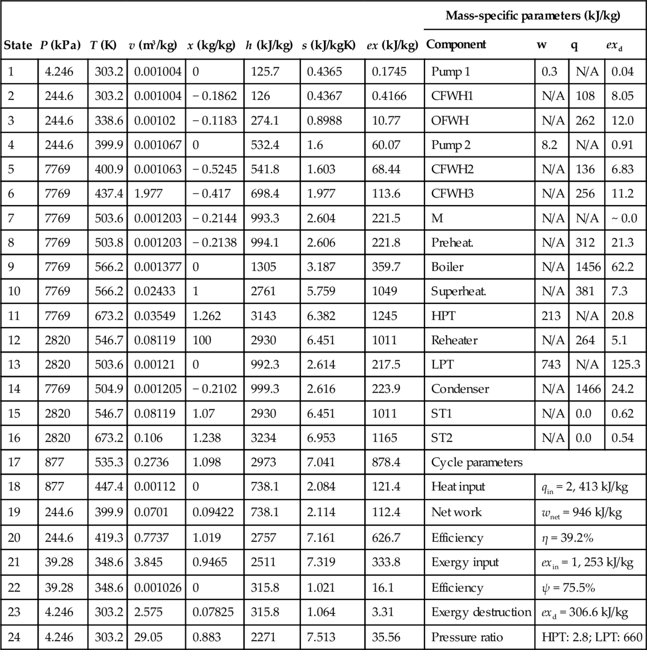
This example underlines the importance of irreversibilities in the steam generator and the turbines. Due to the additional exergy destruction the cycle exergy efficiency for case ii) reduces to 75.5% (for case (i)) the exergy efficiency is 81.6%). The relative exergy destructions for cycle components are represented in the chart in Figure 5.24. Under the assumed conditions the most exergy destruction occurs in the LPT (41%), followed by the steam generator (20%).

f05-24-9780123838605 — Figure 5.24 Exergy destructions for reheating-regenerative cycle in Example 5.6 (case ii).

5.2.5.2 Coal-Fired Power Stations

Although their flue gas stacks highly pollute the atmosphere with carbon dioxide, sulfur dioxide, nitrous oxide emissions, and other pollutants, coal-fired power stations are used in nearly every country of the world. These types of power generating stations are responsible for the majority of global electricity production. They operate based on steam Rankine cycles (generally on reheating-regenerative schemes) and comprise a coal-fired furnace as steam generator.

Two main combustion technologies are used currently in coal-fired power stations, namely pulverized coal boilers (the most predominant) and fluidized bed boilers (used when the coal rank is lower). Although the two technologies are different with regard to transport phenomena, the transient heat and mass transfer from a combusting coal particle to the surroundings are similar in both cases: combustion occurs at the coal particle surface, which gradually consumes while generates incandescent, hot gases. Coal is supplied at the lower part of the furnace where it devolatilizes and ignites in an oxidative atmosphere. The oxygen comes from two sources: fresh air injection and recirculated flue gases. In the first part of the combustion process, the volatiles are oxidized while the temperature of coal particle increases. Thereafter, fixed carbon oxidizes at very fast rate.

In Figure 5.25 the typical configuration of a pulverized coal-fired furnace at a conventional power station is illustrated. It has the roles of preheating, boiling, superheating, and reheating high-pressure steam. The furnace normally is in the form of a tall brick structure of a 10m to 50m height, depending on the type of coal and the residence time of coal particles required for complete combustion. Pulverized coal-fired furnaces are crucial to the utility industry. Typically, pulverized coal-fired furnaces comprise a coal mill which grinds coal to form small powder-like particles conveyed with primary air to the pulverization point, where ignition occurs.

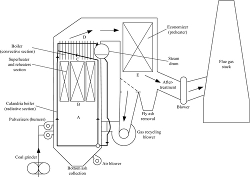
f05-25-9780123838605 — Figure 5.25 Typical coal-fired steam generator configuration for conventional power stations.

The average temperature of gases at the lower part of the pulverized coal furnace (below point A in Figure 5.25) is typically around 650–700 K. A calandria boiler system with vertical tubes is installed at the lower half of the furnace. Between the hot gases inside the furnace duct and the calandria tubes placed at the periphery an intense radiative heat transfer occurs. Under exposure to intense thermal radiation, water boils.

The calandria system comprises a steam drum (see Figure 5.25) which accumulates liquid water at the lower part. Water flows gravitationally downward and feeds into a system formed of multiple headers arranged such that water is distributed uniformly into calandria tubes. The boiling process in the calandira system is incomplete and is facilitated by the fact that the water is close to its saturation state. Given that the boiling water is lighter than the feed water, in the calandria system is formed a natural circulation process due to gravity. In some cases circulation pumps are also used to enhance the water circulation rate.

In later stages of the combustion process, carbon oxidizes and the flue gas temperature increases further. This process occurs approximately between locations A and B in Figure 5.25. At point B, coal particles are completely consumed and the flue gas temperature reaches its maximum value (around 1200 K). In between points B and C the heat of the flue gases is transferred (mainly radiatively) to the superheater and reheaters of the steam Rankine plant. At points C and D there is a heat transfer process by forced convection and radiation between flue gases and the boiling water prior its return to the steam drum. Saturated vapor exists above the liquid in the steam drum. The next heat transfer process in the furnace occurs between D and E where the economizer is installed, which preheats water prior to feeding it into the steam drum. The heat transfer in the economizer is mostly caused by a forced convection process. After point E, a part of the oxygen-containing hot flue gases is returned to the combustion zone in the furnace. Fly ash is removed and electrostatic devices are typically used to remove particulate matter. Further, the flue gases are directed to the stack using a mechanical draft system.

An example of Rankine cycle configuration for a coal-fired steam Rankine power station is shown in Figure 5.26. The system is a double reheating-regenerative Rankine cycle. Liquid water in 1 is pumped by a low-pressure pump (LPP), preheated in a low-pressure closed water-feeding heater (LPFW), further heated in the OFW, and then is pressurized by the high-pressure pump (HPP).

f05-26-9780123838605 — Figure 5.26 Diagram of a coal-fired steam Rankine cycle.

After state 5, pressurized water is the preheated in closed feedwater heater (HPPFW) and in the economizer, and then it is fed as saturated liquid in 7 to the steam drum. Saturated vapor is extracted from the steam drum in 8 and superheated and expanded in the HPT. The expanded steam in 10 is then reheated (RH₁) and expanded in the intermediate-pressure turbine (IPT). The expanded steam in 12 is again reheated (RH₂) and expanded in the LPT. Steam is extracted in 15, 17, 18, and 19 to be used in the water preheating process. In the calandria system, saturated liquid water from the steam drum bottom is extracted in 22 and heated radiatively in the “Calandria HXs” and then further heated by combined convection–radiation heat transfer in the “BOILER” section. The figure illustrates the heat transfer between hot flue gases and steam as shown with bold line. The process B–C represents an approximation of the heat transfer process between the flue gases and the steam at the superheater and the two reheaters. The process C–D represents the heat transfer in the “BOILER” heat exchanger (see Figure 5.26), whereas process D–E represents the heat transfer in the preheater.

The coal type and its specific energy and exergy contents play a role mostly in the design of the furnace and the efficiency of the power plant as well as its air pollution characteristics. The gross calorific value of coal varies from 13 to ~34 MJ/kg; chemical exergy (which is sensitive to moisture content) varies from about 5 to ~25 MJ/kg; and the specific GHG emissions of coal combustion are in the range of 70–140 kg CO₂ equivalent per GJ on a net calorific value basis (see Chapter 3).

For thermodynamic analysis the mass, energy, entropy, and exergy balance must be written for each component of the system. A logical sequence of computation steps requires solving the equations related to coal combustion in the furnace first.

In the actual coal furnace system oxidant in excess is used. Furthermore, additional oxygen is supplied to the combustion process from recirculated flue gases. Therefore, the combustion process can be represented by the following equation

$R + y P + λ x_{st} (O_{2} + 3.76 N_{2}) \to (1 + y) P + a A$ $R + y P + λ x_{st} (O_{2} + 3.76 N_{2}) \to (1 + y) P + a A$

(5.15)

where $R$ $R$ stands for reactant (referring to coal only) and $P$ $P$ for products (except the ash), respectively, $x_{st}$ $x_{st}$ represents the stoichiometric molar fraction of fresh oxygen, λ > 1 is the excess air factor, $y \geq 0$ $y \geq 0$ is the flue gas recycling factor, and $A$ $A$ stands for the ash. It is useful to describe coal using atomic fractions expressed per mole of coal on an as-received basis. Hence, the reactants $R$ $R$ can be represented by the following equation

$R = c C + 0.5 h H_{2} + s S + 0.5 o O_{2} + 0.5 n N_{2} + a A + m H_{2} O$ $R = c C + 0.5 h H_{2} + s S + 0.5 o O_{2} + 0.5 n N_{2} + a A + m H_{2} O$

(5.16)

where $c, h, s, o, n, a, m$ $c, h, s, o, n, a, m$ are determined from weight fractions as-received by dividing with molecular masses.

The reaction products, assuming that complete consumption of coal generates only the products CO₂, H₂O, SO₂, O₂, N₂, and ash, is described by the following equation:

$P = c C O_{2} + (0.5 h + m) H_{2} O + s S O_{2} + (λ - 1) x_{st} O_{2} + (0.5 n + 3.76 λ x_{st}) N_{2}$ $P = c C O_{2} + (0.5 h + m) H_{2} O + s S O_{2} + (λ - 1) x_{st} O_{2} + (0.5 n + 3.76 λ x_{st}) N_{2}$

(5.17)

The stoichiometric molar fraction of fresh air, $x_{st}$ $x_{st}$ , results from atomic species balance:

$x_{st} = c + 0.25 h + s - 0.5 o$ $x_{st} = c + 0.25 h + s - 0.5 o$

(5.18)

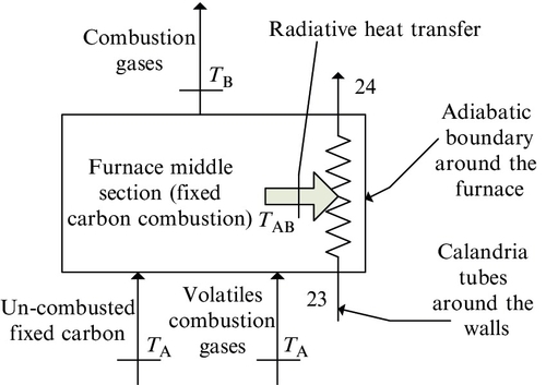
As mentioned above, the first phase of the combustion process is represented by the process of pyrolysis coal and volatile combustion and occurs in a spatial region that extends approximately between the furnace bottom and the coal’s pulverization location. Figure 5.27 gives a sketch representing the matter and heat fluxes in the ignition and volatile combustion zone of the furnace. During the pyrolysis, a series of combustible materials such as long- and short-chain hydrocarbons (e.g., C_nH_2n + 2) and sulfur and some amount of carbon dioxide are released. Hence, a part of fixed carbon is released during pyrolysis as hydrocarbons with a carbon-to-hydrogen ratio of ~0.25–0.47. If one denotes with $z \in (0, 1)$ $z \in (0, 1)$ the fraction of fixed carbon released during pyrolysis, then the volatile combustion phase can be described by the following chemical equation

$R + λ x_{st} (O_{2} + 3.76 N_{2}) + y P \to c (1 - z) C + P_{vc} + a A$ $R + λ x_{st} (O_{2} + 3.76 N_{2}) + y P \to c (1 - z) C + P_{vc} + a A$

(5.19)

where $P_{vc}$ $P_{vc}$ represents the combusted volatile gases defined according to

$P_{vc} = n_{H_{2}} H_{2} + n_{{CO}_{2}} {CO}_{2} + n_{H_{2} O} H_{2} O + n_{{SO}_{2}} S O_{2} + n_{O_{2}} O_{2} + n_{N_{2}} N_{2}$ $P_{vc} = n_{H_{2}} H_{2} + n_{{CO}_{2}} {CO}_{2} + n_{H_{2} O} H_{2} O + n_{{SO}_{2}} S O_{2} + n_{O_{2}} O_{2} + n_{N_{2}} N_{2}$

(5.20)

with

$n_{H_{2}} = 0.5 h (1 - z); n_{{CO}_{2}} = c (z + y); n_{H_{2} O} = 0.5 h (z + y) + m (1 + y); n_{{SO}_{2}} = s (1 + y)$ $n_{H_{2}} = 0.5 h (1 - z); n_{{CO}_{2}} = c (z + y); n_{H_{2} O} = 0.5 h (z + y) + m (1 + y); n_{{SO}_{2}} = s (1 + y)$

$n_{O_{2}} = (1 - z) (c + 0.25 h) + (1 + y) (λ - 1) x_{st}; n_{N_{2}} = (1 + y) (0.5 n + 3.76 λ x_{st})$ $n_{O_{2}} = (1 - z) (c + 0.25 h) + (1 + y) (λ - 1) x_{st}; n_{N_{2}} = (1 + y) (0.5 n + 3.76 λ x_{st})$

standing for the number of moles of components per mole of combusted coal.

f05-27-9780123838605 — Figure 5.27 Representation of ignition zone process and involved streams (furnace bottom).

In the second phase of combustion (see Figure 5.28) the remaining un-combusted fixed carbon from the first phase oxidizes and the temperature of flue gases increases. Recirculated gases are added to the process as a means of adjusting the temperature at the end of combustion phase. The combustion process (see A–B in Figure 5.25) is described by the following equation

$P_{vc} + c (1 - z) C \to (1 + y) P$ $P_{vc} + c (1 - z) C \to (1 + y) P$

(5.21)

f05-28-9780123838605 — Figure 5.28 Representation of fixed carbon combustion process and involved streams.

Notice that the summation of Equation (5.19) and Equation (5.21) gives Equation (5.15), which describes the overall process of coal combustion.

The boiling process continues in the heat exchanger placed between points C and D as indicated in Figure 5.25. Once the thermodynamic states in the furnace (0, A, B, C, D, E, F, 6, 7, 8, 9, 10, 11, 22, 23, 24, 25) are completely determined the analysis proceeds further with balance equations of all other components of the Rankine steam power plant. According to energy balance, the mass flow rate in states 4, 5, 6, 7, 8, 9, and 10 must be the same. According to the overall energy balance on the boiler one has

${\dot{Q}}_{boiler} = {\dot{H}}_{25} - {\dot{H}}_{22} = {\dot{m}}_{7} (h_{8} - h_{7})$ ${\dot{Q}}_{boiler} = {\dot{H}}_{25} - {\dot{H}}_{22} = {\dot{m}}_{7} (h_{8} - h_{7})$

(5.22)

where $\dot{H} = \dot{m} h$ $\dot{H} = \dot{m} h$ is the enthalpy rate of the flow.

In the above equation one accounts for the fact that a saturated liquid enters in state 7 whereas a saturated vapor exits out of the drum in 8. The equation is then solved for ${\dot{m}}_{7}$ ${\dot{m}}_{7}$ . The enthalpy in 25 results from the enthalpy in state 24 and the enthalpies of states C and D on the flue gas side, according to the energy balance

${\dot{H}}_{25} - {\dot{H}}_{24} = {\dot{H}}_{C} - {\dot{H}}_{D}$ ${\dot{H}}_{25} - {\dot{H}}_{24} = {\dot{H}}_{C} - {\dot{H}}_{D}$

In the example presented above the NOx emissions are neglected, which is a reasonable assumption for first hand calculations. More detailed models must include chemical equilibrium analysis of the combustion process and chemical kinetics in order to determine the NOx emissions. As a rule of thumb, NOx emissions represent half of SO₂ emissions per unit of kW net power. On average, for a coal-fired power plant the specific emissions are as follows: 900 g/kWh CO₂, 7 g/kWh SO₂, and 4 g/kWh NOx.

In the subsequent part of this section the summary of two case studies of energy and exergy analyses of two actual power plants is given. A larger-scale power plant is selected, as Nanticoke Power Generation Station (NPGS) in Ontario, with 500-MW installed capacity per power generating unit. The exergy analysis of the NPGS power plant is summarized here based on the work of Dincer and Rosen (2013). For comparison purposes, the second case study refers to a lower-capacity power plant with a 32-MWgenerator output, operated by Tecro Power Systems Ltd. (TPSL) in India which was previously analyzed in Regualagadda et al. (2010).

The NPGS has steam-reheating power generating units with three stages of turbines (high, intermediate, and low pressure) and a water-cooled condenser. The steam generator operates on the coal pulverization principle. The feedwater system comprises LPP and HPP, two closed feedwater heaters with steam traps, one OFW, and five steam extraction points from the turbines.

The TPSL power plant has a circulating fluidized bed furnace as a steam generator with a nominal capacity of 140 t/h superheated steam. The ultimate coal analysis for TPSL is as follows: moisture 25%, ash 0.88%, hydrogen 4.06%, nitrogen 1.1%, sulfur 0.075%, oxygen 7.935%, carbon 60.95%. The feedwater system comprises a LPP, a HPP, three closed feedwater heaters, and one OFW. The steam cycle operates with no reheating and the turbine has three steam extraction points. The condenser is aircooled.

The general technical parameters of both power stations are compared in Table 5.14. The layout of a Rankine plant is described by the simplified diagram in Figure 5.29, which is applicable to both the NPGS and TPSL plants and consists of four main subsystems: feedwater system, steam generator, power production system, and condenser. The state points indicated in the diagram are described in Table 5.15, and the energy and exergy are given for each stream. In addition, the exergy destructions are given in the Table 5.16. As remarked in Table 5.14, the coal quality is much better at NPGS, hence the efficiencies are higher.

Table 5.14

General Technical Parameters of NPGS and TPSL Power Stations

Parameter	NPGS	TPSL
Cycle type	Single reheating	No reheating
Nameplate power	523 MW	32 MW
Coal GCV	32.8 MJ/kg	22.0 MJ/kg
Coal exergy	34.2 MJ/kg	26.0 MJ/kg
Steam generator	Pulverized coal	Circulating fluidized bed
Condenser type	Water cooled	Air cooled
Sink temperature	287 K	314 K
Energy efficiency	37%	25%
Exergy efficiency	36%	30%
Specific emissions	1.262 kg GHG/kWh	1.218 kg GHG/kWh

f05-29-9780123838605 — Figure 5.29 Simplified layout of steam Rankine power generating station (state point descriptions in Table 5.14).

Table 5.15

Streams Parameters for NPGS (523 MW) and TPSL (32 MW) Generating Units

Stream	Description	NPGS			TPSL
Stream	Description	T (K)	$\dot{E}$ $\dot{E}$ (MW)	$\dot{Ex}$ $\dot{Ex}$ (MW)	T (K)	$\dot{E}$ $\dot{E}$ (MW)	$\dot{Ex}$ $\dot{Ex}$ (MW)
1	Coal fed	300	1368	1427	300	120	124
2	Air	300	0	0	300	0	0
3	Flue gas	393	74	62	500	26	9
4	High-pressure steam	710	1780	838	793	125	46
5	Heat loses from high-temperature steam	298	10	0	298	4	0
6	Net power	n/a	524	524	n/a	32	32
7	Saturated vapor	308	775	54	331	67	1.6
8	Extracted steam	550	449	142	497	7	5.6
9	Condensed vapors	308	26	0	331	7	0
10	Heat rejected by the condenser	308	746	0	331	60	0
11	Pump power input	n/a	13	13	n/a	1	1
12	Preheated water	500	487	132	473	31	4

t0080

Table 5.16

Exergy Destruction of Power Plant Subsystems for NPGS and TPSL

Component	NPGS	TPSL
Feedwater system	23 MW (3%)	2.6 MW (3%)
Steam generator	600 MW (75%)	73 MW (87%)
Power production	118 MW (15%)	6.9 MW (8%)
Condenser	54 MW (7%)	1.6 MW (2%)
Total	795 MW (100%)	84.1 MW (100%)

Due to a lower quality of coal the exergy destructions of the TPSL steam generator are relatively more important than at NPGS (87% vs. 75% with respect to overall exergy destructions). Comparatively, the feedwater system destroys 3% of exergy for both the NPGS and TPSL stations. The destruction of exergy in the power production subsystem is more important at NPGS than at TPSL (15% vs. 8%).

Conventional power generators based on a the steam Rankine cycle using fossil fuels other than coal (e.g., natural gas or fuel oil) do exist. However, due to economic advantages and efficiency improvements, oil- and gas-fired power plants are combined types, including a combustion turbine and a steam turbine. These types of combined plants will be discussed later in this chapter, after the introduction of gas turbine power plants below.

Example 5.7

We give an example of thermodynamic analysis of a coal-fired power plant having a furnace arranged according to the sketch in Figure 5.25 and a steam Rankine cycle according to Figure 5.26. Assume that the coal power plant operates with good quality coal, anthracite, with ultimate analysis as indicated in Table 5.17.

Table 5.17

Coal and Ash Composition from Ultimate Analysis, By Weight, As Received

Ultimate analysis (% by weight AR)								Ash analysis (% by weight)
$C_{ar}$ $C_{ar}$	ℋ_ar	$S_{ar}$ $S_{ar}$	$O_{ar}$ $O_{ar}$	$N_{ar}$ $N_{ar}$	$A_{ar}$ $A_{ar}$	$M_{ar}$ $M_{ar}$	M_coal	SO₃	K₂O	TiO₂	MgO	CaO	Fe₂O₃	Al₂O₃	SiO₂	M_ash
75	7.5	1	5	1	2	8.5	6.82	4	3	2	1	10	30	25	25	85.02

t0090

M_coal, molecular mass of coal in kg/kmol; M_ash, molecular mass of ash in kg/kmol; molecular mass of compound (coal or ash) is calculated based on component weight fractions w_i and molecular weight of components M_i with the equation: M = (∑ w_i/M_i)^− 1; AR, as-received.

The chemical exergy, formation enthalpy, and formation entropy for coal are calculated first, based on equations indicated in Chapter 3. In Table 5.18 the calculation sequence for coal composition (such as dry-basis, dry, ash-free basis, and atomic fractions of constituents) and the main thermodynamic parameters of coal and ash (such as chemical exergy, calorific values, formation entropy, and enthalpy) are given. Based on the assumed coal and ash composition the value of 99 or 13.2 MJ/kg_ar is obtained for chemical exergy on an as-received basis.

Table 5.18

Coal Compositions and Estimated Chemical Exergy, Formation Enthalpy and Entropy

Parameters	Equation	Value
Dry basis ultimate analysis (kg/kg_db)	$\frac{C_{db}}{C_{ar}} = \frac{ℋ_{db}}{ℋ_{ar}} = \frac{S_{db}}{S_{ar}} = \frac{O_{db}}{O_{ar}} = \frac{N_{db}}{N_{ar}} = \frac{A_{db}}{A_{ar}} = \frac{100}{100 - M_{ar}}$ $\frac{C_{db}}{C_{ar}} = \frac{ℋ_{db}}{ℋ_{ar}} = \frac{S_{db}}{S_{ar}} = \frac{O_{db}}{O_{ar}} = \frac{N_{db}}{N_{ar}} = \frac{A_{db}}{A_{ar}} = \frac{100}{100 - M_{ar}}$	82.0, 8.2, 1.1, 5.5, 1.1, 2.2^a
Dry ash-free ultimate analysis (kg/kg_daf)	$\frac{C_{daf}}{C_{db}} = \frac{ℋ_{daf}}{ℋ_{db}} = \frac{S_{daf}}{S_{db}} = \frac{O_{daf}}{O_{db}} = \frac{N_{daf}}{N_{db}} = \frac{100}{100 - A_{db}}$ $\frac{C_{daf}}{C_{db}} = \frac{ℋ_{daf}}{ℋ_{db}} = \frac{S_{daf}}{S_{db}} = \frac{O_{daf}}{O_{db}} = \frac{N_{daf}}{N_{db}} = \frac{100}{100 - A_{db}}$	83.8, 8.4, 1.1, 5.6, 1.1^b
Atomic fractions in daf basis (kmol/kg_daf)	$c_{daf} = \frac{C_{daf}}{1200}; h_{daf} = \frac{H_{daf}}{100}; s_{daf} = \frac{S_{daf}}{3200}; o_{daf} = \frac{O_{daf}}{1600}; n_{daf} = \frac{N_{daf}}{1400}$ $c_{daf} = \frac{C_{daf}}{1200}; h_{daf} = \frac{H_{daf}}{100}; s_{daf} = \frac{S_{daf}}{3200}; o_{daf} = \frac{O_{daf}}{1600}; n_{daf} = \frac{N_{daf}}{1400}$	69.8, 83.8, 0.3, 3.5, 0.8^c
Atomic fractions in as-received basis (kmol/kg_ar)	$c_{ar} = \frac{C_{ar}}{1200}; h_{ar} = \frac{H_{ar}}{100}; s_{ar} = \frac{S_{ar}}{3200}; o_{ar} = \frac{O_{ar}}{1600}; n_{ar} = \frac{N_{ar}}{1400};$ $c_{ar} = \frac{C_{ar}}{1200}; h_{ar} = \frac{H_{ar}}{100}; s_{ar} = \frac{S_{ar}}{3200}; o_{ar} = \frac{O_{ar}}{1600}; n_{ar} = \frac{N_{ar}}{1400};$ $a_{ar} = \frac{A_{ar}}{101, 200}; m_{ar} = \frac{M_{ar}}{1800}$ $a_{ar} = \frac{A_{ar}}{101, 200}; m_{ar} = \frac{M_{ar}}{1800}$	62.5, 75, 0.31, 3.12, 0.71, 0.23, 4.7^d
Atomic fractions per kmol of coal as received (kmol/kmol_ar)	$c = c_{ar} M_{coal}; h = h_{ar} M_{coal}; s = s_{ar} M_{coal}; o = o_{ar} M_{coal}; n = n_{ar} M_{coal}$ $c = c_{ar} M_{coal}; h = h_{ar} M_{coal}; s = s_{ar} M_{coal}; o = o_{ar} M_{coal}; n = n_{ar} M_{coal}$ $a = a_{ar} M_{coal}; m = m_{ar} M_{coal}$ $a = a_{ar} M_{coal}; m = m_{ar} M_{coal}$	0.426, 0.512, 0.002, 0.021, 0.005, 0.002, 0.032^e
Formation entropy of ash	ΔS_ash⁰ = ∑ w_iΔS_i⁰ in kJ/kg.K, Table 3.5 for formation entropies of components. S_ash⁰ = ΔS_ash⁰M_ash in kJ/kmol.K	0.66 kJ/kg.K 56 kJ/kmol.K
Formation enthalpy of ash	ΔH_ash⁰ = ∑ w_iΔH_i⁰, in MJ/kg, Table 3.5 for formation enthalpies of components. H_ash⁰ = ΔH_ash⁰M_ash in kJ/kmol	− 11.4 MJ/kg − 968 MJ/kmol
Chemical exergy of ash	ex_ash^ch = ∑ w_iex_i^ch in MJ/kg, Eq. (1.41), Table 1.6, Table 3.4 for ΔG⁰ = ΔH⁰ + T₀ΔS⁰ex_ash^ch,mol = ex_ash^chM_ash in MJ/kmol	0.4878 MJ/kg 41.5 MJ/kmol
Coal formation entropy	ΔS_daf⁰ is calculated according to Equation (3.11) in dry, ash-free basis	55.1 kJ/kg.K
Coal formation entropy in as-received basis	$Δ S_{ar}^{0} [kJ / kg . K] = \frac{100 - A_{ar} - M_{ar}}{100} Δ S_{daf}^{0} + \frac{A_{ar}}{100} Δ S_{ash}^{0} + \frac{M_{ar}}{100} Δ S_{H_{2} O}^{0};$ $Δ S_{ar}^{0} [kJ / kg . K] = \frac{100 - A_{ar} - M_{ar}}{100} Δ S_{daf}^{0} + \frac{A_{ar}}{100} Δ S_{ash}^{0} + \frac{M_{ar}}{100} Δ S_{H_{2} O}^{0};$ S_ar⁰[kJ/kmol. K] = ΔS_ar⁰M_coal	49.66 kJ/kg.K 338.7 kJ/kmol.K
Gross calorific value	GCV_db is calculated based on Equation (3.8); $GC V_{daf} = 100 / (100 - A_{db}) GC V_{db}$ $GC V_{daf} = 100 / (100 - A_{db}) GC V_{db}$	37.9 MJ/kg_db 38.8 MJ/kg_daf
Coal formation enthalpy	$Δ H_{daf}^{0} = {GCV}_{daf} + c Δ H_{{CO}_{2}}^{0} + h Δ H_{H_{2} O}^{0} + s Δ H_{S O_{2}}^{0}; Δ H_{ar}^{0} [kJ / k g_{ar}] = \frac{100 - A_{ar} - M_{ar}}{100} Δ H_{daf}^{0} + \frac{A_{ar}}{100} Δ H_{ash}^{0} + \frac{M_{ar}}{100} Δ H_{H_{2} O}^{0}; H_{ar}^{0} [kJ / kmol] = Δ H_{ar}^{0} M_{coal}$ $Δ H_{daf}^{0} = {GCV}_{daf} + c Δ H_{{CO}_{2}}^{0} + h Δ H_{H_{2} O}^{0} + s Δ H_{S O_{2}}^{0}; Δ H_{ar}^{0} [kJ / k g_{ar}] = \frac{100 - A_{ar} - M_{ar}}{100} Δ H_{daf}^{0} + \frac{A_{ar}}{100} Δ H_{ash}^{0} + \frac{M_{ar}}{100} Δ H_{H_{2} O}^{0}; H_{ar}^{0} [kJ / kmol] = Δ H_{ar}^{0} M_{coal}$	− 0.75 MJ/kg_daf − 2.25 MJ/kg_ar − 15 MJ/kmol
Coal chemical exergy	ex_daf^ch is calculated with Equation (3.12); $e x_{ar}^{ch} = \frac{100 - A_{ar} - M_{ar}}{100} e x_{daf}^{ch} + \frac{A_{ar}}{100} e x_{ash}^{ch} + \frac{M_{ar}}{100} e x_{H_{2} O}^{ch};$ $e x_{ar}^{ch} = \frac{100 - A_{ar} - M_{ar}}{100} e x_{daf}^{ch} + \frac{A_{ar}}{100} e x_{ash}^{ch} + \frac{M_{ar}}{100} e x_{H_{2} O}^{ch};$ ex_ar^ch,mol = ex_ar^chM_coal	22.3 MJ/kg_daf 19.9 MJ/kg_ar 136.1 MJ/kmol

db, dry basis; ar, as received; daf, dry, ash free.

^a Dry basis weight percentages are listed in order for $C_{db}, ℋ_{db}, S_{db}, O_{db}, N_{db}, A_{db}$ $C_{db}, ℋ_{db}, S_{db}, O_{db}, N_{db}, A_{db}$ .

^b Dry ash-free weight percentages are listed in order for $C_{daf}, ℋ_{daf}, S_{daf}, O_{daf}, N_{daf}$ $C_{daf}, ℋ_{daf}, S_{daf}, O_{daf}, N_{daf}$ .

^c Atomic fractions for DAF coal are listed in order for $c, h, s, o, n$ $c, h, s, o, n$ and are given in mol/kg_daf.

^d Atomic fractions for as-received coal listed in order for $c, h, s, o, n, a, m$ $c, h, s, o, n, a, m$ and given in mol/kg_ar.

^e Atomic fractions per kmol of coal as-received listed in order for $c, h, s, o, n, a, m$ $c, h, s, o, n, a, m$ and given in kmol/kmol_coal.

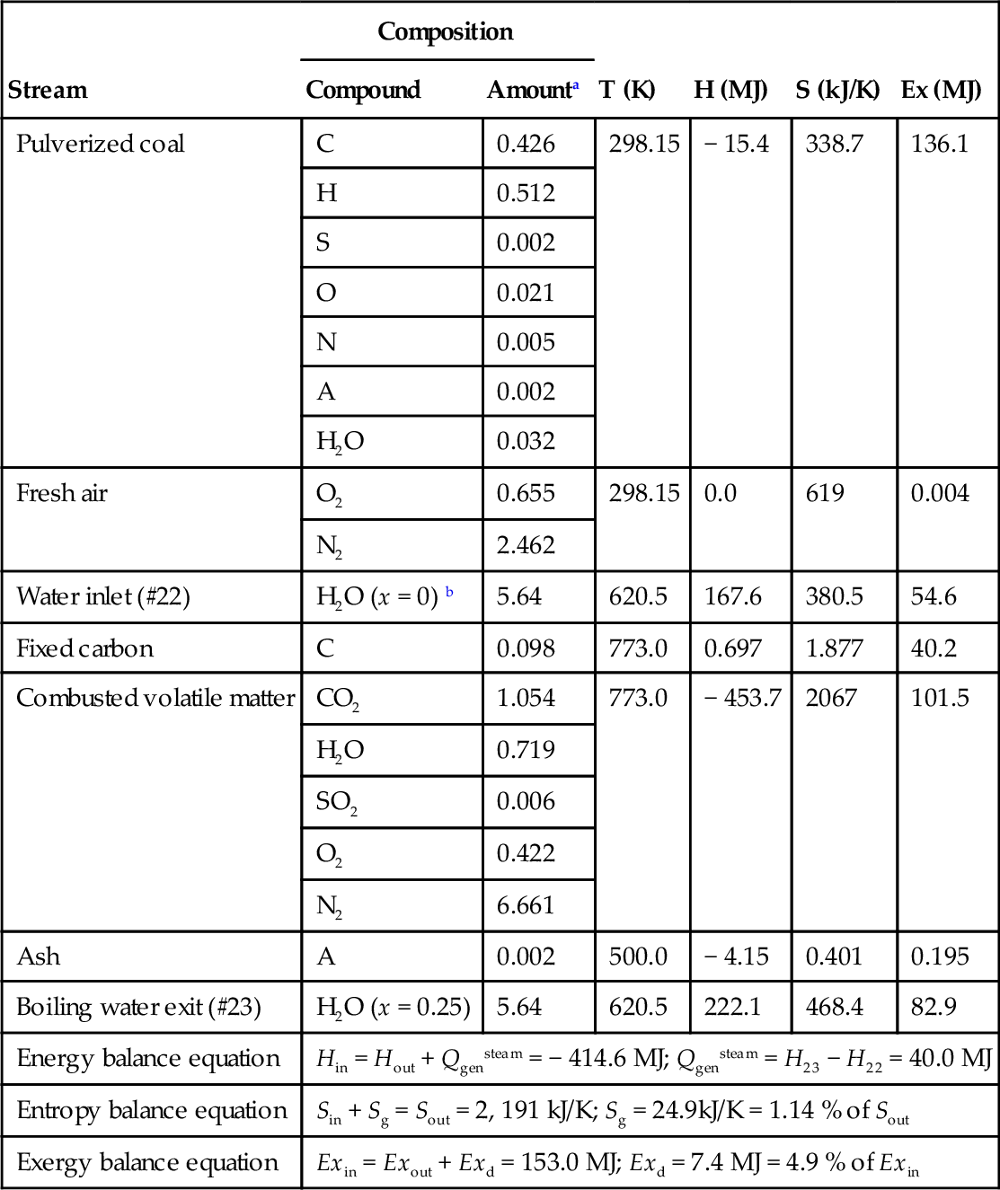
Table 5.19 gives the calculated stream concentrations, enthalpies, entropies, and chemical exergies for the first phase of the combustion process. For 1 kmol of coal supplied to the combustion process 5.64 kmol of water is circulated in the calandria tubes. Water boils partially up to a quality of 25% in the lower part of the furnace. The combusted volatile matter consisting of CO₂, H₂O, SO₂, and N₂ reaches a temperature of 773 K at point A. The bottom ash leaves the furnace at 500 K. Based on the energy balance equation it results that the enthalpy transferred to boiling water in region 0–A of the furnace is 40 MJ/kmol of supplied coal. The generated entropy represents 1.14% of output entropy whereas the destroyed exergy is 4.9% of the exergy at the input. Table 5.20 gives the streams parameters and the balance equations for the fixed carbon combustion zone of the furnace.

Table 5.19

Stream Parameters and Balance Equations for Ignition Zone

Stream	Composition		T (K)	H (MJ)	S (kJ/K)	Ex (MJ)
Stream	Compound	Amount^a	T (K)	H (MJ)	S (kJ/K)	Ex (MJ)
Pulverized coal	C	0.426	298.15	− 15.4	338.7	136.1
	H	0.512
	S	0.002
	O	0.021
	N	0.005
	A	0.002
	H₂O	0.032
Fresh air	O₂	0.655	298.15	0.0	619	0.004
Fresh air	N₂	2.462	298.15	0.0	619	0.004
Water inlet (#22)	H₂O (x = 0) ^b	5.64	620.5	167.6	380.5	54.6
Fixed carbon	C	0.098	773.0	0.697	1.877	40.2
Combusted volatile matter	CO₂	1.054	773.0	− 453.7	2067	101.5
	H₂O	0.719
	SO₂	0.006
	O₂	0.422
	N₂	6.661
Ash	A	0.002	500.0	− 4.15	0.401	0.195
Boiling water exit (#23)	H₂O (x = 0.25)	5.64	620.5	222.1	468.4	82.9
Energy balance equation	H_in = H_out + Q_gen^steam = − 414.6 MJ; Q_gen^steam = H₂₃ − H₂₂ = 40.0 MJ
Entropy balance equation	S_in + S_g = S_out = 2, 191 kJ/K; S_g = 24.9kJ/K = 1.14 % of S_out
Exergy balance equation	Ex_in = Ex_out + Ex_d = 153.0 MJ; Ex_d = 7.4 MJ = 4.9 % of Ex_in

t0100

^a Given in kmol component per kmol coal (as-received basis).

^b Formation enthalpy, formation entropy, and chemical exergy not included.

Table 5.20

Streams Parameters and Balance Equations for Carbon Combustion Zone

Stream	Composition		T (K)	H (MJ)	S (kJ/K)	Ex (MJ)
Stream	Compound	Amount^a	T (K)	H (MJ)	S (kJ/K)	Ex (MJ)
Boiling water outlet (#24)^b	H₂O (q = 0.35)	5.64	620.5	234.8	488.9	89.5
Combustion gases in B	CO₂	1.152	1073	− 467.9	2167	136.5
	H₂O	0.778
	SO₂	0.006
	O₂	0.295
	N₂	6.661
Energy balance equation	H_in = H_out + Q_gen^steam = − 454.6 MJ; Q_gen^steam = H₂₄ − H₂₃ = 13.3 MJ
Entropy balance equation	S_in + S_g = S_out = 2, 218 kJ/K; S_g = 26.8kJ/K = 1.23 % of S_out
Exergy balance equation	Ex_in = Ex_out + Ex_d = 145.5 MJ; Ex_d = 8.0 MJ = 5.5 % of Ex_in

t0105

Note: balances are given per unit of kmol of coal. The input streams are outputs of previous unit (Table 5.16).

^a kmol component per kmol coal.

^b Formation enthalpy, entropy, and chemical exergy not included for water.

From the table it results that in the calandria tubes of region A–B steam augments its vapor quality from 0.25 to 0.35. The heat input to steam is 13.3 MJ/kmol of coal fed; the entropy generation represents 1.23% of entropy in B while exergy destruction is 5.5% of exergy input in A. The vapor quality of steam at its return to the calandria drums in state 25 (Figure 5.26) is 75%.

The flue gas parameters in the non-combustion zone of the furnace comprising states C, D, E, and F (Figure 5.25) can be observed in Table 5.21. From this table it results that the exergy destruction at the superheater is 7.53 MJ/kmol of coal, whereas exergy destruction of the reheater is 2.18MJ/kmol. The exergy destruction of the economizer is reported as 2.38 MJ/kmol of coal.

Table 5.21

Stream Parameters and Irreversibilities for Furnace’s Non-Combustion Zones

Stream	T (K)	H (MJ)	S (kJ/K)	Ex (MJ)	Irreversibilities
Stream	T (K)	H (MJ)	S (kJ/K)	Ex (MJ)	Component	S_g (kJ/K)	Ex_d (MJ)
C	644	− 504.3	1932	76.3	Superheater	25.2	7.53
C	644	− 504.3	1932	76.3	Reheater	7.33	2.18
D	630	− 507.9	1926	74.4	Calandria boiler	0.15	0.05
E	473	− 550.1	1784	38.4	Economizer	8.00	2.38
F^a	473	220	713.6	15.4	Total	40.7	12.13

t0110

Note: the values of enthalpies, entropies, and exergies are given for 1 kmol of coal combusted.

^a Flue gas recirculation ratio: 0.6.

The balance equations are written for all components of the plant. A system of algebraic equations is formed which can be solved for thermodynamic parameters (temperature, pressure, enthalpy, entropy, exergy) at each state point. Values for the isentropic efficiency of the pumps and turbines must be assumed.

The imposed known parameters for modeling are the water condensation temperature at the condenser inlet and outlet, temperature of coal at feed (taken as T₀), boiling temperature (T₈), and superheating (T₉) and reheating (T₁₀) temperatures. Furthermore, the minimum temperature difference for heat exchangers is taken as ~10 K.

With these assumptions the algebraic equation system is closed and can be solved. Once thermodynamic state points are determined the irreversibilities in the form of entropy generation and exergy destruction are determined for each system component.

The system components are grouped into four major subsystems: furnace, turbines, condenser, and feedwater heating system. The results for each thermodynamic state are given in Table 5.22. The exergy destruction for each of the subsystems is shown graphically in Figure 5.30. The maximum exergy destruction is in the furnace, followed by the turbines. The HPT destroys 8.2% exergy, whereas the LPT destroys 31.7%.

Table 5.22

Working Fluid Stream Parameters (Example 5.7)

Stream	n	P	T	H	S	Ex	Stream	n	P	T	H	S	Ex
0^a	1	298.15	0.101	0.002	6.6	-0.082	13	0.4787	115.9	377	22,238	60.68	4187
1	3.84	4.246	303.2	8695	30.2	5.264	14	0.4787	115.9	377	3753	11.64	321.6
2	3.84	260.6	303.2	8716	30.21	23.13	15	0.4787	4.246	303.2	3753	12.57	44.68
3	3.84	260.6	367	27,200	85.54	2011	16	0.2577	260.6	402	12,496	32.37	2867
4	4.229	260.6	402	41,248	123.6	4745	17	1.752	551.1	428.7	83,845	207.2	22,223
5	4.229	16,000	404.1	42,750	124.2	6081	18	1.62	551.1	428.7	77,564	191.6	20,558
6	4.229	16,000	418.7	47,479	135.7	7383	19	0.1312	551.1	428.7	6281	15.52	1665
7	4.229	16,000	620.5	125,678	285.4	40,948	20	0.1312	551.1	428.7	1552	4.488	224.4
8	4.229	16,000	620.5	196,597	399.6	77,792	21	0.1312	260.6	402	1552	4.511	217.5
9	4.229	16,000	773.1	251,108	480.1	108,298	22	5.639	16,000	620.5	167,571	380.5	54,597
10	2.478	5530	620.5	136,008	284.5	51,394	23	5.639	16,000	620.5	222,106	468.4	82,930
11	2.478	5530	773.1	152,999	309	60,862	24	5.639	16,000	620.5	234,847	488.9	89,550
12	3.362	4.246	303.2	136,627	452	2133	25	5.639	16,000	620.5	238,490	494.8	91,442

t0115

n, number of moles (kmol/kmol coal); P, pressure (kPa); T, temperature (K); H, enthalpy (kJ/kmol coal); S, enthalpy (kJ/K for 1 kmol coal); Ex, exergy (kJ/kmol coal).

^a Reference state.

f05-30-9780123838605 — Figure 5.30 Exergy destructions and efficiencies of the studied coal-fired Rankine plant.

Figure 5.31 illustrates graphically the amounts of exergy destruction for each of the components of the furnace: calandria boiler (segments 0–A, A–B, C–D), superheater, reheater, and economizer. The subsystem destroys 19 MJ/kmol of coal (or 45.5% of input exergy). Proportionally, the superheater destroys the most exergy among the furnace components at 39.6%, followed by the first calandria segment (0–A) with 30.2% and the reheater with 11.5%.

f05-31-9780123838605 — Figure 5.31 Exergy destruction in the furnace.

A similar pie chart is presented in Figure 5.32 to show the exergy destruction of the components of the feedwater heating subsystem. Among the seven components (low-pressure feedwater heater, OFW, throttling valve 14, HPP, high-pressure feedwater heater, throttling valve 2, and LPP) the most exergy destruction (66.6%) happens in the low-pressure feedwater heater.

f05-32-9780123838605 — Figure 5.32 Exergy destruction in feedwater heating subsystem.

The energy and exergy efficiencies of the overall system result from Figure 4.24 and are 40.3% (energy) and 58.9% (exergy). Also the specific emissions of CO₂ and SO₂ can be calculated from Equation (5.15). Accordingly, $c = 0.426$ $c = 0.426$ moles of CO₂ are generated for mole of coal combusted; moreover, $s = 0.002$ $s = 0.002$ moles of SO₂ are produced for one mole of coal combusted. There is 756 g CO₂/kWh net power and 5.04 g SO₂/kWh net power. Figure 5.33 indicates the molar composition of flue gas as well as the specific CO₂ and SO₂ emissions.

f05-33-9780123838605 — Figure 5.33 Molar composition of flue gases and specific CO₂, SO₂ emissions.

5.2.6 Organic Rankine Cycles

Unlike the more common steam Rankine cycles, an organic working fluid is used in the ORCs. Local and small-scale power generation as well as renewable energy systems and low-grade heat recovery systems are the best applications for ORC technology. Some examples of low-temperature heat sources from renewable sources are solar radiation, biomass combustion systems, heat recovery systems from engine exhaust gases, geothermal energy, and ocean thermal energy.

ORC technology has received increased attention in the last decades. The manufacturers of ORC provide a wide range of solutions, based on the temperature level and sources. Table 5.23 gives a list of some existing ORC manufacturers and briefly describes their technology.

Table 5.23

List of some ORC Manufacturers and Technology Descriptions

Manufacturer	Power range	Heat source temperature	Technology description	Applications
ORMAT, US	200 KW–72 MW	150°–300 °C	Fluid : n-pentane	Geothermal, WHR, solar
Turboden, Italy	200 KW–2 MW	100°–300°C	Fluids: OMTS, Solkatherm Axial turbines	Geothermal, CHP
Adoratec, Germany	350 KW–1600 KW	300 °C	Fluid : OMTS	CHP
GMK, Germany	50 K–2 MW	120°–350 °C	Fluid: GL160 (GMK proprietary) 3000 rpm multistage axial turbines	Geothermal, CHP, WHR
Koehler-Ziegler, Germany	70–200 KW	150–270 °C	Fluid: Hydrocarbons, screw expander	CHP
UTC, US	280 KW	> 93 °C	N/A	Geothermal, WHR
Cryostar	N/A	100–400 °C	Fluids: R245fa, R134a Radial inflow turbine	WHR Geothermal
Freepower, UK	6 KW–120 KW	180–225 °C	N/A	WHR
Tri-o-gen, NL	160 KW	> 350 °C	Turbo-expander	WHR
Tri-o-gen, NL	50 KW	> 93 °C	Twin screw expander	WHR
Infinity turbine	250 KW	> 80 °C	Fluid: R134a Radial turbo expander	WHR

t0120

WHR, waste heat recovery; CHP, combined heating and power.

Working fluid characteristics have great influence in determining the cycle configuration. Selection of the working fluid must be done in compliance with the ORC application, which is influenced by the type of heat source, level of temperature, modes of heat transfer, and scale of the application. Pure fluids and fluid mixtures can both be considered. Also, the retrograde characteristic of the working fluid plays a crucial role in determining the cycle configuration. For example, if a retrograde fluid is used, then the expansion of saturated vapor occurs in the superheated region. This is due to the fact that the slope of the vapor saturation curve on a T–s diagram for retrograde fluids is always positive (e.g., toluene). On the other hand, if the fluid is regular then the expansion of saturated vapor occurs in the two-phase region. The slope of the vapor saturation curve of regular fluids is negative in the T–s diagram (e.g., R134a).

One important feature related to organic working fluid refers to the fact that a large pressure ratio over the turbine can be obtained for relatively small pressure differences. For example, with the organic fluid R123 the ORC operates at a boiling pressure of 5.87 bar and a condensation pressure of 0.85 bar. The pressure ratio is thus 6.9 and the pressure difference is 5.02 bar. This point signifies the advantage of using organic fluids as the working fluid in Rankine cycles. The most important fluid properties for organic working fluid selection are:

• Thermodynamic and physical properties such as density, boiling enthalpy, liquid heat capacity, viscosity, thermal conductivity, melting point temperature, normal boiling point, boiling latent heat (must be high), critical temperature, critical pressure, retrograde or regular behavior, and zeotropic or azeotropic characteristic in the case of mixtures.

• Environmental impact and safety factors such as ozone depletion potential (ODP), global warming potential (GWP), atmospheric lifetime (e.g., R11 45 years, R152 0.6 years), toxicity, flammability.

• Availability, stability at high temperature, and cost effectiveness.

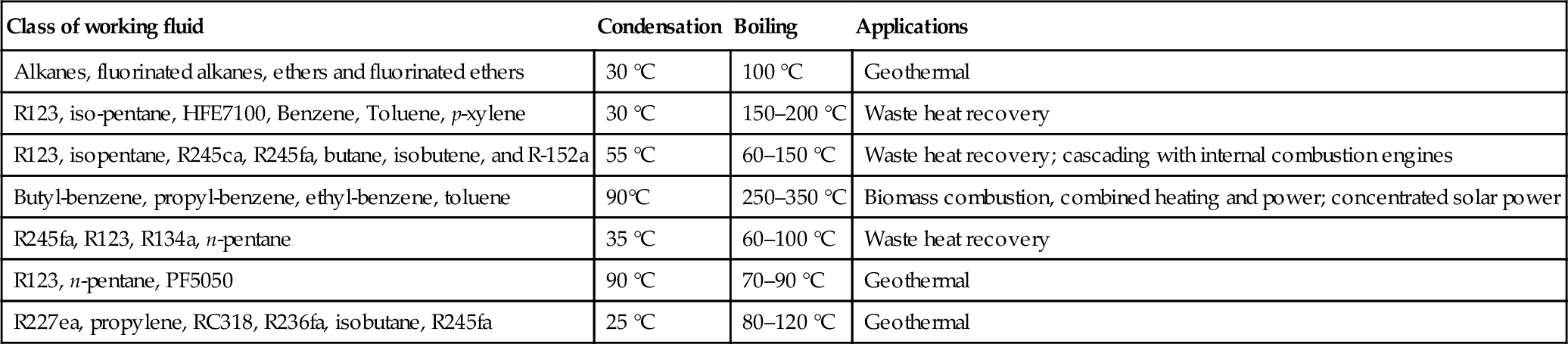
Table 5.24 gives the main categories of working fluids for ORCs and the typical applications for each category. Some proposed working fluids are propylene, propane, R227ea, R236fa, RC318, cyclohexane, R245fa, R141b, R365mfc, R11, R113, R114, toluene, fluorinol (CF₃CH₂OH), R41, R123, R245ca, isobutene, propane–ethane, and siloxanes (MM, MD4M, D4, D5). Table 5.24 lists the working fluids in order of their molecular masses and gives some main parameters, namely normal boiling point, critical pressure and temperature, ODP, and GWP.

Table 5.24

Classes of Working Fluids for ORC and Typical ORC Applications

Class of working fluid	Condensation	Boiling	Applications
Alkanes, fluorinated alkanes, ethers and fluorinated ethers	30 °C	100 °C	Geothermal
R123, iso-pentane, HFE7100, Benzene, Toluene, p-xylene	30 °C	150–200 °C	Waste heat recovery
R123, isopentane, R245ca, R245fa, butane, isobutene, and R-152a	55 °C	60–150 °C	Waste heat recovery; cascading with internal combustion engines
Butyl-benzene, propyl-benzene, ethyl-benzene, toluene	90°C	250–350 °C	Biomass combustion, combined heating and power; concentrated solar power
R245fa, R123, R134a, n-pentane	35 °C	60–100 °C	Waste heat recovery
R123, n-pentane, PF5050	90 °C	70–90 °C	Geothermal
R227ea, propylene, RC318, R236fa, isobutane, R245fa	25 °C	80–120 °C	Geothermal

t0125

Both turbo-expanders and positive displacement expanders are considered prime movers for ORCs. The choice depends on the scale of the application, the working fluid, pressure differentials, and pressure and volume ratios. For large-scale applications turbo-expanders will be the preferred choice because of their higher efficiency. At lower-scale applications, when pressure drop across the prime mover must be high, the preferred choice is a positive displacement expander because it has contact seals which reduce the bypass leakages. When pressure difference per stage is high, turbo-expanders (turbines) have bypass leakage flow at blade tips which is accentuated for small-scale applications.

There are many configurations of the ORC which differ from the typical reheat-regenerative steam cycle configuration that normally uses steam extraction. For example, in ORC with retrograde fluid it is possible to use a counter-current heat exchanger as a regenerator. In addition, ORC with retrograde fluids can operate without superheating, which makes them better suited for applications that involve heat recovery or solar energy. Other configurations are the reheat-regeneration cycle and supercritical cycle.

An ORC of simple configuration is shown in Figure 5.34. The cycle operates with the organic fluid R134a and is heated with a hot fluid. This cycle configuration can be applied for waste heat recovery when the heat source is low grade. Notice that superheating is not required because the moisture at the end of the expansion process is very low when saturated vapors are expanded (Table 5.25).

f05-34-9780123838605 — Figure 5.34 Simple four-component ORC with R134a for low-grade waste heat recovery.

Table 5.25

Working Fluids Commonly Used in ORC

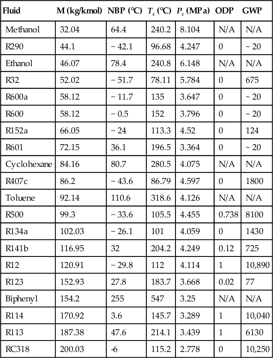
Fluid	M (kg/kmol)	NBP (°C)	T_c (°C)	P_c (MPa)	ODP	GWP
Methanol	32.04	64.4	240.2	8.104	N/A	N/A
R290	44.1	− 42.1	96.68	4.247	0	~ 20
Ethanol	46.07	78.4	240.8	6.148	N/A	N/A
R32	52.02	− 51.7	78.11	5.784	0	675
R600a	58.12	− 11.7	135	3.647	0	~ 20
R600	58.12	− 0.5	152	3.796	0	~ 20
R152a	66.05	− 24	113.3	4.52	0	124
R601	72.15	36.1	196.5	3.364	0	~ 20
Cyclohexane	84.16	80.7	280.5	4.075	N/A	N/A
R407c	86.2	− 43.6	86.79	4.597	0	1800
Toluene	92.14	110.6	318.6	4.126	N/A	N/A
R500	99.3	− 33.6	105.5	4.455	0.738	8100
R134a	102.03	− 26.1	101	4.059	0	1430
R141b	116.95	32	204.2	4.249	0.12	725
R12	120.91	− 29.8	112	4.114	1	10,890
R123	152.93	27.8	183.7	3.668	0.02	77
Biphenyl	154.2	255	547	3.25	N/A	N/A
R114	170.92	3.6	145.7	3.289	1	10,040
R113	187.38	47.6	214.1	3.439	1	6130
RC318	200.03	-6	115.2	2.778	0	10,250

t0130

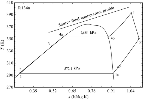
The regenerative schemes for ORC do not require (in general) vapor extraction (as in the case of steam cycles). Rather an additional heat exchanger is inserted between the turbine exit and the pump exit, which allows for a transfer of heat between the hotter working fluid at the turbine exhaust and the colder liquid at the pump discharge. The configuration of a regenerative ORC is presented in Figure 5.35. An example of ORC with regeneration that uses R134a as working fluid is presented in Figure 5.36. In this cycle, boiling occurs at 353 K; it starts with saturated liquid in state 4a and reaches saturated vapor in state 4b (pressure drop is neglected). In the condenser, there is a de-superheating process according to line 6–1a, where 1a represents saturated vapor (see Figure 5.36). Further, the condensation process continues until reaching saturated liquid in state 1.

f05-35-9780123838605 — Figure 5.35 Regenerative ORC configuration.

f05-36-9780123838605 — Figure 5.36 Regenerative ORC with R134a for low-grade heat sources.

The exergy destruction in the regenerator is accounted for with the help of regenerator effectiveness. This parameter is defined based on the sketch in Figure 5.37, which illustrates a regenerator in the form of a heat exchanger that facilitates a heat transfer process between a hotter stream and a colder stream. Both streams exchange sensible heat. The effectiveness is defined by the ratio between the heat transfer rate that ideally can be extracted from the hotter stream ( ${\dot{Q}}_{ideal}$ ${\dot{Q}}_{ideal}$ ) and the heat which is actually received by the colder stream ( $\dot{Q} = {\dot{m}}_{colder} (h_{4} - h_{3}))$ $\dot{Q} = {\dot{m}}_{colder} (h_{4} - h_{3}))$ . Note that the ideal, maximum heat rate that the hotter fluid can transfer occurs when T₂ = T₃ (see Figure 5.37); therefore the ideal maximum heat transfer in the regenerator occurs when h₂ = h₂(T₃) and is given by ${\dot{Q}}_{ideal} = {\dot{m}}_{hotter} (h_{1} - h_{2} (T_{3}))$ ${\dot{Q}}_{ideal} = {\dot{m}}_{hotter} (h_{1} - h_{2} (T_{3}))$ . According to this definition, the regenerator effectiveness is

$ɛ_{reg} = \frac{\dot{Q}}{{\dot{Q}}_{ideal}} = \frac{{\dot{m}}_{colder} (h_{4} - h_{3})}{{\dot{m}}_{hotter} (h_{1} - h_{2} (T_{3}))}$ $ɛ_{reg} = \frac{\dot{Q}}{{\dot{Q}}_{ideal}} = \frac{{\dot{m}}_{colder} (h_{4} - h_{3})}{{\dot{m}}_{hotter} (h_{1} - h_{2} (T_{3}))}$

si331_e (5.23)

f05-37-9780123838605 — Figure 5.37 Sketch for the definition of regenerator effectiveness.

An interesting type of regenerative ORC is that using retrograde working fluids where saturated vapor is fed into the turbine while the expanded fluid is in superheated state. An example of such a cycle is shown in Figure 5.38, with toluene as the working fluid. As seen, the boiling temperature is 573 K and the boiling pressure is 1665 kPa. For a condensation at 303 K the saturation pressure is 2.911 kP (vacuum). Therefore the pressure ratio over the turbine is 395; at the same time the volumetric expansion ratio is 285. Figure 5.38 is suggested the temperature profile at the source when a hot fluid which exchanges sensible heat is used as the heat source (e.g., hot combustion gases, high-temperature geothermal brine, etc.).

f05-38-9780123838605 — Figure 5.38 ORC with a retrograde working fluid (toluene) and expansion of saturated vapor.

An emerging type of ORC is the supercritical cycle. This cycle works generally based on a scheme with regeneration such as that presented in Figure 5.35. In supercritical cycles the working fluid is pressurized to supercritical pressure and heated. As the pressure is supercritical, there is no boiling during heating. Rather, when the temperature becomes superior to critical point the working fluid enters into a supercritical state where the thermodynamic properties are neither of a liquid nor of a gas but a combination of these. Given that there is no boiling, the typical pinch point problem that occurs in vapor generators for Rankine cycles is minimized. Therefore, a gain on exergy efficiency can be obtained with respect to cycles with boiling. However, due to the high pressures associated with supercritical cycles, one must exercise care when selecting a working fluid.

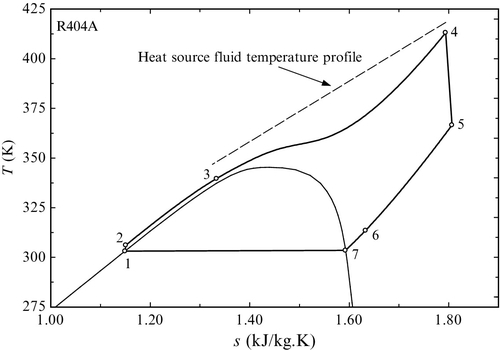
An example of a supercritical ORC operating with R404A working fluid (which is a blend of refrigerants) is shown in Figure 5.39. The high pressure in this cycle is 44.82 bar while the low pressure is 14.28 bar, making a pressure ratio of 3.1, which is applicable to positive displacement expanders. The temperature profiles match very well, proving that there is reduced exergy destruction in a supercritical ORC. In the regenerative heat exchanger a pinch point appears due to the nonlinear temperature profile of the supercritical fluid.

f05-39-9780123838605 — Figure 5.39 Supercritical-regenerative ORC with R404a (refrigerants blend).

Example 5.8

In this example the thermodynamic analysis of a regenerative cycle with the retrograde fluid toluene is demonstrated. The cycle configuration is according to Figure 5.35. Assume that the boiling temperature is 525 K, condensation is at 305 K cooled with water, the isentropic efficiency of the pump is 0.8, and isentropic efficiency of the turbine is 0.9. The heat source is a hot flue gas of 650 K that is assumed as ideal gas air. The minimum temperature difference in the heat exchangers is 10 K and the log mean temperature difference (LMTD) at the condenser is 18 K. We will determine the efficiencies, the exergy destructions, and the effectiveness of the regenerator and the mass flow rates for 100 kW power generated.

The balance equations in conjunction with the algebraic equations for pump and turbine isentropic efficiency and the temperature assumptions form a closed system that can be solved to determine the thermodynamic parameters for each state point. Table 5.26 gives the assumptions and balance equations for each of the cycle components.

Table 5.26

Balance Equations for Example 5.8

Component	Process	Assumptions	Balance equations
Pump	1–2	h_2s − h₁ = η_S,p(h₂ − h₁) with η_S,p = 0.8 adiabatic; x₁ = 0	MBE: ${\dot{m}}_{1} = {\dot{m}}_{2} = \dot{m}$ ${\dot{m}}_{1} = {\dot{m}}_{2} = \dot{m}$ EBE: ${\dot{m}}_{1} h_{1} + \dot{W_{p}} = {\dot{m}}_{2} h_{2}$ ${\dot{m}}_{1} h_{1} + \dot{W_{p}} = {\dot{m}}_{2} h_{2}$ EnBE: ${\dot{m}}_{1} s_{1} + {\dot{S}}_{g} = {\dot{m}}_{2} s_{2}$ ${\dot{m}}_{1} s_{1} + {\dot{S}}_{g} = {\dot{m}}_{2} s_{2}$ ExBE: ${\dot{m}}_{1} e x_{1} + \dot{W_{p}} = {\dot{m}}_{2} e x_{2}$ ${\dot{m}}_{1} e x_{1} + \dot{W_{p}} = {\dot{m}}_{2} e x_{2}$
Regenerator	2–3 and 5–6	T₆ = T₂ − 10 $ɛ_{reg} = \frac{h_{3} - h_{2}}{h_{5} - h_{(P_{5}, T_{2})}}$ $ɛ_{reg} = \frac{h_{3} - h_{2}}{h_{5} - h_{(P_{5}, T_{2})}}$ , adiabatic	MBE: ${\dot{m}}_{2} = {\dot{m}}_{3} = {\dot{m}}_{5} = {\dot{m}}_{6} = \dot{m}$ ${\dot{m}}_{2} = {\dot{m}}_{3} = {\dot{m}}_{5} = {\dot{m}}_{6} = \dot{m}$ EBE: ${\dot{m}}_{2} h_{2} + {\dot{m}}_{5} h_{5} = {\dot{m}}_{3} h_{3} + {\dot{m}}_{6} h_{6}$ ${\dot{m}}_{2} h_{2} + {\dot{m}}_{5} h_{5} = {\dot{m}}_{3} h_{3} + {\dot{m}}_{6} h_{6}$ EnBE: ${\dot{m}}_{2} s_{2} + {\dot{m}}_{5} s_{5} + {\dot{S}}_{g} = {\dot{m}}_{3} s_{3} + {\dot{m}}_{6} s_{6}$ ${\dot{m}}_{2} s_{2} + {\dot{m}}_{5} s_{5} + {\dot{S}}_{g} = {\dot{m}}_{3} s_{3} + {\dot{m}}_{6} s_{6}$ ExBE: ${\dot{m}}_{2} e x_{2} + {\dot{m}}_{5} e x_{5} = {\dot{m}}_{3} e x_{3} + {\dot{m}}_{6} e x_{6} + \dot{E} x_{d}$ ${\dot{m}}_{2} e x_{2} + {\dot{m}}_{5} e x_{5} = {\dot{m}}_{3} e x_{3} + {\dot{m}}_{6} e x_{6} + \dot{E} x_{d}$
Vapor generator	3–4	T_so,1 = T₄ + 10 T_so,pinch = T_4a + 10, adiabatic, isobaric	MBE: ${\dot{m}}_{3} = {\dot{m}}_{4} = \dot{m}; {\dot{m}}_{so, 1} = {\dot{m}}_{so, 2} = {\dot{m}}_{so}$ ${\dot{m}}_{3} = {\dot{m}}_{4} = \dot{m}; {\dot{m}}_{so, 1} = {\dot{m}}_{so, 2} = {\dot{m}}_{so}$ EBE: ${\dot{m}}_{3} h_{3} + {\dot{m}}_{so, 1} h_{so, 1} = {\dot{m}}_{4} h_{4} + {\dot{m}}_{so, 2} h_{so, 2}$ ${\dot{m}}_{3} h_{3} + {\dot{m}}_{so, 1} h_{so, 1} = {\dot{m}}_{4} h_{4} + {\dot{m}}_{so, 2} h_{so, 2}$ EnBE: ${\dot{m}}_{3} s_{3} + {\dot{m}}_{so, 1} s_{so, 1} + {\dot{S}}_{g} = {\dot{m}}_{4} s_{4} + {\dot{m}}_{so, 2} s_{so, 2}$ ${\dot{m}}_{3} s_{3} + {\dot{m}}_{so, 1} s_{so, 1} + {\dot{S}}_{g} = {\dot{m}}_{4} s_{4} + {\dot{m}}_{so, 2} s_{so, 2}$ ExBE: ${\dot{m}}_{3} e x_{3} + {\dot{m}}_{so, 1} e x_{so, 1} = {\dot{m}}_{4} e x_{4} + {\dot{m}}_{so, 2} e x_{so, 2} + \dot{E} x_{d}$ ${\dot{m}}_{3} e x_{3} + {\dot{m}}_{so, 1} e x_{so, 1} = {\dot{m}}_{4} e x_{4} + {\dot{m}}_{so, 2} e x_{so, 2} + \dot{E} x_{d}$
Turbine	4–5	h₄ − h₅ = η_S,t(h₄ − h_5s) with η_S,t = 0.9, adiabatic	MBE: ${\dot{m}}_{4} = {\dot{m}}_{5} = \dot{m}$ ${\dot{m}}_{4} = {\dot{m}}_{5} = \dot{m}$ EBE: ${\dot{m}}_{4} h_{4} = {\dot{m}}_{5} h_{5} + \dot{W_{t}}$ ${\dot{m}}_{4} h_{4} = {\dot{m}}_{5} h_{5} + \dot{W_{t}}$ EnBE: ${\dot{m}}_{4} s_{4} + {\dot{S}}_{g} = {\dot{m}}_{5} s_{5}$ ${\dot{m}}_{4} s_{4} + {\dot{S}}_{g} = {\dot{m}}_{5} s_{5}$ ExBE: ${\dot{m}}_{4} e x_{4} = {\dot{m}}_{5} e x_{5} + \dot{W_{t}} + \dot{E} x_{d}$ ${\dot{m}}_{4} e x_{4} = {\dot{m}}_{5} e x_{5} + \dot{W_{t}} + \dot{E} x_{d}$
Condenser	6–1	ΔT_pinch = T_1a − T_si = 10 K LMTD_si = 10 K, adiabatic, isobaric	MBE: ${\dot{m}}_{6} = {\dot{m}}_{1} = \dot{m}; {\dot{m}}_{si, 1} = {\dot{m}}_{si, 2} = {\dot{m}}_{si}$ ${\dot{m}}_{6} = {\dot{m}}_{1} = \dot{m}; {\dot{m}}_{si, 1} = {\dot{m}}_{si, 2} = {\dot{m}}_{si}$ EBE: ${\dot{m}}_{6} h_{6} + {\dot{m}}_{si, 1} h_{si, 1} = {\dot{m}}_{1} h_{1} + {\dot{m}}_{si, 2} h_{si, 2}$ ${\dot{m}}_{6} h_{6} + {\dot{m}}_{si, 1} h_{si, 1} = {\dot{m}}_{1} h_{1} + {\dot{m}}_{si, 2} h_{si, 2}$ EnBE: ${\dot{m}}_{6} s_{6} + {\dot{m}}_{si, 1} s_{si, 1} + {\dot{S}}_{g} = {\dot{m}}_{1} s_{1} + {\dot{m}}_{si, 2} s_{si, 2}$ ${\dot{m}}_{6} s_{6} + {\dot{m}}_{si, 1} s_{si, 1} + {\dot{S}}_{g} = {\dot{m}}_{1} s_{1} + {\dot{m}}_{si, 2} s_{si, 2}$ ExBE: ${\dot{m}}_{6} e x_{6} + {\dot{m}}_{si, 1} e x_{si, 1} = {\dot{m}}_{1} e x_{1} + {\dot{m}}_{si, 2} e x_{si, 2} + \dot{E} x_{d}$ ${\dot{m}}_{6} e x_{6} + {\dot{m}}_{si, 1} e x_{si, 1} = {\dot{m}}_{1} e x_{1} + {\dot{m}}_{si, 2} e x_{si, 2} + \dot{E} x_{d}$

t0135

The chemical exergies do not need to be considered because there is no chemical reaction. For the thermomechanical exergy calculation the standard reference state of T₀ = 298.15 K and P₀ = 101.325 kPa is considered. For toluene, which is always enclosed inside the heat engine circuits, the reference state is saturated liquid at T₀.

A pinch point calculation procedure must be applied for both the vapor generator and the condenser. In this respect, the requirement of a 10 K-minimum temperature difference is called. Hence, the temperature of the gas at source side must be superior by 10 K with respect to the working fluid temperature at state 4a, which corresponds to the pinch point. In addition we assume that the temperature difference between the source inlet temperature and the working fluid temperature at the turbine entrance is 10 K. Regarding the condenser, a temperature difference between the saturated vapor (state 1a) and the water coolant of 10 K is imposed (this corresponds to the pinch point). Further, the temperature of water at inlet must be iterated until LMTD at the condenser becomes 18 K. The LMTD must be calculated with ΔT₁ = T₁ − T_si,1 where T_si,1 is the water temperature at sink inlet and ΔT₂ = T₆ − T_si,2 where T_si,2 is the water temperature at sink outlet. The known equation for LMTD is: LMTD = (ΔT_max − ΔT_min)/ln(ΔT_max/ΔT_min) where ΔT_min = min(ΔT₁, ΔT₂) and ΔT_max = max(ΔT₁, ΔT₂).

The temperatures, pressures, and enthalpy, entropy, and exergy rates for each thermodynamic state of the cycle are given in Table 5.27. In the same table the rates of heat and work transfer and the rate of exergy destruction for each cycle component are also given. The energy efficiency of the cycle is 38% while the exergy efficiency of 50%. Based on 100 kW net power generation the mass flow rate of the working fluid must be 0.3786 kg/s.

Table 5.27

Thermodynamic State Points, Components, and Cycle Parameters for Example 5.8

State	T (K)	P (kPa)	$\dot{H}$ $\dot{H}$ (kW)	$\dot{S}$ $\dot{S}$ (kW/K)	$\dot{Ex}$ $\dot{Ex}$ (kW)	Component	$\dot{Q}$ $\dot{Q}$ (kW)	$\dot{W}$ $\dot{W}$ (kW)	$\dot{E} x_{d}$ $\dot{E} x_{d}$ (kW)
1	305	5.362	− 56.78	− 0.165	0.05225	Pump	N/A	0.96	0.188
2	305.7	1710	− 55.82	− 0.1644	0.8287	Regenerator	119.7	N/A	6.613
3	459.9	1710	63.84	0.1494	26.92	Vapor generator	263.3	N/A	8.668
4a	525	1710	126.4	0.2765	51.63	Turbine	N/A	100.96	6.615
4b	525	1710	216.2	0.4476	90.4	Condenser	163.3	N/A	7.187
4	650	1710	327.2	0.6371	144.9	Cycle parameters
5	513.3	5.362	226.2	0.6593	37.29	Energy efficiency		η = 38%
6	315.7	5.362	106.6	0.3703	3.804	Exergy efficiency		ψ = 50%
1a	305	5.362	101.7	0.3526	4.182	Mass flow rate	Working fluid	$\dot{m} = 0.3786$ $\dot{m} = 0.3786$ kg/s
1_so	660	101.3	1025	11.73	198		Source fluid	${\dot{m}}_{so} = 1.528$ ${\dot{m}}_{so} = 1.528$ kg/s
2_so	535	101.3	824.6	11.39	97.69		Sink fluid	${\dot{m}}_{si} = 6.159$ ${\dot{m}}_{si} = 6.159$ kg/s
1_si	288.9	101.3	406.1	1.443	− 24.24	Turbine	Pressure ratio	PR = 319
2_si	295	101.3	564.6	1.986	− 27.63		Expansion ratio	ER = 285

t0140

In Figure 5.40a the thermodynamic cycle is illustrated in the T–s diagram. On the same diagram the temperature profiles of the heat source and heat sink fluids are suggested. This illustrates the irreversibility due to the finite temperature difference for heat transfer at heat source and heat sink heat exchangers. The exergy destructions by the cycle components are represented in the chart in Figure 5.40b. As seen, the exergy destructions are well balanced among the cycle components, except for the pump, which destroys negligible exergy.

f05-40-9780123838605 — Figure 5.40 ORC with toluene for Example 5.8; (a) thermodynamic cycle, (b) exergy destruction percentages.

..................Content has been hidden....................

You can't read the all page of ebook, please click here login for view all page.

Table of Contents for Advanced Power Generation Systems

Create new playlist

Sign In

Sign Up

5.2.5 Steam Rankine Power Stations

5.2.5.1 Reheating-Regenerative Steam Rankine Cycle

5.2.5.2 Coal-Fired Power Stations

5.2.6 Organic Rankine Cycles

Table of Contents for
Advanced Power Generation Systems