This bonus chapter contains additional techniques that cover a wide range of topics. Although none of the techniques are mandatory for successful animation, they can strengthen your knowledge and allow you to be more flexible when solving lighting and texturing problems. Each section is numbered to correspond to the chapter most closely linked to the topic. For example, section 4.1 and 4.2 cover additional applications of the Ramp texture, which was initially discussed in Chapter 4.
You can create a custom wireframe render for a polygon surface with a Ramp texture. A simplified version of the scene illustrated by Figure A.1 is included as wireframe.ma on the CD in the Additional_Techniques scene folder.
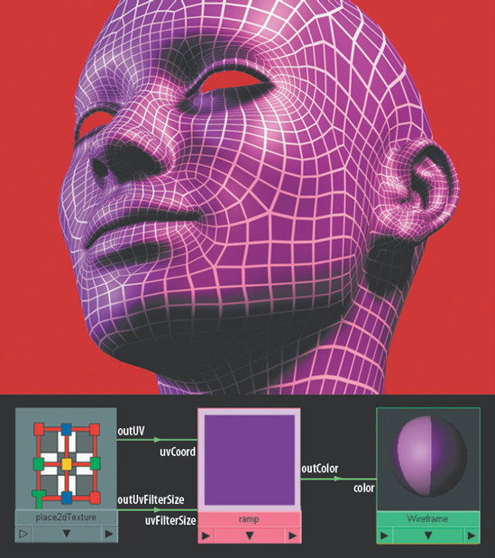
For this custom shading network to work, the polygons of the model must be unitized (whereby each polygon face takes up 100 percent of the UV texture space). This can be achieved by switching to the Polygons menu set and choosing Edit UVs > Unitize as the polygon surface is selected. Once unitized, each polygon face receives the complete Ramp texture. As for the Ramp colors, a light purple handle rests at the top with a dark purple handle just below it. Most important, the ramp Type attribute is set to Box Ramp and Interpolation is set to None.
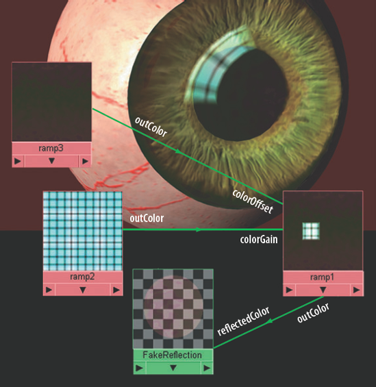
You can create the detailed reflection of a window in the cornea of an eye by using several Ramp textures. The scene in Figure A.2 is included as window.ma on the CD in the Additional_Techniques scene folder.
As discussed in Chapter 4, specular highlights are simply reflected light sources; hence, they are rarely the spherical shape provided by default Blinn, Phong, or Phong E materials.
In this example, the outColor of a ramp texture node (ramp1) is connected to the reflectedColor of a blinn material node (named FakeReflection). Reflected Color allows the appearance of a reflection without the need to raytrace. The texture mapped to Reflected Color is laid on top of the surface it's assigned to; the top right of the texture appears at the top-right of the surface UV texture space. The blinn material node is given a 100 percent white Transparency and assigned to the cornea geometry. The Type attribute of ramp1 is set to Box Ramp and the Interpolation is set to Linear. Two color handles are placed close together to create a slightly soft edge on the resulting small, white box. For ramp1's place2dTexture node, the Offset is set to 0.15, 0, which slides the entire ramp slightly to the left.
The outColor of a second ramp texture node (ramp2) is connected to the colorGain of ramp1. The Type attribute of ramp2 is set to Tartan and Interpolation is set to Linear. The color handles are adjusted to create a grid pattern appropriate for window panes. A pale blue is picked to emulate sky color. The place2dTexture node of ramp2 has a Repeat UV value of 2.8, 2.8, which shrinks the grid.
The outColor of a third ramp texture node (ramp3) is connected to the colorOffset of ramp1. The color handles are set to dark browns and yellows. Noise is set to 0.2 and Noise Frequency is set to 1. This creates a random pattern that appears in the areas not covered by the window. When ramp3 is mapped to the Color Offset, the blacks of ramp1 are given a subtle wash of color. Last, the Eccentricity of the blinn node is turned down to 0. This prevents the default specular highlight from appearing and interfering with the Reflected Color.
The Clamp utility is not limited to color values. For example, you can control the scale of a character bicep with a Clamp utility. The scene in Figure A.3 is included as bicep.ma on the CD in the Additional_Techniques scene folder. To view the custom network, follow these steps:
Open the Hypershade window and switch to the Utilities tab.
MMB-drag the clamp node into the work area.
With the clamp node selected, click the Input And Output Connections button. A portion of the network becomes visible.
Select the elbow and bicep transform nodes and click the Input And Output Connections button again. All the components of the network become visible.
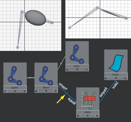
The rotateY of an elbow joint is connected to the inputR of a clamp node. In this case, the label for the connection reads "unitConversion." A unit conversion utility node is inserted automatically between the joint and clamp nodes when such a custom connection is made. This is due to the dissimilar units of measure employed by each node. The joint employs angular degree units and the clamp uses generic linear units. Although unit conversion nodes are not visible in the Hypershade in some situations, you can view them in the Hypergraph Connections window if Show > Show Auxiliary Nodes is selected from the Hypergraph menu. (For more information on the Unit Conversion utility, see Chapter 8.)
The outputR of the clamp node is connected to the scaleZ of a NURBS surface bicep transform node. To create such a connection between a utility node and a geometry transform node, you can MMB-drag a geometry transform node from the Hypergraph Hierarchy window into the Hypershade work area. The MinR of the clamp node is set to 0.1 and the MaxR is set to 2. When the elbow joint is rotated, it automatically scales the bicep. The scale of the bicep is kept between 0.1 and 2 by the clamp node. Although this setup can be created more accurately with an expression, it shows the flexibility of custom connections within the Hypershade.
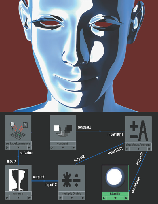
You can use the Surface Luminance utility to create stylized materials. For example, in Figure A.4 unique chrome is demonstrated. A simplified version of this scene is included as chrome.ma on the CD in the Additional_Techniques scene folder. A QuickTime movie is included as chrome.mov. To view the custom network, follow these steps:
Open the Hypershade window and switch to the Utilities tab.
MMB-drag the contrast node and surfaceLuminance node into the work area.
With both nodes selected, click the Input And Output Connections button. The network becomes visible.
In this network, the outValue of a surfaceLuminance node is connected to the inputX of a reverse node (see Chapter 8 for a description of the Reverse utility). The outputX of the reverse node is connected to the input1X of a multiplyDivide node. The outputX of the multiplyDivide is connected to the input1D[0] of a plusMinusAverage node. The output1D of the plusMinusAverage node is connected to the cosinePower of a phong material node named Chrome. This has the effect of artificially increasing the specular size of any part of the surface that receives more light.
Normally, the Phong's Cosine Power slider will not drop below 2. While many sliders can be readjusted to have a greater range (see "A Note on Sliders and Super-White" in Chapter 6), the Cosine Power attribute will not permit this—unless it carries a custom connection. As the Cosine Power value drops below the standard minimum threshold of 2, it causes the specular highlight to cover the entire lit side of the model. In addition, the highlight's core becomes unnaturally dark and the highlight's edge becomes more intense. For the shading network illustrated in Figure A.4, the following math occurs:
cosinePower = ((1 - outValue) * 2) - 2
If the surfaceLuminance node's outValue is 1 (maximum amount of light), then the cosinePower attribute becomes −2. If the surfaceLuminance node's outValue is 0 (no light received), then the cosinePower becomes 0. In other words, wherever the surface is bright, the phong node receives an artificially negative cosinePower. Wherever the surface is dark, the phong node receives a cosinePower closer to the normal minimum.
In this shading network, the contrastX of a contrast utility node is connected to the input1D[1] of the plusMinusAverage node. The contrast node simply serves as a generic placeholder, which is able to provide the −2 portion of the formula. The Operation of the plusMinusAverage node is set to Sum. The reverse node provides the (1 - outValue) portion of the formula. The multiplyDivide node provides the * 2 portion of the formula.
The hue of an iridescent surface changes with the angle of view. In the real world, this is caused by surfaces composed of multiple, semitransparent layers that create interference patterns in reflected light. This effect is commonly seen on butterfly wings, insect shells, fish scales, and some blown glass. Nevertheless, it's possible to emulate this look with a Sampler Info utility by using its Facing Ratio attribute. A simplified version of the scene in Figure A.5 is included as iridescence.ma on the CD in the Additional_Techniques scene folder. A QuickTime movie is included as iridescence.mov. To view the custom network, follow these steps:
Open the Hypershade window and switch to the Utilities tab.
MMB-drag the clamp node into the work area.
With the clamp node selected, click the Input And Output Connections button. The network becomes visible.
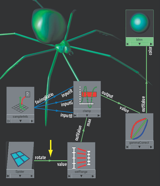
In Figure A.5, the facingRatio of a samplerInfo node is connected to the inputR, inputG, and inputB of a clamp node. The clamp node's Min attribute is set to 0, 0.3, 0.7, which biases the values from the samplerInfo node toward the green and blue channel. The output of the clamp node is connected to the value of a gammaCorrect node. The Gamma attribute of the gammaCorrect node is set to 0.3, 0.6, 0.2, which further adjusts the values derived from the samplerInfo node. The gammaCorrect node's bias toward the green channel gives the surface its green cast. However, the inclusion of the spider's transform node and a setRange node in the network causes deep blue, sky blue, lavender, and red bands to appear on the surface. Last, the outValue of the gammaCorrect node is connected to the color of a blinn material node, which is assigned to a polygon spider.
The clamp node provides the following logic:
IffacingRatio= 0, then RGB = 0, 0.3, 0.7 (deep blue) IffacingRatio= 0.5, then RGB = 0.5, 0.5, 0.7 (lavender) IffacingRatio= 1, then RGB = 0.5, 0.65, 0.85 (sky blue)
The max attribute used by the clamp node is actually provided by the geometry. When the spider's rotate values are 0, 0, 0 and the facingRatio is 1, the max value remains 0.5, 0.65, 0.85. When the rotation is changed, the max value shifts. This is accomplished by connecting the rotate attribute of the spider transform node to the value of a setRange node. (See Chapter 8 for a description of the Set Range utility.) The outValue of the setRange node is connected to the max of the clamp node. The setRange node converts the spider's rotational range to a smaller one usable by the clamp node. The Old Min attribute of the setRange node is set to −360, −360, −360. The Old Max attribute is set to 360, 360, 360. The −360 to 360 range is converted into a new range that runs somewhere between 0 and 1. Since the Min attribute of the setRange node is set to 0, 0.3, 0.7, each color channel of the clamp node's Max attribute receives a unique range. For example, the following occurs when the spider has two different rotations:
If spiderRotate= 0, 0, 360, then clampMax= 0.5, 0.65, 1 If spiderRotate= 180, 180, 180, then clampMax= 0.75, 0.825, 0.925
In the end, the more the spider rotates in X, the redder it gets at its core. The more the spider rotates in Y, the greener it gets at its core. The more it rotates in Z, the bluer it gets at its core. The edge colors do not shift away from dark blue since the facingRatio values remain low and always force the clamp node to output values close to the Min attribute values, which are 0, 0.3, 0.7.
Translucence is the ability of a material to diffuse light below its surface. Human and bare animal skin does this naturally. In sunlight, the effect is most commonly seen along the edge of the ear. Although many Maya materials contain the Translucence attribute, the attribute can be difficult to adjust in some situations (see Chapter 4 for more information). Therefore, creating a simulated translucence is sometimes warranted. This can be achieved by employing Surface Luminance and Light Info utilities. The scene in Figure A.6 is included as translucence.ma on the CD in the Additional_Techniques scene folder. A QuickTime movie is included as translucence.mov.
In Figure A.6, a custom shading network is divided into three sections. Although it is not necessary to use all three sections when creating a skin-shading network, each section demonstrates potentially useful techniques.
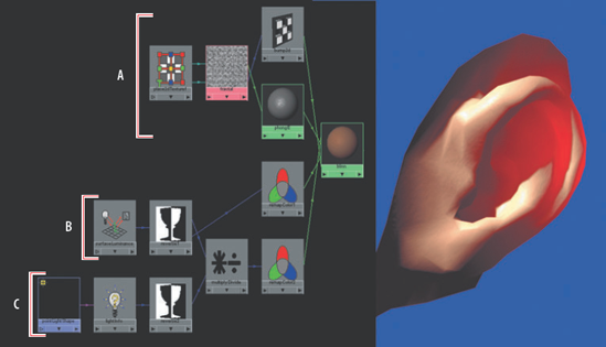
Section A provides light-colored flesh to a polygon ear. The color is supplied by a Blinn material that has a Fractal texture mapped to its Specular Color and Bump Mapping attributes. This creates the illusion of fuzz and pores. The specular information is passed to the blinn node by a phongE material node. The outColor of the fractal texture node is connected to the specularColor of the phongE node. The outColor of the phongE node is connected to the specularColor of the blinn node. By plugging together two materials that possess different attributes, you achieve a hybrid material. Although the blinn node does not have Roughness and Highlight Size attributes, it inherits their qualities from the phongE node. You can use this technique to pass Color, Ambient Color, Incandescence, and Transparency information between materials.
Section B creates a low red ambience for the ear. The ambience occurs on those polygons that receive little illumination from the scene's spot light. This is achieved by connecting the outValue of a surfaceLuminance utility node to the inputX of a reverse node name reverse1. The outputX of reverse1 is connected to the colorR of a remapColor node named remapColor1. The remapColor1's Green and Blue gradients have been flattened. The Red gradient is given a low curve. By adding a Remap Color utility, the adjustment of the ambient color becomes interactive through the use the gradients. Last, the outColor of remapColor1 node is connected to the ambientColor of the blinn node. This network causes the Ambient Color value to increase as the surface illumination intensity decreases.
Section C provides the ear with a red translucent "hot spot" where light scatters through the ear. This is purely an illusion, however, created with a Light Info utility. In this situation, a point light is positioned behind the ear. Its Intensity is set to 0 since its position is all that is needed. The worldMatrix[0] of the pointLightShape node is connected to the worldMatrix of a lightInfo node. The sampleDistance of a lightInfo node is connected to the inputX of a reverse node named reverse2. The outputX of reverse2 is connected to input1X of a multiplyDivide node. In addition, outputX of reverse1 is connected to input2X of the same multiplyDivide node. This has the effect of decreasing the sampleDistance value wherever the surfaceLuminance value is high. This ensures that the simulated translucence only occurs where the surface is unlit and is close to the point light. The outputX of the multiplyDivide node is connected to the color of a second remapColor node named remapColor2. Once again, the Green and Blue gradients are flattened. The Red gradient is given a delayed slope. This prevents the "hot spot" from becoming too strong. Last, the outColor of remapColor2 is connected to incandescence of the blinn node.
With the application of several Multiply Divide utilities, you can derive the rotation of a tire from the translation of a tire's axle. The scene in Figure A.7 is included as multiply_tire.ma on the CD in the Additional_Techniques scene folder. To view the custom network, follow these steps:
Open the Hypershade window and switch to the Utilities tab.
MMB-drag any of the multiplyDivide nodes into the work area.
With the multiplyDivide node selected, click the Input And Output Connections button. The entire network becomes visible.
In this example, the following formula is used:
rz = tz * (360 / (2 * Pi * r))
rz is the rotation of the tire on its Z axis. tz is the translation of the axle along the Z axis. r is the tire radius. Pi is the mathematical constant that represents the ratio of the circumference of a circle to its diameter. In this network, the scaleX of the transform node of the NURBS tire is connected to the input1X of multiplyDivideA. Input2X is set to 1.5 and the Operation is set to Multiply. Since the wheel has a scale of 1, 1, 1 and a diameter of 3 units, multiplying scaleX by 1.5 produces the radius (the radius being half the length of the diameter). This will allow the automation to work even if the NURBS wheel is scaled evenly in X, Y, and Z through the animation (although the axle itself cannot be scaled).
The outputX of multiplyDivideA is connected to input2X of multiplyDivideB. Input1X of multiplyDivideB is set to 6.28 and Operation is set to Multiply. This provides the (2 * Pi * r) portion of the equation; in this case, Pi is rounded to 3.14 and r is supplied by the outputX of multiplyDivideA.
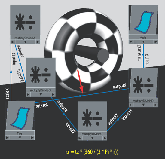
Figure A.7. A tire rotates automatically with the help of Multiply Divide utilities. The red arrow indicates the point at which a Unit Conversion utility is inserted by the program.
The outputX of multiplyDivideB is connected to input2X of multiplyDivideC. Input1X of multiplyDivideC is set to 360 and Operation is set to Divide. This provides the 360 / portion of the equation. The outputX of multiplyDivideC is connected to input2X of multiplyDivideD. The translateZ attribute of the axle shape node is also connected to input1X of multiplyDivideD. The Operation of multiplyDivideD is left on Multiply. This provides the tz * portion of the equation. Finally, the outputX of multiplyDivideD is connected to rotateX of the tire transform node. (Maya automatically inserts a Unit Conversion utility between these two nodes.) This automation will work whether the axle moves forward or backward.
With the application of a Plus Minus Average utility and several Multiply Divide utilities, the distance between the edge of an object and the furthest point of a theoretical shadow is measured. The scene in Figure A.8 is included as plus_distance.ma on the CD in the Additional_Techniques scene folder. To view the custom network, follow these steps:
Open the Hypershade window and switch to the Utilities tab.
MMB-drag the plusMinusAverage node into the work area.
With the plusMinusAverage node selected, click the Input And Output Connections button. The entire network becomes visible.
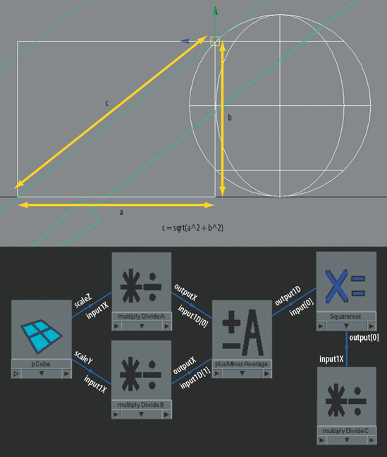
Figure A.8. The length of a triangle's edge is determined with the aid of a Plus Minus Average utility.
A directional light is scaled and placed above the center of a primitive sphere. In this position, the center line of the light glances the edge of the sphere and ends on a ground plane. To determine the distance from the point the light glances the sphere to the point the light intersects the ground (a theoretical shadow end point), you can employ the Pythagorean theorem. The theorem, which states that the square of the length of the hypotenuse of a right triangle equals the sum of the squares of the lengths of the other two sides, is often represented by this equation:
a^2 + b^2 = c^2
The theorem can also be used to determine the length of the hypotenuse:
square root of (a^2 + b^2)
One quick and dirty way to derive the length of the two sides that form the right angle is to place a primitive cube in the scene. In this case, a polygon cube is scaled and translated so that it forms a virtual right triangle with sides a, b, and c. The scaleZ attribute of the pCube transform node is connected to the input1X of a multiplyDivide node (multiplyDivideA). The scaleY attribute is connected to the input1X of a second multiplyDivide node (multiplyDivideB). Each multiplyDivide node has its Operation set to Power and 2 entered into the Input2X field. Since the transforms of pCube were never frozen, the scales represent the cube's actual world size. scaleZ of pCube thus corresponds to the length of the triangle's side a, while the pCube's scaleY corresponds to side b.
The outputX of multiplyDivideA is connected to the input1D[0] of a plusMinusAverage node. The outputX of multiplyDivideB is connected to the input1D[1] of the plusMinusAverage node. The plusMinusAverage node Operation is set to Sum. These three utilities provide the a^2 + b^2 portion of the equation. The next step, which requires a square root, necessitates an expression. The output1D of the plusMinusAverage node is connected to the input[0] of an Expression node (Squareroot). The expression follows:
multiplyDivideC.input1X=sqrt(plusMinusAverage.output1D);
Finally, as a test, the output[0] of Squareroot is connected to a third multiplyDivide node (multiplyDivideC). The length of the hypotenuse (side c) can be seen in the Input1X field of this last node. Although you can use the Distance tool to derive such a length, this example demonstrates the trigonometric capabilities of Plus Minus Average and Multiply Divide utilities. (For more information on the use of expressions in custom networks, see "A Note on Expressions" in Chapter 8.)
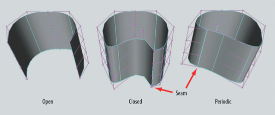
When a NURBS surface is closed or made periodic, issues can arise from the resulting distribution of the UV texture space. Before discussing the ramifications, I need to define open, closed, and periodic surfaces.
- Open
A surface in which the start and end edit points are in different positions. The scene in Figure A.9 is included as
closed_periodic.maon the CD in the Additional_Techniques scene folder.- Closed
A surface in which the start and end edit points coincide (see Figure A.9). In this situation, coinciding edit points share the same position in space and are displayed as a single edit point. Vertices also coincide at the seam. However, you can separate pairs of vertices with the Move tool. Once the vertices are repositioned, the surface is no longer closed and is considered open.
- Periodic
A surface that appears similar to a closed surface, but maintains continuity (that is, a smooth transition of the surface between the edit points). This is achieved by creating two additional spans that overlap the start and end edit points but that cannot be seen (see Figure A.9).
A quick way to determine whether a surface is closed or periodic is to check the Form U and Form V attributes, which are located in the NURBS Surface History section of the surface's shape node Attribute Editor tab. Form U and Form V display the words Open, Closed, or Periodic and will update instantly if the surface changes.
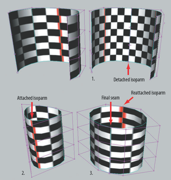
If it becomes necessary to make a NURBS surface periodic, you can choose Edit NURBS > Open/Close Surfaces. However, the UVs of the surface will be drastically affected. For example, in Figure A.10, step 1, a lofted surface has the Open/Close Surfaces tool applied with default settings. The UV texture space taken up by the original final span is thus spread across the three new spans. The center line, represented by a red line from a Ramp texture, has shifted slightly.
Note
Although the Open/Close Surfaces tool includes the word Close in its name, the result is always a periodic surface. To create a closed surface, you must select the isoparm that forms the seam of a periodic surface and choose Edit NURBS > Detach Surfaces. When you do so, additional vertices appear.
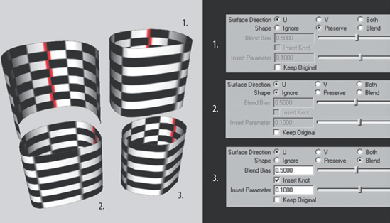
Figure A.10. Multiple applications of the Open/Close Surfaces tool. The open surface used in this demonstration is included as open_surface.ma on the CD in the Additional_Techniques scene folder.
In Figure A.10, step 2, the Open/Close Surfaces tool is applied with Shape set to Ignore and Surface Direction set to U. In this case, Open/Close Surfaces makes no attempt to maintain the surface's original shape; hence, the surface loop becomes tighter. The center line is shifted to an even greater degree. The resulting surface also has seven spans.
In Figure A.10, step 3, the Open/Close Surfaces tool is applied with Shape set to Blend and Insert Knot checked. The Blend option attempts to maintain continuity (the smooth transition across the seam). The result is similar to step 2. However, the surface has six spans. If Insert Knot is unchecked, the resulting surface maintains the original four spans but forms an even tighter loop.
To avoid the heavy shifting of UVs, it's best to close only small gaps with the Open/Close Surfaces tool. Another way to convert an open surface to a closed surface without adversely affecting the surface's UVs involves attaching and detaching surface isoparms. Using the open_surface.ma file in the Additional_Techniques scene folder of the CD, you can follow these three steps:
Select the midpoint isoparm on the surface. Use Figure A.11 as a reference. Choose Edit NURBS > Detach Surfaces >

Select the two isoparms on the two ends. Choose Edit NURBS > Attach Surfaces >
Select the two isoparms at the midpoint that were detached in step 1. Choose Edit NURBS > Attach Surfaces >
Note
Maya has a tendency to forget that a surface is closed when a file is saved and reopened. Oddly enough, you can avoid this problem by turning off Construction History when applying the Attach Surfaces tool. If Construction History is left on, Attach Surfaces hides the original surface shape nodes, which interferes with the open and closed status.
High-quality render settings cannot disguise limitations of geometry. If a NURBS surface is constructed with a limited number of spans, faceting will appear along the surface edge (this is called "nickeling"). Although it is best to anticipate this issue during the NURBS modeling phase, you can adjust the tessellation (the subdivision of faces in a predictable pattern) at the point of render. Before you attempt to do so, however, familiarize yourself with Maya's display settings.
In Maya, three NURBS display settings are accessible by using hot keys (see Figure A.12). The 1 key toggles Low Quality Display, the 2 key toggles Medium Quality Display, and the 3 key toggles High Quality Display. If the workspace view is left in Wireframe mode, the NURBS surface isoparms appear smooth, but the number of spans changes with the display setting. If the workspace view is set to Smooth Shade All, the surface becomes faceted if Low Quality Display or Medium Quality Display is selected.
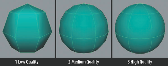
For the display setting to take effect, a NURBS surface must be selected. You can give each NURBS surface a different display setting. Low Quality Display shows the NURBS surface as if it were converted directly to a polygon surface with each NURBS edit point matching a polygon vertex. The NURBS to polygon conversion is not unusual; renderers, such as Maya Software, must convert NURBS surfaces to polygons at the point of render (although the conversion is temporary and cannot be seen in the 3D environment).
Medium Quality Display presents the surface as if each NURBS face were subdivided two times in the U and V direction. High Quality Display presents the surface as if each NURBS face were subdivided four times in the U and V direction. High Quality Display is the default display state for all new NURBS surfaces. Unfortunately, the High Quality Display setting does not correspond directly with the default NURBS tessellation used by the Maya Software renderer. For example, the Smooth Shade All view of a primitive NURBS sphere does not match a Maya software render of the same view. Thankfully, the discrepancy is fairly minor and will not impact the majority of animations. In any case, you can see the actual render tessellation in a workspace view by checking the Display Render Tessellation attribute (see Figure A.13). NURBS tessellation settings reside in the Tessellation section of the surface's shape node Attribute Editor tab.
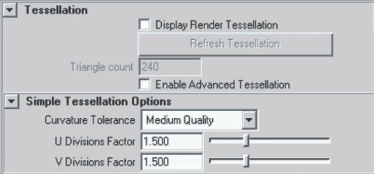
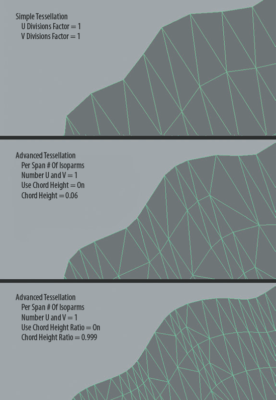
By default, a NURBS surface is given Simple Tessellation. A primitive sphere, for example, receives a U Divisions Factor and V Divisions Factor of 4.5 and a Curvature Tolerance set to Medium Quality. In this case, approximately 4.5 quadrilateral polygons are generated per NURBS face (with each quadrilateral composed of two triangles). The number of quadrilaterals is said to be approximate because the U Divisions Factor and V Divisions Factor values are affected by the Curvature Tolerance, which in turn remotely controls the Chord Height Ratio attribute.
Chord height, as a term, refers to the distance between the center of a NURBS span (which runs from edit point to edit point in a straight line) and the spline that defines a NURBS surface. In contrast, the Chord Height Ratio, as a term, represents the maximum ratio between the length of a span and the distance the center of that span is from the spline that defines a NURBS surface. If the Curvature Tolerance attribute is set to Highest Quality, the Chord Height Ratio attribute is remotely set to 0.995, which results in a smoother rendered surface. This is most obvious when U Divisions Factor and V Divisions Factor are set to a low value. If the Curvature Tolerance attribute is set to No Curvature Check, no attempt to smooth out the surface is undertaken.
In general, it's best to set the Curvature Tolerance attribute before adjusting the U Divisions Factor and V Divisions Factor. Nevertheless, the higher the value of the U Divisions Factor and V Divisions Factor attributes, the smoother the resulting render.
Simple Tessellation, while perfectly suited for most applications, fails to maintain isoparm position. That is, the resulting polygon face edges do not line up with the original NURBS isoparms. At the same time, Simple Tessellation is unable to create an adaptively light surface. Advanced Tessellation, on the other hand, does not have these limitations.
You can activate Advanced Tessellation by selecting the Enable Advanced Tessellation attribute. Additional options become available in the Primary Tessellation Attributes, Secondary Tessellation Attributes, and Common Tessellation Options sections of the surface's shape node Attribute Editor tab (see Figure A.14).
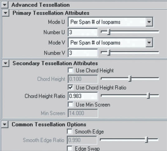
Figure A.14. The Primary, Secondary, and Common Tessellation sections of a NURBS surface's shape node Attribute Editor tab
Primary Tessellation applies tessellation to the entire surface and includes Mode U, Mode V, Number U, and Number V attributes.
- Mode U and Mode V
Determine the method by which a NURBS face is subdivided. Per Span # Of Isoparms simply subdivides every span equally and tends to yield the best results. In contrast, Per Surf # Of Isoparms ignores present isoparm position and attempts to create equally spaced triangles; the result can be chaotic. Per Surf # Of Isoparms In 3D is similar, but attempts to space the triangles in 3D space instead of parametric space; hence, the results are often cleaner. Guess Based On Screen Size scales the resulting triangles to fit an assumed optimum screen size and tends to produce heavy tessellation.
- Number U and Number V
Set the number of times a single NURBS face is subdivided in the U and V direction. If both attributes are set to 1, Mode U and Mode V are set to Per Span # Of Isoparms, and the Use Chord Height Ratio attribute is unchecked, each NURBS face receives one quadrilateral.
Secondary Tessellation is adaptive, whereby additional triangles are placed only in those areas that require high subdivision density to maintain acceptable smoothness. The attributes in this section include Chord Height, Chord Height Ratio, and Use Min Screen, all of which become accessible when Enable Advanced Tessellation is checked on.
- Chord Height
If a measured chord height is greater than the Chord Height attribute value, the span and its associated polygon triangle are subdivided (see Figure A.15). In short, the lower the attribute value, the more accurate and dense the resulting tessellation. The Chord Height attribute is measured in object space. Thus, surfaces that are constructed at a small scale might tessellate inaccurately. If this should happen, the Chord Height Ratio attribute should be used instead.
- Chord Height Ratio
Represents the maximum ratio between the length of a span and the distance the center of that span is from the spline that defines a NURBS surface. When Simple Tessellation is used, this attribute is remotely controlled by Curvature Tolerance. The higher the attribute value, the more accurate and dense the resulting tessellation (see Figure A.15).
- Use Min Screen
Bases tessellation on the size of polygon triangles in screen space. A default value of 14 will ensure that no triangle is larger than 14 × 14 pixels. If a triangle exceeds the threshold, it is subdivided into additional triangles. The Use Min Screen attribute should not be used for animated objects, since the tessellation will change over time and will tend to "pop."
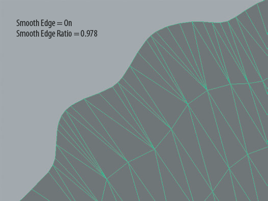
Common Tessellation is span-based and includes Smooth Edge, Smooth Edge Ratio, and Edge Swap attributes. Smooth Edge creates additional triangles along edges and boundaries (see Figure A.16). The Smooth Edge Ratio attribute controls the level of detail. Higher values create more triangles. The Edge Swap attribute, when checked, chooses the opposite set of vertices on a quadrilateral when adding the interior edge to produce two triangles; this only takes effect if the result is superior to the original triangles.
You can set tessellation per NURBS surface or universally apply the tessellation to all NURBS surfaces by switching to the Rendering menu set and choosing Render > Set NURBS Tessellation >
If Tessellation Mode is set to Manual and Manual Mode is set to Advanced, Advanced Tessellation options become available. If Tessellation Mode is left on Automatic, the tessellation is based on screen coverage, the distance from the camera to the surface, and the Curvature Tolerance, U Division Factor, and V Division Factor attributes. The Use Frame Range attribute determines which frames are evaluated for the Automatic tessellation. The result of the Set NURBS Tessellation tool is not visible in the viewport; however, the settings are applied in the Render View window or through a batch render.

A set of specialized tools are provided by mental ray to help solve rendering problems. The tools are located in the Diagnostics section of the mental ray tab in the Render Settings window (see Figure A.18).
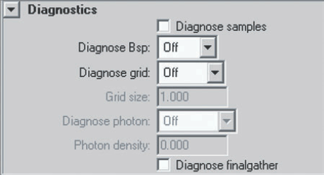
Diagnose Samples, Diagnose Bsp, and Diagnose Grid attributes tackle global rendering issues. Diagnose Finalgather and Diagnose Photon examine Final Gather and Global Illumination renders, respectively. Details of each attribute's functionality follow:
- Diagnose Samples
When checked, creates a stylized representation of subpixel sampling as instigated by the Min Sample Level, Max Sample Level, and Contrast Threshold attributes. Subpixels are indicated by white dots. High-density areas of dots signify a high degree of recursive subpixel sampling (see Figure A.19). This attribute functions with or without raytracing, Global Illumination, and Final Gather.
- Diagnose Bsp
Renders a color representation of the mental ray binary space partitioning (BSP) algorithm. A BSP algorithm is designed to accelerate raytrace renders by recursively dividing 3D space into sets of nested voxels. When the Diagnose Bsp attribute is set to Depth or Size, rendered red and/or white pixels indicate areas of the scene that are pushing the raytrace renderer to its operational limit.
- Diagnose Grid
Renders a grid on each surface in the scene. This attribute provides a quick way to measure objects without returning to a workspace view. Diagnose Grid can be set to object, world, or camera units. If Diagnose Grid is set to Camera, the grid is projected from the view of the camera. The Grid Size attribute sets the size of the grid squares. This attribute functions with or without raytracing, Global Illumination, and Final Gather.
- Diagnose Finalgather
When checked, adds to the render green and red dots that represent Final Gather points (see Figure A.20). Green dots represent initial points and red dots represent additional points created at the final stages of the render. You can use this attribute to help determine appropriate values for Falloff Start, Falloff Stop, and Max Trace Depth attributes and to assist in the even distribution of Final Gather points.
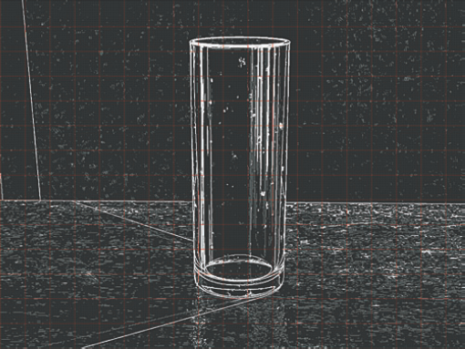
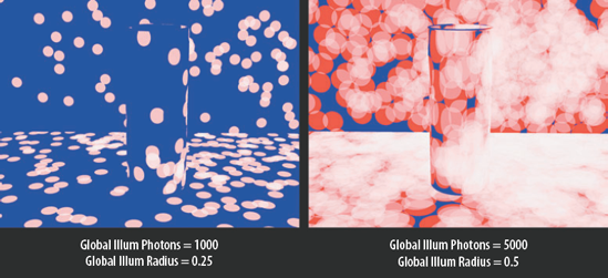
- Diagnose Photon
Shows a false-color map of photon hits (see Figure A.21). Diagnose Photon is available if Global Illumination and/or Caustics attributes are checked on in the Secondary Effects subsection of the Rendering Features section. If Diagnose Photon is set to Density, photon density is illustrated. If Diagnose Photon is set to Irradiance, red, green, and blue components of photon energy are indicated. The Photon Density attribute controls the level of detail in the test render. The higher the value, the more transparent the photon hits and the greater the false color range. You can use Diagnose Photon to help determine the proper photon Radius and Global Illum Photons attributes of a scene.