
Chapter 19
Short-term decision making
‘So there I was, fresh from the annual meeting of the Society for Judgement and Decision Making, and behaving like Buridan's Ass – the imaginary creature which starved midway between two troughs of hay because it couldn't decide which to go for.’
Source: Peter Aytan, Ditherer's Dilemma, New Scientist, 12 February 2000, p. 47.

Learning Outcomes
After completing this chapter you should be able to:
- Explain the nature of short-term business decisions.
- Understand the concept of contribution analysis.
- Investigate some of the decisions for which contribution analysis is useful.
- Draw up break-even charts and contribution graphs.
 Go online to discover the extra features for this chapter at www.wiley.com/college/jones
Chapter Summary
- In business, decision making involves choosing between alternatives and involves looking forward, using relevant information and financial evaluation.
- Businesses face a range of short-term decisions such as how to maximise limited resources.
- It is useful to distinguish between costs that vary with production or sales (variable costs) and costs that do not (fixed costs).
- Revenue less variable costs equals contribution.
- Contribution less fixed costs equals net profit.
- Contribution and contribution per unit are useful when making short-term business decisions.
- Contribution analysis can help determine which products or services are most profitable, which are making losses, whether to buy externally rather than make internally and how to maximise the use of a limited resource.
- Throughput accounting attempts to remove bottlenecks from a production system; it treats direct labour and variable overheads as fixed.
- Break-even analysis shows the point at which a product makes neither a profit nor a loss.
- Both break-even charts and contribution graphs are useful ways of portraying business information.
Introduction
Businesses, like individuals, are continually involved in decision making. A decision is simply a choice between alternatives. It is forward looking. Business decisions may be long-term strategic ones about raising long-term finance or capital expenditure. Alternatively, the decisions may be short-term, day-to-day, operational ones, such as whether to continue making a particular product. This particular chapter looks at short-term decisions. When making short-term decisions, it is important to consider only factors relevant to the decision. Depreciation, for example, will not generally change whatever the short-term decision. It is not, therefore, included in the short-term decision-making calculations.
Decision Making
Individuals make decisions all the time. These may be short-term decisions: Shall we go out or stay in? If we go out, do we go for a meal, to the cinema or to a pub? Or long-term decisions: Shall we get married? Shall we buy a house? These decisions involve choosing between various competing alternatives.
Managers also make continual decisions about the short-term and long-term future. Shall we make a new product or not? Which product shall we make: A or B? Figure 19.1 gives some examples of short-term business decisions. However, it is important to note the context. For example, discontinuing a product or department can have long-term consequences.

Whatever the nature of the decision, informed business decision making will share certain characteristics, such as being forward-looking, using relevant information and involving financial evaluation.
(a) Forward-looking
Decisions look to the future and, therefore, require forward-looking information. Past costs that have no ongoing implications for the future are irrelevant. These costs are sometimes known as sunk costs and should be excluded from decision making.
(b) Relevant Information
When choosing between alternatives, we are concerned only with information which is relevant to the particular decision. For example, after arriving in the centre of town by taxi, you are trying to choose between going to the cinema or pub. The taxi fare is a sunk cost which is not relevant to your decision. You cannot alter the past. Relevant costs and revenues are, therefore, those costs and revenues that will affect a decision. Sunk costs are non-relevant costs.
To make an informed decision only relevant information is needed. This information may be financial or non-financial. The non-financial information will normally, however, have indirect financial consequences. For example, a drop in the birth rate may have financial consequences for suppliers of baby products.
(c) Financial Evaluation
In business, effective decision making will involve financial evaluation. This means gathering the relevant facts and then working out the financial benefits and costs of the various alternatives. There are a variety of techniques available to do this, which we will be discussing in subsequent chapters.
Decisions may have opportunity costs. Opportunity costs are the potential benefit lost by rejecting the best alternative course of action. If you work in the union bar at £9 per hour and the next best alternative is the university bookshop at £7 per hour, then the opportunity cost is £7 per hour. This is because you forgo the chance of working in the bookshop at £7 per hour. However, from the above, it should not be assumed that business decision making is always wholly rational. As we all know, many factors, not all of them rational, enter into real-life decision making (see Real-World View 19.1).
 REAL-WORLD VIEW 19.1
The upshot? Although you might think that asking what you want should be the flip-side of asking what you don't want, it isn't. When you reject something you focus more on the negative features; when you select something you're focusing on the positive. So whether it's an ice cream or a prospective employee, deciding what (or who) you want by a process of rational elimination may not actually give you what you want. There is no simple panacea to ease the pain of choice other than passing the buck, of course (hence the irksome cliché: ‘No, you decide’).
As for you sadistic purveyors of all this choice, don't get too smug. When Sheena Sethilyengar, from the Massachusetts Institute of Technology, set up a tasting counter for exotic jams in a grocery, she found that too much choice can be bad for business. More customers stopped to sample from a 24-jam counter than from a 6-jam counter. But only 3 per cent bought any jam when 24 were on offer, compared with 30 per cent when there were 6 to choose from.
Source: Peter Aytan, Ditherer's Dilemma, New Scientist, 12 February 2000, vol. 165, no 2225, p. 471. © 2000 Reed Business Information Ltd, England Reproduced by Permission. http://www.newscientist.com/article/mg16522254.700-ditherers-dilemma.html.
Contribution Analysis
When making short-term decisions, a technique called contribution analysis has evolved. This technique has several distinctive features (see Figure 19.2).

It is now important to look more closely at the key elements of contribution analysis: fixed costs, variable costs and contribution. The analysis and interaction of these elements is sometimes called cost-profit-volume analysis. In this book, the term contribution analysis is used because it is considered easier to understand and more informative. The key difference between profit and contribution is that when determining profit you do not split the costs between fixed and variable costs. Contribution, however, is revenue less only variable costs. It is, therefore, necessary to analyse costs into those that are fixed and those that are variable. In practice, this may prove very difficult and is obviously subjective.
(i) Fixed Costs
Fixed costs do not change if we sell more or less products or services. They are thus irrelevant for short-term decisions. For a business, fixed costs might be business rates, depreciation, insurance or rent. On a normal household telephone bill, for example, the fixed cost is the amount of the rental. It should be stressed that fixed costs will not change over the short term, but over the long term all costs will change (see Pause for Thought 19.1).
 PAUSE FOR THOUGHT 19.1
Fixed Costs
In the long run all fixed costs are variable. Why do you think this is so?
This is because at some stage the underlying conditions will change. For example, at a certain production level it will be necessary to buy extra machines; this will necessitate extra depreciation and insurance, both normally fixed costs. Alternatively, if a factory closes then even the fixed costs will no longer be incurred.
(ii) Variable Costs
These costs do vary with the level of production or service provided. They are thus relevant for short-term decisions. If we take a business, variable costs might be direct labour, direct materials, or overheads directly linked to service or production. In practice, it may be difficult to ascertain which costs are fixed and which are variable. In addition, some costs will have elements of both a fixed and variable nature. For example, an electricity bill has a fixed standing charge and then an amount per unit of electricity used. However, to simplify matters, we shall treat costs as either fixed or variable.
(iii) Contribution
Contribution to fixed overheads, or contribution in short, is simply revenue less variable costs. If revenue is greater than variable costs, it means that for each product made or service provided the business contributes to its fixed overheads. Once a business's fixed overheads are covered, a profit will be made.
Contribution, as we shall see, is a very useful technique which enables businesses to choose the most profitable goods and services. Contribution analysis is sometimes called marginal costing. This comes from economics where a marginal cost is the extra cost or ‘incremental’ cost needed to produce one more good or service. Figure 19.3 demonstrates how contribution analysis works.
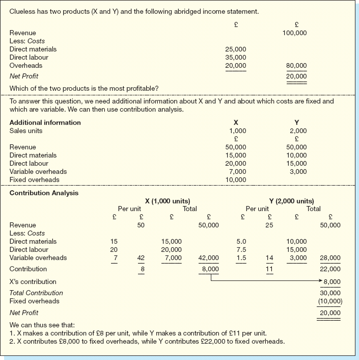
The contribution data in Figure 19.3 can be used to answer a series of ‘what if’ questions, varying the levels of sales for X and Y. Contribution analysis is thus very versatile (as Figure 19.4 shows).

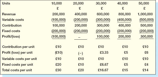
Cost Behaviour
Understanding cost behaviour is extremely important as it affects not only contribution, but profit. Let us take the example of Costbehav Ltd which manufactures widgets. It is planning production for the next year. It is considering five levels of production: 10,000, 20,000, 30,000, 40,000 or 50,000 units per year. Sales will be £2 per unit. Fixed costs are £200,000 whereas variable costs are £10 per unit. How would contribution and profit vary with production?
It can be seen by looking at Figure 19.5 that contribution per unit and variable cost per unit remain constant. However, fixed costs per unit decline from £20 to £4 while total costs fall from £30 per unit to £14 per unit. As a result profit per unit increases from a loss of £10 at 10,000 units to a profit of £6 per unit at 50,000 units.
Decisions, Decisions
Contribution analysis can be used in a range of possible situations. All these involve the basic business questions:
- Are we maximising the firm's contribution by producing the most profitable products?
- Is the product making a positive contribution to the firm? If not, cease production.
- Should we make the products in house?
- Are we making the most of limited resources?
Although the decisions are different, the basic approach is the same (see Helpnote 19.1). In all cases, we are seeking to maximise a company's contribution.
 HELPNOTE 19.1
Basic Contribution Approach to Decision Making
- Separate the costs into fixed and variable.
- Allocate revenue and costs to different products.
- Calculate contribution (revenue less variable cost) for each product:
(a) in total; (b) where appropriate, per unit or per unit of limiting factor.
It is important to realise that contribution analysis provides a rational approach to decision making. However, it should not be seen as providing a definitive answer. In the end, making the right decision will also involve an element of judgement. This is the sentiment expressed in Soundbite 19.1.
 SOUNDBITE 19.1
‘Making the right decision is crucial in the world of business. It comes as no surprise that companies spend a lot of their training budgets on developing their staff's decision making techniques. If you make a well considered decision you will lead your team to success. On the other hand, a poor decision can end in failure.’
British Council: www.british-council.org/learnenglish
Source: As reprinted in Global Accountant Magazine, July/August 2011, p. 32. British Council.
An interesting example relates to Lego, the children's retail company. In 2005, Lego cut the number of colours by half and reduced the number of stock-keeping-units to £6,500. As Real-World View 19.2 shows, this produced tremendous results for Lego.
Reducing Product Ranges
Results for customer: While customers saw the number of product options reduced and were asked to change their ordering habits, they obtained a substantial improvement in customer service. On-time delivery rose from 62 per cent in 2005 to 92 per cent in 2008.
Customers rated Lego as a ‘best in class’ supplier and Lego won a European supply chain excellence award. Those customers were now asking their other suppliers to use Lego as the benchmark for excellence.
The result for Lego: Sales increased from 2005 to 2008 by 35 per cent and profitability in 2008 was an all-time record. The fixed cost base had been reduced from 75 per cent to 33 per cent.
Source: The case study: Lego, Financial Times, 25 November 2010, p. 16. Copyright IMD. (Carlos Cordon, Ralf Seifert and Edwin Wellian)
(i) Determining the Most Profitable Products
If a company makes a range of products or services, we can use contribution analysis to see which are the most profitable (see Figure 19.6).
(ii) Should We Cease Production of Any Products?
The key here is to see whether or not any products or services are making a negative contribution. If they are, this will decrease our overall contribution.

Negative Contribution
Why should we discontinue any product or service with a negative contribution?
Products and services with negative contribution are bad news. This means that every extra product or service makes no contribution to our fixed costs. In actual fact, the more products or services we provide the greater our loss. This is because our variable costs per unit are greater than the selling price per unit.
Let us take the example in Figure 19.7.
A key aspect of discontinuing a product is the identification of complementary goods (e.g., eggs and bacon, fish and chips) where if one discontinues one product then you will lose sales of the other.

(iii) The Make or Buy Decision
Here we need to compare the cost of providing goods or services internally with the cost of buying in the goods or services. We compare the variable costs of making them internally with the external costs. Businesses often outsource (i.e., buy in) their non-essential activities. In Real-World View 19.3, the role of outsourcing is discussed after the British General Election of May 2010.
British Airways and Outsourcing
Outsourcing is a popular way in which companies can attempt to cut their costs. Although the sector in the UK suffered following the May 2010 election, J. Ficenec (2011) shows outsourcing has subsequently increased in the UK with, for example, back-office outsourcing expert Capita announcing a £1.1bn of major contracts in the first six months of 2011.
‘These new opportunities and the increase in business activity come as the government desperately tries to get its finances under control.’
Source: J. Ficenec (2011) Outsourcing Austerity, Investors Chronicle (14–20 October, p. 54). Financial Times.
This sort of decision is also often faced by local governments in tendering or contracting out services such as cleaning (see Figure 19.8).

Other Factors in Make or Buy Decisions
What other factors, apart from the costs, should you take into account in make and buy decisions?
In practice, make or buy decisions can involve many other factors. For example:
- Have the internal employees other work?
- Is the external price sustainable over time?
- Do we want to be dependent on an external provider?
- Will we be able to take action against the external provider if there is a deficient service?
- What consequences will awarding the contract externally have for morale, staff turnover?
(iv) Maximising a Limiting Factor
Businesses often face a situation where one of the key resource inputs is a limiting factor on production. For example, the quantity of direct materials may be limited or labour hours may be restricted. The basic idea, in this case, is to maximise the contribution of the limiting factor. Figure 19.9 demonstrates this concept for a hotel which has three restaurants, but a limited amount of direct labour hours.


Throughput Accounting
Throughput accounting is a relatively new approach to production management and uses a variant of contribution per limiting factor. This approach looks at a production system from the perspective of capacity constraint or bottlenecks. It essentially asks: what are a system's main bottlenecks? For instance, is it shortage of machine hours in a certain department? Every effort is then made to eliminate the bottlenecks. Goldratt and Cox in The Goal (1992) look at throughput contribution (defined as revenue less direct materials) as a key measure. Interestingly, therefore, all other costs are treated as fixed. Thus, direct labour and variable overheads are seen as fixed overheads in this system. Figure 19.10 provides an example of a throughput operating statement. The throughput contribution is £40,000 (i.e., revenue of £105,000 less direct materials at £65,000).

Throughput analysis just like contribution per limiting factor could be used to allocate production if there was a production bottleneck. Let's just assume that three products (A, B and C) go through many processes, but process B's hours are limited. In this case, one would calculate out the contribution per process B hour, using the additional data in Figure 19.11.
Figure 19.11 shows that A has the greatest contribution, but more important the greatest contribution per process hour. It pays, therefore, to focus on product As then product B and finally product C.

Break-Even Analysis
The contribution concept is particularly useful when determining the break-even point of a firm. The break-even point is simply that point at which a firm makes neither a profit nor a loss. A firm's break-even point can be expressed as follows:
![]()
In other words, the break-even point is the point where contribution equals fixed costs.
We can find the break-even point in units by dividing fixed costs by contribution per unit. Figures 19.12 and 19.13 show how the break-even point works.


Assumptions of Break-Even Analysis
The beauty of break-even analysis is that it is comparatively straightforward. However, breakeven analysis is underpinned by several key assumptions. Perhaps the main one is linearity. Linearity assumes that the behaviour of the revenue and costs will remain constant despite increases in the level of revenue. Revenue and variable costs are assumed always to be strictly variable and fixed costs are assumed to be strictly fixed. For instance, in Figure 19.11 it is assumed that revenue will remain at £20 per meal, variable costs will remain at £8 per meal and fixed costs will remain at £120,000, whether we sell 1,000 meals, 10,000 meals or 100,000 meals. In practice, it is more likely that these costs will be fixed or variable within a particular range of activity (often called the relevant range). The break-even point also implies a precision which is perhaps unwarranted. A better description might be the break-even area. In practice, break-even analysis suffers from the same problems as contribution analysis more generally. In particular, it is difficult for accounting to estimate variable or fixed costs.
Other Uses of Break-Even Analysis
Break-even analysis can also form the basis of more sophisticated analyses such as (i) calculating the margin of safety, (ii) the basis for ‘what-if’ analysis, or (iii) the basis for graphical analysis.
(i) Margin of Safety – Purposes and Limitations
Bunter may wish to calculate how much he has sold over and above the break-even point. It can be seen as a company's comfort zone, the amount of revenue which the company could lose before it starts making a loss. This is called the margin of safety. Bunter's margin of safety is calculated using a general formula:
![]()
The break-even point can be calculated in either (a) units (i.e., in this case, meals) or (b) money. Therefore,

(ii) What-if Analysis
The break-even point can also be used as a basis for ‘what-if’ analysis. For instance, we know that each unit sold in excess of the break-even point adds one unit's contribution to profit. Similarly, each unit less than the break-even point creates a loss of one unit's contribution. So, we can easily answer questions such as ‘what is the profit or loss if Bunter sells (a) 8,000 meals or (b) 13,000 meals?’
| (a) | 8,000 meals. This is 2,000 meals less than the break-even point of 10,000 meals. The loss is, therefore, 2,000 meals × contribution per meal. Thus, 2,000 meals × £12 contribution per meal (revenue £20 − £8 variable cost) = £24,000 loss. |
| (b) | 13,000 meals. This is 3,000 meals more than the break-even point of 10,000 meals. The profit is thus 3,000 meals × £12 contribution per meal (revenue £20 − £8 variable cost) = £36,000 profit. |
The break-even point is a very flexible concept and provides potentially rewarding insights into business.
(iii) Graphical Break-Even Point
Another benefit of break-even analysis is that it can be shown on a graph (see Figure 19.14).

Figure 19.15 is the graph for William Bunter. Sales are set at four levels: 0 meals; 5,000 meals; 10,000 meals; and 15,000 meals. Break-even point is 10,000 meals.

(iv) Contribution to Revenue
Another useful technique is to evaluate different products using their contribution to revenue. Thus, if we had three different products we could rank them by their contribution to revenue as in Figure 19.16. This is often called contribution to sales, but for consistency and ease of understanding, contribution to revenue is used.
In this case our most profitable product is thus C with a contribution to revenue of 66.67%.

Contribution Graph
Contribution to revenue can also be graphed. This overcomes a limitation of the break-even chart in that it can be used for only one product. A contribution graph (see Figure 19.17) is sometimes called a profit/volume chart. However, in this book we use the term contribution graph as it is easier to understand. A contribution graph looks a bit like a set of rugby posts! It is based on the idea that each unit sold generates one unit's contribution. Initially, this contribution covers fixed costs and then generates a profit. The horizontal line represents level of revenue (either in units or £s). Above the horizontal line is profit, while below the line is loss. The diagonal line represents contribution. In effect, it is the cumulative profit or loss plotted against cumulative revenue. So when there is no revenue there is a loss (point A). This loss is, in effect, the total fixed costs. The company then breaks even at point B. At this point contribution equals fixed costs. Above point B each unit sold adds one unit of contribution to the company's profit. Finally, point C represents maximum cumulative revenue and maximum contribution.


The relationship between contribution and revenue is defined as ![]() .
.
Sometimes this is known as the profit/volume ratio. This ratio provides an easy way of comparing the contributions of different products. We take, as an example, a department store which has three departments: toys, clothes and CDs (see Figure 19.18).
In many industries, there are substantial fixed costs. In the retail industry, for example, as Real-World View 19.4 shows, the concept of break-even becomes very important.
Fixed Costs and Supermarkets
Richard Tomkins (Marketing Value for Money) commented on the UK supermarket chains of Asda, Safeway, Sainsbury and Tesco. ‘All of these supermarkets have substantial fixed costs. They depend on volume of sales. So that if one supermarket cuts their costs, the others are forced to follow. If they don't they are worried that their volumes will fall to below break-even point.’
Source: Richard Tomkins, Marketing Value for Money, Financial Times, 14 May 1999.
Conclusion
Businesses constantly face short-term decisions such as how to maximise a limited resource. When making these decisions it is useful to distinguish between fixed and variable costs. Fixed costs do not, in the short run, change with either production or revenue (for example, insurance or depreciation). Variable costs, by contrast, do change when the production volume or revenue volume changes (examples are direct materials and direct labour). Revenue (sales) less variable costs gives contribution. Contribution is a useful accounting concept. By calculating contribution we can, for example, determine which products are the most profitable. Break-even analysis is another useful concept that builds on contribution analysis. The break-even point is the point at which a business makes neither a profit nor a loss. It is determined by dividing fixed costs by the contribution per unit. The break-even chart shows the break-even point graphically. The contribution graph is a useful way of graphing the profit or loss of one or more products.
 Discussion Questions
Questions with numbers in blue have answers at the back of the book.
| Q1 | Distinguish between fixed and variable costs. Why are fixed costs irrelevant when making a choice between certain alternatives such as whether to produce more of product A or of product B? |
| Q2 | What is contribution per unit and why is it so useful in short-term decision making? |
| Q3 | What are the strengths and weaknesses of break-even analysis? |
| Q4 | State whether the following statements are true or false? If false, explain why.
(a) Fixed costs are those that do not vary with long-term changes in the level of revenue or production. (b) Contribution is revenue less variable costs. (c) Break-even point is (d) Contribution/revenue (sales) ratio is (e) Non-financial items are not important in decision making. |
Numerical Questions
Questions with numbers in blue have answers at the back of the book.


Go online to discover the extra features for this chapter at www.wiley.com/college/jones