CHAPTER 12
Risk in the Real World
THE CHALLENGE
G. H. Hardy, the legendary mathematician, once claimed that his greatest disappointment in life was learning that someone had discovered an application for one of his theorems. Although Hardy's disinterest in practical matters was a bit extreme, it sometimes seems that scholars view the real world as an uninteresting special case of their models. This disinterest in real‐world complexity, unfortunately, often brings unpleasant consequences. In this chapter, we address two simplifications about risk that often lead investors to underestimate their portfolios' exposure to loss. First, investors typically measure risk as the probability of a given loss, or the amount that can be lost with a given probability, at the end of their investment horizon, ignoring what might occur along the way. Second, they base these risk estimates on return histories that fail to distinguish between calm environments, when losses are rare, and turbulent environments, when losses occur more commonly. In this chapter, we show how to estimate exposure to loss in a way that accounts for within‐horizon losses as well as the regime‐dependent nature of large drawdowns.
END‐OF‐HORIZON EXPOSURE TO LOSS
Probability of Loss
We measure the likelihood that a portfolio will experience a certain percentage loss at the end of a given horizon by computing the standardized difference between the percentage loss and the portfolio's expected return, and then converting this quantity to a probability by assuming returns are normally distributed. Unfortunately, asset class returns are not normally distributed. Returns tend to be lognormally distributed, because compounding causes positive cumulative returns to drift further above the mean than the distance negative cumulative returns drift below the mean.1 (See Chapter 18 for more detail about lognormality.) This means that logarithmic returns, also called continuous returns, are more likely to be described by a normal distribution. Therefore, in order to use the normal distribution to estimate probability of loss we must express return and standard deviation in continuous units, as shown in Equation (12.1). We provide the full mathematical procedure for converting returns from discrete to continuous units in Chapter 18.

In Equation (12.1), ![]() equals the probability of loss at the end of the horizon,
equals the probability of loss at the end of the horizon, ![]() is the cumulative normal distribution function,
is the cumulative normal distribution function, ![]() is the natural logarithm,
is the natural logarithm, ![]() equals the cumulative percentage loss in discrete units,
equals the cumulative percentage loss in discrete units, ![]() equals the annualized expected return in continuous units,
equals the annualized expected return in continuous units, ![]() equals the number of years in the investment horizon, and
equals the number of years in the investment horizon, and ![]() equals the annualized standard deviation of continuous returns.
equals the annualized standard deviation of continuous returns.
Value at Risk
Value at risk gives us another way to measure a portfolio's exposure to loss. It is equal to a portfolio's initial wealth multiplied by a quantity equal to expected return over a stated horizon minus the portfolio's standard deviation multiplied by the standard normal variable2 associated with a chosen probability. Again, we express return and standard deviation in continuous units. But we convert the continuous percentile return (![]() ) to a discrete return before multiplying it by initial wealth, as shown in Equation (12.2). As Equations (12.1) and (12.2) reveal, probability of loss and value at risk are flip sides of the same coin.
) to a discrete return before multiplying it by initial wealth, as shown in Equation (12.2). As Equations (12.1) and (12.2) reveal, probability of loss and value at risk are flip sides of the same coin.
Here, ![]() equals value at risk,
equals value at risk, ![]() equals the annualized expected return in continuous units,
equals the annualized expected return in continuous units, ![]() equals the number of years in the investor's horizon,
equals the number of years in the investor's horizon, ![]() is the inverse cumulative normal distribution function evaluated at a given probability level,
is the inverse cumulative normal distribution function evaluated at a given probability level, ![]() equals the annualized standard deviation of continuous returns, and
equals the annualized standard deviation of continuous returns, and ![]() equals initial wealth.
equals initial wealth.
These formulas assume that we observe our portfolio only at the end of the investment horizon and disregard its values throughout the investment horizon. We argue that investors should and do perceive risk differently. They care about exposure to loss throughout their investment horizon and not just at its conclusion.
WITHIN‐HORIZON EXPOSURE TO LOSS
Within‐Horizon Probability of Loss
To account for losses that might occur prior to the conclusion of the investment horizon, we use a statistic called first passage time probability, which gives the probability that a portfolio will depreciate to a particular value over some horizon if it is monitored continuously.3 It is equal to:
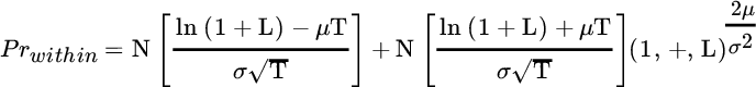
Here ![]() equals the probability of a within‐horizon loss, and the other terms are defined as they were for end‐of‐horizon probability of loss.
equals the probability of a within‐horizon loss, and the other terms are defined as they were for end‐of‐horizon probability of loss.
The first part of this equation, up to the second plus sign, gives the end‐of‐horizon probability of loss, as shown in Equation (12.1). It is augmented by another probability multiplied by a constant, and there are no circumstances in which this constant equals zero or is negative. Therefore, the probability of loss throughout an investment horizon must always exceed the probability of loss at the end of the horizon. Moreover, within‐horizon probability of loss rises as the investment horizon expands, in contrast to end‐of‐horizon probability of loss, which diminishes with time, as we discussed in Chapter 4.
Within‐Horizon Value at Risk
We use the same first passage time equation to estimate within‐horizon value at risk. Whereas value at risk measured conventionally gives the worst outcome at a chosen probability at the end of an investment horizon, within‐horizon value at risk gives the worst outcome at a chosen probability from inception to any time throughout an investment horizon. It is not possible to solve for within‐horizon value at risk analytically. We must resort to a numerical method. We set Equation (12.3) equal to the chosen confidence level and solve iteratively for ![]() . Within‐horizon value at risk equals
. Within‐horizon value at risk equals ![]() multiplied by initial wealth.
multiplied by initial wealth.
These two measures of within‐horizon exposure to loss bring us closer to the real world because they recognize that investors care about drawdowns that might occur throughout the investment horizon. But they ignore another real‐world complexity, to which we now turn.
REGIMES
Thus far we have assumed implicitly that returns come from a single distribution. It is more likely that there are distinct risk regimes, each of which may be normally distributed but with a unique risk profile. For example, we might assume that returns fit into two regimes, a calm regime characterized by below‐average volatility and stable correlations, and a turbulent regime characterized by above‐average volatility and unstable correlations. The returns within a turbulent regime are likely to be event driven, whereas the returns within a quiet regime perhaps reflect the simple fact that prices are noisy.
We detect a turbulent regime by observing whether or not returns across a set of asset classes behave in an uncharacteristic fashion, given their historical pattern of behavior. One or more asset class returns, for example, may be unusually high or low, or two asset classes that are highly positively correlated may move in the opposite direction.
There is persuasive evidence showing that returns to risk are substantially lower when markets are turbulent than when they are calm. This is to be expected, because when markets are turbulent investors become fearful and retreat to safe asset classes, thus driving down the prices of risky asset classes. This phenomenon is documented in Table 12.1.
TABLE 12.1 Conditional Annualized Returns to Risky Assets January 1976–December 2015
| 10% Most Turbulent Months | Other 90% | |
| U.S. Equities | −5.5% | 13.7% |
| Foreign Developed Market Equities | –10.0% | 13.1% |
| Emerging Market Equities | −43.0% | 20.4% |
| Commodities | –12.5% | 8.2% |
This description of turbulence is captured by a statistic known as the Mahalanobis distance. It is used to determine the contrast in different sets of data. In the case of returns, it captures differences in magnitude and differences in interactions, which can be thought of, respectively, as volatility and correlation surprise.
In Equation (12.4), ![]() equals a set of returns for a given period,
equals a set of returns for a given period, ![]() equals the historical average of those returns, and
equals the historical average of those returns, and ![]() is the historical covariance matrix of those returns.
is the historical covariance matrix of those returns.
The term ![]() captures extreme price moves. By multiplying this term by the inverse of the covariance matrix, we capture the interaction of the returns, and we render the measure scale independent as well. We multiply by
captures extreme price moves. By multiplying this term by the inverse of the covariance matrix, we capture the interaction of the returns, and we render the measure scale independent as well. We multiply by ![]() so that the average turbulence score across the data set equals 1. We illustrate this concept with a scatter plot of U.S. and foreign equities shown in Figure 12.1.
so that the average turbulence score across the data set equals 1. We illustrate this concept with a scatter plot of U.S. and foreign equities shown in Figure 12.1.

FIGURE 12.1 Scatter Plot of U.S. and Foreign Equities
Each dot represents the returns of U.S. and foreign equities for a particular period, such as a day or a month. The center of the ellipse represents the average of the joint returns of U.S. and foreign equities. The observations within the ellipse represent return combinations associated with calm periods, because the observations are not particularly unusual. The observations outside the ellipse are statistically unusual and therefore likely to characterize turbulent periods. Notice that some returns just outside the narrow part of the ellipse are closer to the ellipse's center than some returns within the ellipse at either end. This illustrates the notion that some periods qualify as unusual not because one or more of the returns was unusually high or low but, instead, because the returns moved in the opposite direction that period despite the fact that the asset classes are positively correlated, as evidenced by the positive slope of the scatter plot.
This measure of turbulence is scale independent in the following sense. Observations that lie on a particular ellipse all have the same Mahalanobis distance from the center of the scatter plot, even though they have different Euclidean distances.
We suggest that investors measure probability of loss and value at risk not based on the entire sample of returns but, rather, on the returns that prevailed during the turbulent subsamples, when losses occur more commonly. This distinction is especially important if investors care about losses that might occur throughout their investment horizon, and not only at its conclusion.
Full‐Sample versus Regime‐Dependent Exposure to Loss
Recall the moderate portfolio we derived in Chapter 2. It had an expected return of 7.5 percent and a standard deviation of 10.8 percent. Given a confidence level of 1 percent and based on a sample of returns beginning in January 1976 and ending in December 2006, without any knowledge of the pending global financial crisis, and using the conventional approach to estimating value at risk, we would have concluded that this portfolio had a 1 percent chance of losing as much as 14.2 percent of its initial value at the end of a five‐year investment horizon.
If we had segregated the 20 percent most turbulent months from the same 30‐year history leading up to the global financial crisis, and used this information to estimate exposure to loss throughout the investment horizon and not just at its conclusion, we would have instead concluded that this same portfolio had a 1 percent chance of losing as much as 45 percent of its starting value, as shown in the bottom right quadrant of Table 12.2. In fact, this portfolio lost 35.9 percent of its value during the global financial crisis.
TABLE 12.2 Value at Risk (1%)
| Full Sample | Turbulent Regime | |
| End of horizon | –14.2% | –38.6% |
| Within horizon | –29.3% | –45.0% |
Table 12.3 shows that, based on the conventional approach for estimating probability of loss, we would have concluded that such a loss had no reasonable chance of occurrence. But again, if we recognized that losses typically occur during turbulent periods, and we considered outcomes that might occur along the way, we would have estimated that this portfolio had nearly a 5 percent chance of experiencing such a large drawdown, as we show in Table 12.3.
TABLE 12.3 Probability of 35.9% or Greater Loss
| Full Sample | Turbulent Regime | |
| End of horizon | 0.0% | 1.4% |
| Within horizon | 0.0% | 4.7% |
THE BOTTOM LINE
Investors dramatically underestimate their portfolios' exposure to loss, because they focus on the distribution of returns at the end of the investment horizon and disregard losses that might occur along the way.
Moreover, investors base their estimates of exposure to loss on full‐sample standard deviations, which obscure episodes of higher risk that prevail during turbulent periods. It is during these periods that losses are likely to occur. Complexity is inconvenient but not always unimportant.
REFERENCES
- S. Karlin and H. Taylor. 1975. A First Course in Stochastic Processes, 2nd edition (San Diego: Academic Press).
- M. Kritzman and Y. Li. 2010. “Skulls, Financial Turbulence and Risk Management,” Financial Analysts Journal, Vol. 66, No. 5 (September/October).