CHAPTER 10
Currency Risk
THE CHALLENGE
Most investors recognize that it is possible to reduce the risk of a global portfolio by hedging some portion of its foreign currency exposure, but they face the challenge of determining which currencies to hedge, how much to hedge, and what instruments to use. Some investors choose not to hedge at all. In this chapter, we evaluate the prevailing arguments for and against currency hedging. We show how to derive a range of linear and nonlinear hedging strategies, and we evaluate their impact on expected portfolio performance. Finally, we review the economic rationale that explains why the risk‐minimizing currency‐hedging policy varies across currencies and home countries.
WHY HEDGE?
Investors who chose not to hedge foreign currency exposure typically rationalize their decision by making one or both of the following assertions:
 In the long run, currencies revert to the mean, and their returns wash out. We have a long investment horizon. So why bother?
- Currencies introduce diversification to the portfolio. We want to retain this diversification rather than hedge it away.
There is ample evidence to contradict the first assertion. For example, the British pound declined from USD 4.96 in 1850 to approximately USD 1.30 in September 2016. As we write this chapter, in the wake of the historic “Brexit” vote to leave the European Union, we do not know any investors who are forecasting that the pound will revert to its mid‐nineteenth‐century levels. Moreover, there is compelling evidence to suggest that currency hedging reduces risk even over much shorter horizons. Schmittmann (2010) evaluates the benefits of hedging diversified equity and fixed‐income portfolios over the period from 1975 through 2009. For investors based in the United States, Germany, Japan, and the United Kingdom, he finds that hedging currency exposure reduces portfolio risk significantly for periods of up to five years.
Even if exchange rates do revert to the mean over the long run, it does not necessarily follow that hedging is inappropriate. To survive in the long run, investors must endure whatever losses they encounter along the way. Few investment boards meet only once, at the end of the investment horizon. Most are interested keenly in interim performance. In many cases, as we soon demonstrate, investors reduce significantly their exposure to within‐horizon losses by hedging currency exposure. Indeed, if we accept that we cannot predict the direction of currency moves, there seems to be little reason not to hedge away all of the risk that currencies introduce.
What about the diversification argument? Investors often overestimate the diversification benefits of currencies, because they focus mistakenly on the correlation between the returns of a particular foreign currency, denominated in the investor's home currency, and the returns of a foreign asset, denominated in its local currency. This correlation is often quite low. However, it does not measure properly the diversification that the foreign currency introduces to the portfolio. The relevant correlation is that between the foreign currency and the foreign asset, both denominated in the investor's home currency. This correlation is always higher, because a component of the foreign asset's return comes directly from the need to translate investment value back to one's home currency at an uncertain future exchange rate. Consider an example from Chen, Kritzman, and Turkington (2015). The correlation between U.K. equities (as measured by the returns of the MSCI U.K. Index denominated in British pounds) and the dollar‐pound exchange rate was –9 percent over the period from March 1993 through March 2013. However, when both the currency and the equity index were denominated in U.S. dollars, the correlation was +48 percent.
WHY NOT HEDGE EVERYTHING?
These counterarguments may tempt some investors to hedge all of their currency exposure, particularly if they believe that currency returns will be zero in the long run. Indeed, from a return perspective, currency hedging is a zero‐sum game: A forward contract that generates a positive return for one investor generates a negative return for another.1 But hedging 100 percent of a portfolio's currency exposure is rarely the risk‐minimizing solution. Consider a straightforward scenario with one foreign asset and one currency forward contract. The variance of the hedged portfolio is given by the familiar two‐asset variance equation:
Here, ![]() is the variance of the hedged portfolio,
is the variance of the hedged portfolio, ![]() is the asset weight,
is the asset weight, ![]() is the forward contract weight,
is the forward contract weight, ![]() is the correlation between the asset and the forward contract, and
is the correlation between the asset and the forward contract, and ![]() and
and ![]() are the variances of the asset and the forward contract, respectively. If we assume that the asset weight is 100 percent, then Equation (10.1) collapses to:
are the variances of the asset and the forward contract, respectively. If we assume that the asset weight is 100 percent, then Equation (10.1) collapses to:
To identify the forward contract weight that minimizes the variance of the portfolio, we take the derivative of Equation (10.2) with respect to ![]() . This derivative is shown in Equation (10.3).
. This derivative is shown in Equation (10.3).

To calculate the minimum‐variance hedge ratio, we set this derivative equal to zero and solve for ![]() . This gives us Equation (10.4), which equals the regression beta of the asset with respect to the forward contract, as a negative value.
. This gives us Equation (10.4), which equals the regression beta of the asset with respect to the forward contract, as a negative value.
This relationship is intuitive:
- A higher correlation between the asset and the currency indicates that the currency introduces more risk and less diversification, all else being equal, and results in a higher minimum‐variance hedge ratio.
- A higher standard deviation of the currency relative to the asset indicates that we require less notional exposure to the currency to hedge the same amount of risk.
Therefore, higher currency volatility (relative to asset volatility) results in a lower minimum‐variance hedge ratio, all else being equal.
To illustrate this concept, consider the following example. Suppose that a fixed‐income portfolio with a 5 percent standard deviation is exposed to a currency with a 6 percent standard deviation and that the correlation between the portfolio and the currency is 0.60. Equation (10.4) shows that the minimum‐variance hedge ratio equals ![]() , or 50 percent.2 Figure 10.1 shows the standard deviation of the portfolio as a function of the percentage of the portfolio that is hedged. It is apparent from Figure 10.1 that the minimum‐variance hedge ratio is 50 percent.
, or 50 percent.2 Figure 10.1 shows the standard deviation of the portfolio as a function of the percentage of the portfolio that is hedged. It is apparent from Figure 10.1 that the minimum‐variance hedge ratio is 50 percent.

FIGURE 10.1 Minimum‐Variance Hedge Ratio
It is also apparent from Figure 10.1 that a hedge ratio of 100 percent does not minimize portfolio risk, given our assumptions about standard deviation and correlation. In fact, in this example, the fully hedged portfolio has the same standard deviation as the unhedged portfolio! When computing the minimum‐variance hedge ratio, it is common practice to constrain the solution to lie between 0 and 100 percent of the exposure to the currency. A hedge ratio that is lower than 0 percent increases currency exposure. A hedge ratio above 100 percent reduces currency exposure beyond the portfolio's explicit currency exposure. We examine the notion of overhedging later in this chapter.
There are two other approaches to hedging that deserve consideration: the minimum‐regret hedge ratio and the universal hedge ratio. Some investors advocate hedging 50 percent of currency exposure, regardless of the correlations and standard deviations. Proponents of this approach argue that it minimizes the potential for an investor to experience regret should either the 0 or the 100 percent hedge ratio produce the highest return ex post. We take issue with this approach for three reasons. First, it implies that investors suffer a reduction in utility when the hedging strategy underperforms but do not enjoy an increase in utility when it outperforms. Sophisticated investors maximize their expected utility given the full distribution of potential outcomes, including gains as well as losses. Second, the most prominent empirical study in support of the minimum‐regret approach is based on a flawed assumption. Gardner and Wuilloud (1995) conducted backtests to compare mean‐variance optimal hedge ratios to a constant 50 percent hedge ratio. However, they constructed the optimal hedge ratios using historical currency returns as expected returns. (Recall our critique of this assumption in Chapter 7.) Because currency returns vary widely over short horizons, this approach results in extreme hedge positions. A more reasonable approach, which is common in practice, is to assume 0 percent expected returns for currencies and identify the hedge ratios that minimize portfolio risk. Finally, should investors wish to control the risk that their hedging policy underperforms an alternative hedging policy, they can employ multirisk optimization to do so explicitly. (See Chapter 9 for details.) Kinlaw and Kritzman (2009) show how mean‐variance‐tracking error optimization minimizes simultaneously portfolio risk and the likelihood that the hedging policy will underperform the unhedged portfolio.3
The universal hedge ratio was proposed by Black (1989). He showed that, given a particular set of assumptions, all investors should hedge the same proportion of their currency exposure. In particular, he assumed that all investors have the same risk tolerance, wealth, and portfolio composition. However, as noted by Adler and Prasad (1992), these assumptions do not hold in the real world; hence, the universal hedge ratio is likely to be suboptimal for most investors.
LINEAR HEDGING STRATEGIES
The minimum‐variance hedge ratio is an example of a linear hedging strategy; the return of the hedged portfolio is a linear function of the hedged currencies' returns. Linear hedging neutralizes not only the potential losses from currencies but also the gains. In the next section, we examine nonlinear hedging strategies, which preserve the upside potential currencies bring to the portfolio while also protecting against losses. Table 10.1 summarizes six linear hedging strategies that we evaluate in this chapter and the upper bound constraints associated with each. The lower bound for all of these hedging strategies is 0 percent because we do not want to take positions that increase currency exposure.
TABLE 10.1 Linear Hedging Strategies and Their Constraints
| Linear Hedging Strategies | Asset Weight Constraints | Currency‐Hedging Constraints | ||
| Unhedged | Fixed | Each hedge position | = | 0 |
| Full Hedging | Fixed | Each hedge position | = | Portfolio exposure to each currency |
| Currency‐Specific Hedging | Fixed | Each hedge position | ≤ | Portfolio exposure to each currency |
| Allow Cross‐Hedging | Fixed | Total hedge positions | ≤ | Portfolio's total currency exposure |
| Allow Overhedging | Fixed | Total hedge positions | ≤ | 100% |
| Allow Asset Reallocation | Variable | Total hedge positions | ≤ | 100% |
Currency‐specific hedging is an extension of minimum‐variance hedging, but it is more efficient because it is less constrained. It identifies an individual hedge ratio for each currency rather than a uniform hedge ratio across all currencies. The investor therefore retains some exposure to currencies that offer relatively more diversification than volatility, and hedges exposure to those that have the opposite properties. To identify the currency‐specific hedge ratios that minimize variance, we employ the same conceptual framework as we do to derive the minimum‐variance hedge ratio. However, the problem is more complex because we must solve for a vector of hedge ratios rather than a single hedge ratio. There are many more parameters to estimate: the standard deviation of each asset class, the standard deviation of each currency, the correlations between the asset classes and the currencies, and the correlations between the currencies. We solve this problem with mean‐variance analysis. Specifically, we maximize expected utility as a function of a vector of weights, as shown in Equation (10.5):
Here, ![]() is a column vector of
is a column vector of ![]() asset and currency weights,
asset and currency weights, ![]() is a row vector of expected returns, and
is a row vector of expected returns, and ![]() is the covariance matrix. The parameter
is the covariance matrix. The parameter ![]() reflects the investor's risk aversion. Because we assume that asset class weights are constrained at fixed values and expected currency returns are zero,
reflects the investor's risk aversion. Because we assume that asset class weights are constrained at fixed values and expected currency returns are zero, ![]() falls out of the equation along with the term
falls out of the equation along with the term ![]() .4
.4
Cross‐hedging and overhedging are extensions of currency‐specific hedging. To allow cross‐hedging, we constrain the total amount of hedging such that it is less than or equal to the total amount of foreign currency exposure. This strategy is less constrained than currency‐specific hedging because it may cross‐hedge one currency with another. One advantage of this approach is that it can hedge currencies that are more expensive to trade using correlated, proxy currencies that are less expensive to trade.
In the case of overhedging, we allow the total amount of hedging to exceed the amount of foreign currency exposure in the portfolio. This strategy, which hedges implicit as well as explicit currency exposure, caps total hedge positions at 100 percent of portfolio value.
Finally, we consider an approach in which we identify the optimal asset mix and the hedge positions simultaneously rather than sequentially.5 This approach lifts the constraint, imposed by all the previous strategies, that we identify the currency hedge positions, given a fixed set of asset class weights.
To illustrate these strategies, we now apply them to our aggressive base case portfolio from Chapter 2. We choose the aggressive portfolio because it has the most foreign exposure. Figure 10.2 shows the portfolio's exposure to each currency. To reduce complexity, we focus only on the 10 currency exposures that are greater than 1 percent of the total portfolio's value.6 Table 10.2 shows expected returns, standard deviations, and correlations for the portfolio as well as the currencies to which it is exposed. Currency dynamics evolve over time as the global political and economic landscape changes. For example, the European Monetary Union introduced the euro in 1999, and the Indian government removed its peg on the rupee in 1991. To capture dynamics that are relevant to the current environment, we derive the parameters in Table 10.2 from monthly returns from the period starting in January 2006 and ending in December 2015.
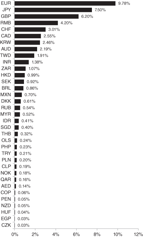
FIGURE 10.2 Currency Exposure as a Percentage of Portfolio Value
TABLE 10.2 Expected Returns, Standard Deviations, and Correlations for Assets and Currencies
 |
Table 10.3 shows the fixed asset class weights as well as the currency‐hedging positions for each of the six strategies presented in Table 10.1. It also shows the standard deviation of each portfolio and its within‐horizon value at risk.
TABLE 10.3 Risk‐Minimizing Hedge Ratios (%)
| No Hedging | Full Hedging | Currency‐Specific Hedging | Cross‐Hedging | Overhedging | Asset Class Reallocation | |
| Hedgeable Foreign Exposure as Percent of Portfolio | 38.1 | 38.1 | 38.1 | 38.1 | 100.0 | 100.0 |
| Total Hedge Positions as Percent of Portfolio | 0.0 | 38.1 | 30.6 | 38.1 | 100.0 | 100.0 |
| Asset Weights | ||||||
| U.S. Equities | 36.8 | 36.8 | 36.8 | 36.8 | 36.8 | 33.1 |
| Foreign Developed Market Equities | 34.5 | 34.5 | 34.5 | 34.5 | 34.5 | 31.3 |
| Emerging Market Equities | 15.8 | 15.8 | 15.8 | 15.8 | 15.8 | 22.0 |
| Treasury Bonds | 0.0 | 0.0 | 0.0 | 0.0 | 0.0 | 10.1 |
| U.S. Corporate Bonds | 8.9 | 8.9 | 8.9 | 8.9 | 8.9 | 1.4 |
| Commodities | 4.0 | 4.0 | 4.0 | 4.0 | 4.0 | 2.1 |
| Cash Equivalents | ||||||
| Hedging Positions | Exposure | Weight | Weight | Weight | Weight | Weight |
| EUR | 9.8 | −9.8 | −9.8 | 0.0 | 0.0 | 0.0 |
| JPY | 7.5 | −7.5 | 0.0 | 0.0 | 0.0 | 0.0 |
| GBP | 6.2 | −6.2 | −6.2 | 0.0 | 0.0 | 0.0 |
| CHF | 3.0 | −3.0 | −3.0 | 0.0 | 0.0 | 0.0 |
| CAD | 2.6 | −2.6 | −2.6 | 0.0 | −27.0 | −25.5 |
| KRW | 2.5 | −2.5 | −2.5 | 0.0 | −21.1 | −21.6 |
| AUD | 2.2 | −2.2 | −2.2 | −31.2 | −28.8 | −28.7 |
| TWD | 1.9 | −1.9 | −1.9 | 0.0 | 0.0 | 0.0 |
| INR | 1.4 | −1.4 | −1.4 | 0.0 | 0.0 | −0.2 |
| ZAR | 1.1 | −1.1 | −1.1 | −6.8 | −23.1 | −24.0 |
| Portfolio | ||||||
| Expected Return | 9.0 | 9.0 | 9.0 | 9.0 | 9.0 | 9.0 |
| Standard Deviation | 16.7 | 14.9 | 14.8 | 12.9 | 9.1 | 8.7 |
| Within‐Horizon Value at Risk* | 30.0 | 26.3 | 25.9 | 21.9 | 13.7 | 12.7 |
*Within‐horizon value at risk is for a three‐year horizon with a 95 percent confidence level expressed as percentage of portfolio value.
Table 10.3 offers a variety of useful insights:
- The fully hedged portfolio has a lower standard deviation than the unhedged portfolio, but not as low as the other hedging strategies, which are less constrained.
- The currency‐specific hedge positions do not reduce standard deviation significantly relative to the fully hedged portfolio. Currency exposures do not introduce meaningful diversification benefits to the portfolio, so the optimal solution is to hedge almost all of the exposure. The sole exception is the Japanese yen, which is not hedged. Table 10.2 reveals that the yen diversifies global equity exposure; it is the only currency that is negatively correlated with the three equity asset classes in the portfolio.
- The cross‐hedging solution uses the Australian dollar and, to a lesser extent, the South African rand to hedge all of the portfolio's currency exposure. Again, Table 10.2 reveals the proximate cause for this selection. The Australian dollar has the highest correlation with foreign developed market equities and emerging market equities of any currency; it therefore offers the most effective hedge.
- The final hedging strategy identifies the risk‐minimizing hedging policy and the optimal asset mix simultaneously. To facilitate comparison, we constrain this solution to have the same expected return as the other portfolios. Also, to ensure that the asset mix is palatable, we control for tracking error relative to the overhedged portfolio.7 Despite these constraints, this solution offers the largest reduction in standard deviation. This is because it lifts a much more impactful constraint: the requirement that the risk‐minimizing currency positions be computed conditioned on a fixed asset mix. In theory, the simultaneous approach always dominates the sequential approach.8 This is true because the ability to hedge the asset classes in advance changes their risk and diversification properties and, hence, their relative weights in an optimal portfolio. For example, in this illustration, the simultaneous solution holds more of the riskiest asset class (emerging market equities) because it is able to offset this risk by hedging highly correlated currencies that are bound together by global growth and commodity prices, such as the Australian dollar and the South African rand. In practice, the simultaneous approach may be impractical. To the extent investors have greater conviction in their estimates of return and risk for asset classes than for currencies, it makes sense to identify the optimal asset mix first.
NONLINEAR HEDGING STRATEGIES
We now evaluate currency‐hedging strategies that employ options. These strategies are classified as nonlinear because the return of the hedged portfolio is a nonlinear function of the hedged currency returns, owing to the asymmetry of option payouts. The primary benefit of options compared to forward contracts is that they preserve the potential for the investor to participate in upside currency returns while hedging the downside. Of course, investors must pay a premium for this protection.
To begin, we consider a straightforward approach in which the investor holds a portfolio of put options—one for each of the 10 major currency exposures in the portfolio. We assume that these options expire every three months, at which time the investor purchases a new set of options. We also assume that the options are at the money and that we purchase enough options to hedge a notional amount equal to the portfolio's explicit exposure to each currency.
To evaluate the performance of the options strategy, we employ Monte Carlo simulation. We choose to simulate rather than backtest the option strategy because a backtest represents only a single pass through history whereas simulation enables us to evaluate a wide range of outcomes in which options expire both in and out of the money. We calibrate these simulations so that the currencies and asset classes have the same expected returns, standard deviations, and correlations as in the linear hedging analysis.
- We construct three‐year, quarterly return paths for asset classes and currencies based on the expected returns, standard deviations, and correlations shown in Table 10.2.
- We calculate and record the following values for each quarter:
- The price of an at‐the‐money option on each currency at the beginning of the quarter.9
- The payoff of each option at the end of the quarter.
- The total return of each option over the quarter, as a percentage of the notional exposure to each currency.
- We combine the option returns with the returns of the unhedged portfolio to evaluate their impact on its returns along the path.
- We repeat this process 10,000 times to generate a large sample of paths.
Table 10.4 shows that the investor pays an average quarterly premium of 0.93 percent to protect the portfolio from currency depreciation. On average, this premium is offset by the payoff at the end of each quarter, which has an average value of 0.92 percent. Because the options are at the money, and we are holding 10 of them, the portfolio of options generates a payoff 93 percent of the time. During quarters when the portfolio has a negative return, the average payoff on the option portfolio is even higher, 1.49 percent. When the foreign asset classes in the portfolio are down, the average payoff and probability of a positive payoff are higher again. However, the incremental change is slight due to the high correlation between the domestic and foreign components of the portfolio.
TABLE 10.4 Hedging Performance with Individual Quarterly Put Options (%)
| Across All Periods | When Portfolio Is Down | When Foreign Assets Are Down | |
| Mean Option Premium as Percent of Portfolio | 0.93 | 0.93 | 0.93 |
| Mean Option Payoff as Percent of Portfolio | 0.92 | 1.49 | 1.50 |
| Probability of Payoff > 0 | 93.39 | 99.76 | 99.86 |
Figure 10.3 shows the impact of the unhedged, linear, and nonlinear hedging strategies on the distribution of currency returns within the portfolio. The asymmetric payoff associated with the put options is visible in the truncated left tail.
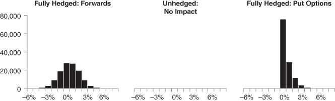
FIGURE 10.3 Impact of Hedging Strategies on Distribution of Portfolio Currency Returns (Quarterly)
In this analysis, we set the notional exposure to each option equal to the explicit notional exposure to the underlying currency. This is the nonlinear equivalent of full hedging. In practice, as is the case with linear hedging, it may be optimal to hedge more or less than this amount of a particular currency exposure. It may also be optimal to combine linear and nonlinear hedging instruments. To identify optimal hedging strategies that account for these complexities, we employ full‐scale optimization as opposed to mean‐variance analysis.10 Full‐scale optimization accounts for the nonnormality of option returns and also enables us to specify a variety of utility functions. We assume that investors wish to protect against currency losses while retaining upside potential; thus, we perform full‐scale optimization using the kinked utility function given in Equation (10.6). (See Chapter 8 for more detail about full‐scale optimization.)
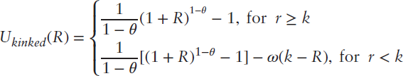
The term ![]() is expected utility,
is expected utility, ![]() is the return of the portfolio,
is the return of the portfolio, ![]() is the location of the kink,
is the location of the kink, ![]() is the curvature, and
is the curvature, and ![]() is the slope. With this utility function, investor satisfaction drops precipitously when returns fall below the kink. (See Chapter 8 for a depiction of a kinked utility function.)
is the slope. With this utility function, investor satisfaction drops precipitously when returns fall below the kink. (See Chapter 8 for a depiction of a kinked utility function.)
When we perform full‐scale optimization, we allow for positions in each option and forward contract to vary between 0 and 100 percent, but we constrain the total positions to be no more than 100 percent. We set curvature, ![]() , and slope,
, and slope, ![]() , equal to 5, and
, equal to 5, and ![]() equal to 0 to reflect aversion to loss. The results of the full‐scale optimization are shown in Table 10.5.11 In addition to the optimal forward and option positions, Table 10.5 shows the following values for unhedged, optimal linear, and optimal nonlinear (full‐scale) hedging strategies:
equal to 0 to reflect aversion to loss. The results of the full‐scale optimization are shown in Table 10.5.11 In addition to the optimal forward and option positions, Table 10.5 shows the following values for unhedged, optimal linear, and optimal nonlinear (full‐scale) hedging strategies:
- Probability of experiencing a quarterly loss
- Average size of quarterly losses
- Within‐horizon value at risk for a one‐year period with 95 percent confidence
TABLE 10.5 Full‐Scale Optimal Hedging Results with Forwards and Options (%)
| Unhedged | Linear Optimal (Overhedging) | Full‐Scale Optimal with 0 Percent Threshold | |
| Unhedged portfolio | 100.0 | 100.0 | 100.0 |
| Forward Positions | |||
| EUR | 0.0 | 0.0 | 0.0 |
| JPY | 0.0 | 0.0 | 0.0 |
| GBP | 0.0 | 0.0 | 0.0 |
| CHF | 0.0 | 0.0 | 0.0 |
| CAD | 0.0 | −27.0 | −34.3 |
| KRW | 0.0 | −21.1 | −28.8 |
| AUD | 0.0 | −28.8 | −11.9 |
| TWD | 0.0 | 0.0 | 0.0 |
| INR | 0.0 | 0.0 | 0.0 |
| ZAR | 0.0 | −23.1 | −25.0 |
| Put Option Positions | |||
| EUR | 0.0 | 0.0 | 0.0 |
| JPY | 0.0 | 0.0 | 0.0 |
| GBP | 0.0 | 0.0 | 29.9 |
| CHF | 0.0 | 0.0 | 0.0 |
| CAD | 0.0 | 0.0 | 10.2 |
| KRW | 0.0 | 0.0 | 0.0 |
| AUD | 0.0 | 0.0 | 0.0 |
| TWD | 0.0 | 0.0 | 9.9 |
| INR | 0.0 | 0.0 | 33.9 |
| ZAR | 0.0 | 0.0 | 0.0 |
| Probability of Return < 0 Percent | 42% | 35% | 35% |
| Average Return < 0 Percent | −6.7 | −3.1 | −2.8 |
| Within‐Horizon Value at Risk* | −23.5 | −10.3 | −9.5 |
*Within‐horizon VaR is for a one‐year horizon with a 95% confidence level and quarterly monitoring.
The optimal linear solution, which is the overhedging strategy repeated from Table 10.3, reduces the probability and average magnitude of losses relative to the unhedged portfolio. However, the full‐scale solution, which accounts for the nonnormality of option returns as well as the investor's preference for upside versus downside returns, shows additional improvement in these metrics. It is notable from these results that the nonlinear solution uses options to hedge the British pound, Taiwanese dollar, and Indian rupee, which are left unhedged in the linear solution. Evidently, hedging these exposures with forward contracts does not reduce the portfolio's standard deviation, but hedging them with put options reduces the likelihood and magnitude of losses.
Investors may also wish to consider the following nonlinear hedging strategies. We can also measure their benefits and costs with simulation.
- Basket option. This strategy purchases a single option to hedge the portfolio's collective currency exposure. A basket option is cheaper than a portfolio of put options, because diversification among the currencies reduces the volatility of the basket. However, it also reduces the average payout.
- Foreign asset contingent option. This strategy purchases a basket option that pays off only when two outcomes occur simultaneously: a loss in the foreign asset component of the portfolio and a loss in the collective currency basket. In other words, this option provides protection only in periods when both currencies and foreign assets are down. This strategy may appeal to an investor who is able to tolerate adverse currency outcomes when they are offset by gains in the underlying assets. Because it offers less protection overall, this strategy is less expensive than a basket option.
- Total portfolio contingent option. This strategy is equivalent to the one described above; however, the first contingency is linked to the entire portfolio rather than the foreign asset component.
ECONOMIC INTUITION
We have shown that the optimal hedging strategy rarely, if ever, hedges all currencies in the same proportion. This result is driven by the empirical fact that some currencies are more correlated with assets than others. Likewise, investors in certain countries should hedge more than investors in other countries. Some may wonder whether these results are based on sound economic intuition or merely represent statistical properties that are unlikely to persist in the future. We argue that correlations differ for sound economic reasons. Each currency is inexorably linked to its underlying economy and varies with the unique set of macroeconomic factors that influence that economy. For example, the Swiss franc is often viewed as a safe‐haven currency that investors buy during market crises. As a result, it tends to be less correlated with global equity markets, particularly during turbulent periods. Therefore, most investors should not hedge the Swiss franc because it introduces favorable diversification to their portfolio. Swiss investors, on the other hand, may want to hedge more than investors in other countries because foreign currencies, denominated in Swiss francs, tend to have higher correlations with global equity markets.
This intuition may sound plausible, but to formulate a hedging policy, we must have confidence that these relationships will persist in the future. This chapter presents in‐sample results. That is, we compute the hedge ratios and evaluate their performance using the same sample of returns (or simulated returns drawn from the same distribution). In practice, of course, realized results differ from expectations, and the performance of these strategies will depend on the persistence of the inputs from one period to the next. Kinlaw and Kritzman (2009) present an extensive empirical study of both equity and multi‐asset class portfolios. They conclude that currency standard deviations and correlations are reasonably persistent through time. The economic rationale described above, combined with the empirical persistence of these relationships, should give investors some degree of comfort that history serves as a reasonable guide to the future behavior of currencies.
REFERENCES
- W. Chen, M. Kritzman, and D. Turkington. 2015. “Alternative Currency Hedging Strategies with Known Covariances,” Journal of Investment Management, Vol. 13, No. 2 (Second Quarter).
- G. Chow. 1995. “Portfolio Selection Based on Return, Risk, and Relative Performance,” Financial Analysts Journal, Vol. 51, No. 2 (January/February).
- M. Adler and B. Prasad. 1992. “On Universal Currency Hedges,” Journal of Financial and Quantitative Analysis, 27(1)
- F. Black. 1989. “Universal Hedging: Optimizing Currency Risk and Reward in International Equity Portfolios, Financial Analysts Journal, (July/August)
- J. Cremers, M. Kritzman, and S. Page. 2005. “Optimal Hedge Fund Allocations,” Journal of Portfolio Management, Vol. 31, No. 3 (Spring).
- G. Gardner and T. Wuilloud. 1995. “Currency Risk in International Portfolios: How Satisfying is Optimal Hedging?” Journal of Portfolio Management, Vol. 21, No. 3 (Spring).
- M. Garman and S. Kohlhagen. 1983. “Foreign Currency Option Values,” Journal of International Money and Finance, Vol. 2, No. 3 (December).
- P. Jorian. 1994. “Mean Variance Analysis of Currency Overlays,” Financial Analysts Journal, Vol. 50, No. 3 (May/June).
- W. Kinlaw and M. Kritzman. 2009. “Optimal Currency Hedging In and Out of Sample,” Journal of Asset Management, Vol. 10, No. 1 (April).
- J. M. Schmittmann. 2010. “Currency Hedging for International Portfolios,” IMF Working Paper (June).
- J. Siegel. 1975. “Risk, Interest Rates, and the Forward Exchange,” Quarterly Journal of Economics, February 1975.