
CHAPTER 18
Statistical and Theoretical Concepts
This chapter provides a brief introduction to concepts in statistics and portfolio theory. We include a fair amount of math, but we do our best to avoid excessive complexity. Our intent is to establish a sufficient foundation for this book that is reasonably clear, but this review is by no means comprehensive. We therefore include references to other sources that provide a more thorough and technical explanation of these topics.
DISCRETE AND CONTINUOUS RETURNS
We define the discrete return ![]() for an asset from time
for an asset from time ![]() to
to ![]() as the change in price over some period plus any income generated, all divided by the price at the beginning of the period:
as the change in price over some period plus any income generated, all divided by the price at the beginning of the period:

Next, we denote the log return of the asset using a lowercase ![]() :
:
Here ![]() is the natural logarithm function. The log return represents the continuous rate of return for the period. In other words, it is the instantaneous rate of return that, if compounded continuously, would match the asset's realized total return. The natural logarithm of
is the natural logarithm function. The log return represents the continuous rate of return for the period. In other words, it is the instantaneous rate of return that, if compounded continuously, would match the asset's realized total return. The natural logarithm of ![]() is simply the exponent to which the special number e, which is approximately equal to 2.71828, is raised to yield
is simply the exponent to which the special number e, which is approximately equal to 2.71828, is raised to yield ![]() . Therefore, the logarithm is the inverse of the exponential function, which we denote as
. Therefore, the logarithm is the inverse of the exponential function, which we denote as ![]() , or equivalently
, or equivalently ![]() . To express the discrete return
. To express the discrete return ![]() , we reverse Equation (18.2), as shown:
, we reverse Equation (18.2), as shown:
Together, the exponential and logarithmic functions relate continuously compounded growth rates to returns that occur over discrete time intervals. Discrete time is observable and measurable, whereas continuous time is not. The returns we compute from data are in discrete units, but we often use continuous returns in analysis because they have important properties, which we discuss later.
ARITHMETIC AND GEOMETRIC AVERAGE RETURNS
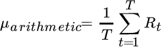
The arithmetic average return for an asset (also called the mean return) is one of the most obvious and informative summary statistics. Suppose an asset is worth $100 initially, appreciates to $125 after one year, and falls back to $100 after the second year. The discrete annual returns are +25 percent and –20 percent. The arithmetic average of the discrete returns is equal to the sum of the two returns divided by 2: [![]() . More generally, for
. More generally, for ![]() time periods the arithmetic average is:
time periods the arithmetic average is:
The 2.5 percent average return we calculated for our hypothetical asset presents a conundrum. It implies that the asset gained value on average, yet it was worth the same amount at the end of two periods as it was at the beginning. This apparent contradiction occurs because the arithmetic average of discrete returns ignores the effect of compounding. For this reason, the geometric average, which accounts for compounding, is more appropriate for summarizing past investment performance. In this example, the geometric average of discrete returns is equal to ![]() , which agrees with the cumulative growth of the asset. For
, which agrees with the cumulative growth of the asset. For ![]() time periods, the geometric average is given by:
time periods, the geometric average is given by:

We also arrive at the geometric average by converting the discrete returns to continuous returns, taking the arithmetic mean of the resulting continuous returns, and then converting the result back to a discrete return:
Stated generally:

Given that the arithmetic average ignores that returns compound over multiple periods, why should we bother with it? It turns out that the arithmetic average has a very important advantage in a portfolio context. As we discuss in Chapter 2, the arithmetic average of a weighted sum of variables is equal to the sum of the arithmetic averages of the variables themselves. This relationship does not hold for the geometric average. In order to arrive at the average return of a portfolio from the averages of the assets within it, we must use arithmetic averages.
STANDARD DEVIATION
Average return tells us nothing about the variation in returns over time. To analyze risk, we must look at deviations from the average. The larger an asset's deviations from its average return—in either a positive or a negative direction—the more risky it is. We use a statistic called standard deviation, ![]() , to summarize the variability of an asset's returns, and we calculate it as the square root of the average of squared deviations from the mean:
, to summarize the variability of an asset's returns, and we calculate it as the square root of the average of squared deviations from the mean:

We must square the deviations before we average them. Otherwise, the average would equal zero. By taking the square root of the average squared deviations, we convert this measure back to the same units as the original returns. Standard deviation is a summary measure because the squared deviations are averaged together. As we will see later, there are nuances in the actual deviations that are not captured by standard deviation.
The average of the squared deviations is called the variance. We often use the variance when we perform mathematical operations, but its square root, standard deviation, is a more intuitive description of risk, and it has useful properties, which we discuss later on.
Equation (18.9) shows what is known as the population parameter for standard deviation because it multiplies the sum of the deviations by ![]() . It turns out that this estimate of standard deviation is biased. It underestimates the true standard deviation because it implicitly assumes we know the true mean return for the asset, which we do not. We solve this problem by using
. It turns out that this estimate of standard deviation is biased. It underestimates the true standard deviation because it implicitly assumes we know the true mean return for the asset, which we do not. We solve this problem by using ![]() instead. The resulting estimate is called the sample statistic. We use the sample statistic for the empirical analysis in this book, but we describe risk statistics in terms of the population parameters in this section of this chapter for convenience. The distinction is not very important in practice, especially when there are a large number of observations.
instead. The resulting estimate is called the sample statistic. We use the sample statistic for the empirical analysis in this book, but we describe risk statistics in terms of the population parameters in this section of this chapter for convenience. The distinction is not very important in practice, especially when there are a large number of observations.
CORRELATION
When two assets are combined, the standard deviation of the combination depends not only on each asset's standard deviation but also on the degree to which the assets move together or in opposition. The correlation between two assets is a statistical measure of their comovement. Correlations can be as low as ![]() 1, which indicates complete opposite movement, and as high as +1, which indicates they move in perfect unison. A correlation of 0 suggests that assets are uncorrelated with one another. Correlations are computed by multiplying each deviation for asset
1, which indicates complete opposite movement, and as high as +1, which indicates they move in perfect unison. A correlation of 0 suggests that assets are uncorrelated with one another. Correlations are computed by multiplying each deviation for asset ![]() with the deviation for asset
with the deviation for asset ![]() for the same period, averaging these products across all periods, and dividing the result by the product of the standard deviations of both variables to normalize the measure:
for the same period, averaging these products across all periods, and dividing the result by the product of the standard deviations of both variables to normalize the measure:
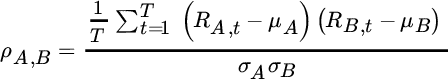
Correlation, therefore, captures the degree to which deviations align for two assets, on average. Just as there are aspects of risk that are not captured by standard deviation, there are aspects of comovement that are not captured by correlation. Nevertheless, correlations are very useful for summarizing the similarities or differences in the way asset returns interact.
COVARIANCE
The covariance between two assets equals their correlation multiplied by each of their standard deviations. It reflects the tendency of assets to move together as well as the average size of their movements. The covariance between two assets ![]() and
and ![]() over
over ![]() periods is also equal to the numerator from Equation (18.10):
periods is also equal to the numerator from Equation (18.10):

Variance is a special case of covariance. It is the covariance of an asset with itself. A covariance matrix, which contains the variances of every asset and the covariances between every pair of assets, under many conditions, provides an excellent summary of risk for any universe of ![]() assets. The covariance matrix, denoted in matrix notation as
assets. The covariance matrix, denoted in matrix notation as ![]() , is an
, is an ![]() matrix in which the element in the
matrix in which the element in the ![]() ‐th row and
‐th row and ![]() ‐th column contains the covariance between the
‐th column contains the covariance between the ![]() ‐th and
‐th and ![]() ‐th assets. Diagonal entries are variances. A covariance matrix is always symmetric because its entries for
‐th assets. Diagonal entries are variances. A covariance matrix is always symmetric because its entries for ![]() and
and ![]() ,
, ![]() are identical.
are identical.
COVARIANCE INVERTIBILITY
Portfolio applications require covariance matrices to be invertible. Essentially, this means that it must be possible to derive a matrix called the covariance matrix inverse, which, when multiplied by the covariance matrix, returns an identity matrix with 1s along its diagonal and 0s everywhere else. In very general terms, we can think of the covariance matrix as a measure of risk, and its inverse as a matrix that neutralizes that risk. The inverse covariance matrix is essential for portfolio optimization, as we discuss in Chapter 2.
In order for a covariance matrix to be invertible, it must be internally consistent. Imagine being presented with a blank 10‐by‐10 grid and asked to fill in values for a covariance matrix. The challenge might resemble a giant Sudoku problem in which prior choices constrain future possibilities. If asset A is highly correlated to asset B, and asset B is highly correlated to asset C, then asset A is very likely to be correlated to asset C. With a large web of cross‐asset relationships, it is not hard to concoct covariance matrices that imply impossible asset interactions.
Luckily, when we use a sufficient number of returns to estimate a covariance matrix, it is guaranteed to be invertible. We have a problem only when we have more assets ![]() in our universe than we have independent historical returns
in our universe than we have independent historical returns ![]() on which to estimate the covariance matrix, or if we override empirical covariances with our views. To be invertible, a matrix must be positive‐semi‐definite, which means that any set of asset weights is guaranteed to produce a portfolio with nonnegative variance. Negative variance cannot exist, so any covariance matrix that implies negative variance is flawed. We are more likely to encounter a problem when the number of assets is large, such as in security selection as opposed to asset allocation. But if the need arises, we can “correct” the covariance matrix using a technique that involves Principal Components Analysis.
on which to estimate the covariance matrix, or if we override empirical covariances with our views. To be invertible, a matrix must be positive‐semi‐definite, which means that any set of asset weights is guaranteed to produce a portfolio with nonnegative variance. Negative variance cannot exist, so any covariance matrix that implies negative variance is flawed. We are more likely to encounter a problem when the number of assets is large, such as in security selection as opposed to asset allocation. But if the need arises, we can “correct” the covariance matrix using a technique that involves Principal Components Analysis.
Principal Components Analysis is a useful technique for many applications. It decomposes a covariance matrix into a matrix, ![]() , composed of eigenvectors in each column, and a diagonal matrix of eigenvalues,
, composed of eigenvectors in each column, and a diagonal matrix of eigenvalues, ![]() :
:
Eigenvectors are completely orthogonal to each other, and they span the entire set of asset returns. Though the elements in each eigenvector do not sum to 1 (their squared values sum to 1), we interpret an eigenvector as a set of portfolio weights. The top eigenvector, also called the top principal component, is the portfolio with the highest possible variance. It explains more variation in the returns than any other vector. Its corresponding eigenvalue represents its variance. All subsequent eigenvectors are completely uncorrelated to those that came before, and they explain successively lower amounts of variation in the asset returns.
A matrix is positive‐semi‐definite if all of its eigenvalues are greater than or equal to zero. An eigenvalue equal to zero implies there is a combination of assets that yields zero risk, or, put differently, that there are two distinct portfolios with exactly opposite return behavior. The presence of redundant portfolio combinations may pose a challenge to portfolio construction, because there may not be a unique optimal portfolio. The existence of a negative eigenvalue is far more troubling, because it implies that we can create a portfolio with negative risk. Obviously, that is impossible. The covariance matrix is inconsistent and does not represent feasible relationships among assets.
To render a matrix positive‐semi‐definite, we replace offending eigenvalues with zeros and reconstruct the covariance matrix using this new assumption. To render it positive‐definite, we substitute small positive values. Problematic eigenvalues tend to be small to begin with, so these adjustments have a relatively minor effect on the matrix. Nevertheless, we should approach these adjustments with care.
MAXIMUM LIKELIHOOD ESTIMATION
In practice, the amount of historical returns available for each asset class may differ. Nonequal history lengths present a choice. We could use the common sample, and discard the extra returns for the asset classes with longer histories. Or we could restrict our investment universe to include only asset classes with long return histories, and thereby forgo the potential benefits of including asset classes with shorter histories. A third, and perhaps more appealing, option is to make use of all available returns by using Maximum Likelihood Estimation (MLE).
We can use MLE for means as well as covariances. The MLE method solves for the parameter that is most likely to have produced the observed returns. It is a general technique used throughout statistics, and it accommodates missing returns easily. We do not describe the implementation of MLE algorithms in detail, but the techniques are well documented elsewhere and are available in common statistical software packages.
Nonetheless, here's an intuitive description of MLE. Suppose we have an asset class with a long history of returns and one with a short history. The short history is common to both asset classes. Therefore, in order to estimate a covariance that pertains to both asset classes for the long history, we incorporate information about the interaction of the two asset classes during the short history that is common to both of them. We use this information, along with the returns of the asset class with the long history that preceded the short history, to arrive at a covariance that is statistically the most likely value. This approach produces estimates that are statistically consistent and likely to be positive‐semi‐definite. We can also use the MLE estimates to “backfill” missing historical returns conditioned on the returns available at each point in time. Backfilling procedures are useful when we require a full empirical sample.1
MAPPING HIGH‐FREQUENCY STATISTICS ONTO LOW‐FREQUENCY STATISTICS
We have assumed so far that means and covariances pertain to the time interval over which historical returns are measured. However, we often use monthly returns to estimate the properties of annual returns, for example. It turns out that mapping statistics estimated from high‐frequency observations onto low‐frequency statistics is not a trivial exercise. Let's assume for now that returns are independent and identically distributed (IID) across time. In other words, they do not trend or mean‐revert, and their distribution remains stable. We relax this important assumption in Chapter 13, but doing so is beyond the scope of our current discussion. Even for IID returns, though, something interesting happens when we consider the impact of compounding. As we measure compound returns over longer and longer periods, the distribution of returns changes shape. Compound returns cannot be less than ![]() 100 percent, but they can grow arbitrarily large. Overall, losses are compressed by compounding, and gains are amplified. The longer the time horizon, and the more volatile the assets, the more dramatic this downside compression and upside extension will be.
100 percent, but they can grow arbitrarily large. Overall, losses are compressed by compounding, and gains are amplified. The longer the time horizon, and the more volatile the assets, the more dramatic this downside compression and upside extension will be.
We solve this problem by converting statistics into their continuous counterparts (described earlier in this chapter), applying the time horizon adjustment to continuous returns, and translating the result back to discrete returns. It is indeed true that average return scales linearly with time for IID continuous returns. Likewise, standard deviations scale with the square root of time under these conditions.
Here is how we adjust for time horizon. We begin with discrete high‐frequency returns (monthly or daily, not milliseconds), and we convert them to continuous units using the following formulas:
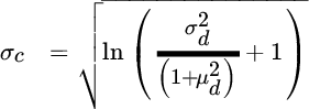

Next, we multiply ![]() by the frequency we desire, such as 12 to convert from monthly to annual units, and we multiply
by the frequency we desire, such as 12 to convert from monthly to annual units, and we multiply ![]() by the square root of that frequency. These statistics now apply to the longer horizon, but they are still in continuous units. We convert them back to discrete units using the following formulas:
by the square root of that frequency. These statistics now apply to the longer horizon, but they are still in continuous units. We convert them back to discrete units using the following formulas:
PORTFOLIOS
Assume that we create a portfolio with weights ![]() that sum to 1 across
that sum to 1 across ![]() assets and we rebalance the portfolio weights at the beginning of each period. The discrete return of portfolio
assets and we rebalance the portfolio weights at the beginning of each period. The discrete return of portfolio ![]() from year
from year ![]() to
to ![]() is a simple weighted average of the discrete returns for the assets:
is a simple weighted average of the discrete returns for the assets:
Here ![]() is the discrete return of asset
is the discrete return of asset ![]() . The mean return for the portfolio is then:
. The mean return for the portfolio is then:
This relationship holds because the expected value of a sum of variables is equal to the sum of the variables' expected value. We compute the variance of an ![]() ‐asset portfolio as a sum across every pair of assets:
‐asset portfolio as a sum across every pair of assets:
Matrix algebra offers more succinct notation for portfolio arithmetic. Throughout this book, we indicate vectors and matrices in formulas using bold font. We assume vectors to be column vectors unless stated otherwise. For a vector ![]() of
of ![]() weights across assets, a vector
weights across assets, a vector ![]() of their means, an
of their means, an ![]() ×
× ![]() covariance matrix
covariance matrix ![]() , and using the symbol
, and using the symbol ![]() to denote the matrix transpose, we express the portfolio's mean and variance as:
to denote the matrix transpose, we express the portfolio's mean and variance as:
PROBABILITY DISTRIBUTIONS
A probability distribution defines a random variable's possible values and how likely they are to occur. Discrete distributions (not to be confused with discrete returns) allow a fixed set of values and assign a probability between 0 and 1 to each outcome such that the sum of the probabilities equals 1. Specifically, we say that a random variable ![]() takes on one of
takes on one of ![]() values
values ![]() with probability
with probability ![]() .
.
It is often more useful to study variables that take on any of the infinite values in some range. In this case, the distribution is continuous and is defined as a probability density function (PDF). Strictly speaking, the probability that the variable takes on any particular value, such as 0.013425, is zero because point values are infinitely small and there are infinitely many of them. But we can easily calculate the probability that a variable will take on a value within a defined range using an integral to capture the area under the curve. If ![]() has a continuous probability distribution with probability density function
has a continuous probability distribution with probability density function ![]() , its integral, which measures the area underneath its curve, equals one when summed across all possible values:
, its integral, which measures the area underneath its curve, equals one when summed across all possible values:

THE CENTRAL LIMIT THEOREM
The Central Limit Theorem is a profound result in statistics. It states that the sum (or average) of a large number of random variables is approximately normally distributed, as long as the underlying variables are independent and identically distributed and have finite variance. This result is powerful because the normal distribution is described entirely by its mean and variance, whereas the component distributions might be far more complicated. Given that many processes in nature, and in finance, involve outcomes that are aggregations of many other random events, we should expect to see many variables with distributions close to normal. And indeed we do.
THE NORMAL DISTRIBUTION
The normal (or Gaussian) distribution looks like a bell‐shaped curve. It is centered around the mean, with tails that decay symmetrically on both sides. The normal distribution has many attractive properties:
 It characterizes the sum of large numbers of other variables, regardless of their distribution, due to the Central Limit Theorem.
- It is fully described by its mean and variance. Fitting a normal distribution to data requires estimating only two parameters.
- The sum of normally distributed variables is also normally distributed.
Whereas a single‐variable normal distribution is described by its mean and variance, a multivariate normal distribution is described by its mean vector and covariance matrix.
HIGHER MOMENTS
The statistics of mean and variance are special cases of a more general way to describe distributions, known as moments. It is easier to conceptualize what are known as “central” moments of a distribution. Each moment is, quite simply, the average of all deviations from the mean raised to a specified power. The first central moment is the (signed) average of each return minus the mean, which is always equal to zero. The second central moment is the variance, which we have already discussed at length in this chapter. Subsequent moments are often termed “higher moments,” and they measure departures from normality. The third central moment measures asymmetry. It is often normalized by dividing by the standard deviation cubed, and is called skewness. If larger returns are disproportionately positive, the distribution will be positively skewed, and the opposite will be true for negative returns. The fourth central moment divided by standard deviation raised to the fourth power is called kurtosis, and it is often evaluated in relation to the kurtosis of a normal distribution. Distributions with larger kurtosis than a normal distribution (which has kurtosis equal to 3) are said to be leptokurtic; they have larger probabilities of extreme positive and negative outcomes than a normal distribution. Those that have lower kurtosis than a normal distribution are platykurtic, with greater probability of moderate outcomes. We can proceed in this fashion indefinitely, computing higher and higher moments, but the first four are usually adequate to describe the salient features of asset returns.
THE LOGNORMAL DISTRIBUTION
The effect of compounding introduces skewness to returns. Consider, for example, a bet that either gains 1 percent or loses 1 percent with equal probability. If such a bet is taken once per month, the distribution of monthly returns will be symmetric. However, the compound return of two successive losses is ![]() 1.99 percent, while the equally likely return of successive gains is 2.01 percent. After five years, the spread widens to 81.67 percent for 60 gains and only
1.99 percent, while the equally likely return of successive gains is 2.01 percent. After five years, the spread widens to 81.67 percent for 60 gains and only ![]() 45.28 percent for 60 losses. In fact, the increase in wealth associated with any sequence of compound gains is larger than the decrease in wealth for an equal‐size, but opposite, series of compound losses. The distribution of returns has positive skewness. The lognormal distribution is positively skewed and captures this behavior. If we assume an asset's instantaneous rate of growth is normally distributed, then its discrete returns are lognormally distributed.
45.28 percent for 60 losses. In fact, the increase in wealth associated with any sequence of compound gains is larger than the decrease in wealth for an equal‐size, but opposite, series of compound losses. The distribution of returns has positive skewness. The lognormal distribution is positively skewed and captures this behavior. If we assume an asset's instantaneous rate of growth is normally distributed, then its discrete returns are lognormally distributed.
ELLIPTICAL DISTRIBUTIONS
Elliptical distributions are defined by the fact that the returns that lie along a given ellipsoid must be equally likely. This implies that the probability density function depends on ![]() only through its covariance‐adjusted distance from its mean. Therefore, if
only through its covariance‐adjusted distance from its mean. Therefore, if ![]() is a column vector random variable,
is a column vector random variable, ![]() is a column vector representing the mean of
is a column vector representing the mean of ![]() , and
, and ![]() is the covariance matrix for
is the covariance matrix for ![]() , the density is proportional to some function of the covariance‐adjusted distance:
, the density is proportional to some function of the covariance‐adjusted distance:
Based on this definition, we can make the following observations:
- Elliptical distributions are symmetric.
- The multivariate normal distribution is an elliptical distribution.
- Elliptical distributions can have “fatter tails” than a normal distribution. However, the shape of the tails must be consistent across assets.
PROBABILITY OF LOSS
Assume that a portfolio has a discrete expected return ![]() and standard deviation
and standard deviation ![]() over some specified time period, and that we want to measure the probability that ending wealth will fall below
over some specified time period, and that we want to measure the probability that ending wealth will fall below ![]() . For long horizons, the impact of compounding could be substantial, so we should assume that the portfolio's discrete returns,
. For long horizons, the impact of compounding could be substantial, so we should assume that the portfolio's discrete returns, ![]() , follow a lognormal distribution. The loss threshold in continuous return units is
, follow a lognormal distribution. The loss threshold in continuous return units is ![]() , and we compute the continuous counterparts for the portfolio's expected return and standard deviation using Equations (18.13) and (18.14). Because
, and we compute the continuous counterparts for the portfolio's expected return and standard deviation using Equations (18.13) and (18.14). Because ![]() and
and ![]() describe a normal distribution in continuous units, we estimate the probability of loss by applying the cumulative normal distribution function
describe a normal distribution in continuous units, we estimate the probability of loss by applying the cumulative normal distribution function ![]() as follows:
as follows:

VALUE AT RISK
Value at risk is the inverse of probability of loss. It represents the worst outcome we should expect with a given level of confidence. We derive value at risk by solving for ![]() in Equation (18.25), where
in Equation (18.25), where ![]() is the inverse cumulative normal distribution function:
is the inverse cumulative normal distribution function:
UTILITY THEORY
A utility function ![]() expresses the satisfaction an investor receives from any specified level of wealth
expresses the satisfaction an investor receives from any specified level of wealth ![]() . A utility function may take many forms, but a plausible utility function for a rational investor meets at least two criteria:
. A utility function may take many forms, but a plausible utility function for a rational investor meets at least two criteria:
- It is upward sloping, which means that the investor prefers more wealth to less.
- It is concave, which means that the investor's incremental utility from a gain is less than the investor's incremental disutility from an equal‐size loss.
This second point implies aversion to risk. Investors with more dramatic curvature in utility are inclined to invest more cautiously, while those with a relatively flatter utility function are inclined to invest more aggressively.
SAMPLE UTILITY FUNCTIONS
For ease of interpretation, we express utility in terms of the discrete period's return  , which is simply the percentage of change in wealth. Let us first consider the class of “power utility” functions, which takes the following form:
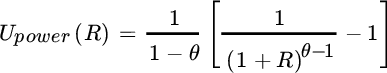
A given return is raised to the power ![]() , where
, where ![]() . Larger values for
. Larger values for ![]() imply greater risk aversion. Investors who are characterized by this class of utility functions are said to have “constant relative risk aversion.” This means that they prefer to maintain the same exposure to risky assets regardless of their wealth. In the limit, as
imply greater risk aversion. Investors who are characterized by this class of utility functions are said to have “constant relative risk aversion.” This means that they prefer to maintain the same exposure to risky assets regardless of their wealth. In the limit, as ![]() approaches
approaches ![]() , power utility becomes the commonly used “log‐wealth” utility function:
, power utility becomes the commonly used “log‐wealth” utility function:
ALTERNATIVE UTILITY FUNCTIONS
Some investors are strongly averse to losses that breach a particular threshold because it may cause their circumstances to change abruptly. They are characterized by a “kinked” utility function (see Figure 18.1), which is equal to power utility (or, alternatively, log utility) plus an additional penalty of ![]() for each unit of loss below a threshold,
for each unit of loss below a threshold, ![]() :
:

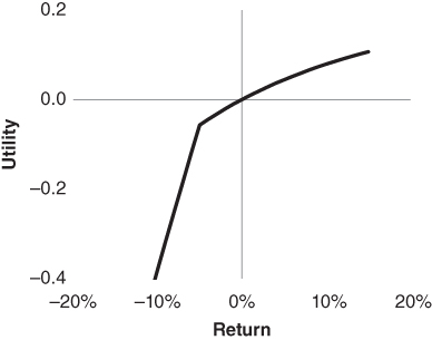
FIGURE 18.1 Kinked Utility Function
Behavioral economists have found that even though most people exhibit risk aversion with respect to gains in wealth, many display risk‐seeking behavior when they face losses. Instead of accepting a guaranteed loss of some amount, these people prefer to gamble between a smaller loss and a larger loss in the hope that they can avoid some pain if they are lucky. An S‐shaped utility curve characterizes this preference (see Figure 18.2).
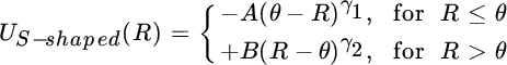

FIGURE 18.2 S‐Shaped Utility Function
While we believe that these particular utility functions describe a relevant cross section of investor preferences, they are by no means exhaustive. Many other utility functions have been proposed in the literature. We leave it to the reader to apply the concepts in this book to other specifications of investor utility.
EXPECTED UTILITY
We can use a utility function to describe an investor's relative preference among risky bets. For example, suppose that bet ![]() offers a 50 percent chance of a 20 percent gain and a 50 percent chance of a 10 percent loss. Bet
offers a 50 percent chance of a 20 percent gain and a 50 percent chance of a 10 percent loss. Bet ![]() offers a 50 percent chance of a 30 percent gain and a 50 percent chance of a 20 percent loss. Expected utility is the probability‐weighted utility for each bet. Assuming log utility, the utility of each bet is:
offers a 50 percent chance of a 30 percent gain and a 50 percent chance of a 20 percent loss. Expected utility is the probability‐weighted utility for each bet. Assuming log utility, the utility of each bet is:
A log‐wealth investor would prefer bet ![]() in this example, given its higher expected utility.
in this example, given its higher expected utility.
CERTAINTY EQUIVALENTS
If we know an investor's expected utility for a risky bet, we can compute the size of a single risk‐free return that yields identical utility. This quantity is called the “certainty equivalent.” Given a particular utility function, an investor is indifferent to the uncertain outcome of the risky bet and the guaranteed certainty‐equivalent return. Recalling our simple example, we use the exponential function, which is the inverse of the logarithm, to calculate the certainty equivalents for bets ![]() and
and ![]() :
:
MEAN‐VARIANCE ANALYSIS FOR MORE THAN TWO ASSETS
For a universe of ![]() assets, we express mean‐variance expected utility as a function of a column vector of portfolio weights
assets, we express mean‐variance expected utility as a function of a column vector of portfolio weights ![]() , a column vector of expected returns
, a column vector of expected returns ![]() , and an
, and an ![]() x
x![]() covariance matrix
covariance matrix ![]() :
:
To solve for the weights that maximize expected utility, we take its derivative with respect to the weight vector and set the derivative equal to zero:
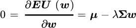
Rearranging this expression, we find that the optimal weights are:
These optimal weights are not subject to any constraints; they can be arbitrarily large positive or negative numbers and can sum to any amount. In this context, the investor's risk aversion changes the amount allocated to the optimal mix, but it does not change the relative allocation across assets. Due to its mathematical simplicity, this unconstrained solution serves as a useful reference. These portfolios may require shorting and leverage, but they could be investable assuming we borrow to account for any funding shortfall (if the sum of the weights exceeds 100 percent of available capital) or invest excess proceeds at the risk‐free rate (if the sum of the weights falls below 100 percent of available capital).
It is possible to derive analytical expressions for optimal weights subject to constraints (such as the analytical example presented in Chapter 5), but we will not delve into these mathematical solutions in detail. Many other books describe them thoroughly. Instead, we simply note that quadratic programming algorithms, which are easily accessible in popular software packages and programming languages, solve for mean‐variance optimal weights in the presence of upper and lower bounds on each individual asset weight as well as equality and inequality constraints for sums of asset weights. (In Chapter 2 we review two specific methods of solving for optimal weights in the presence of constraints.)
EQUIVALENCE OF MEAN‐VARIANCE ANALYSIS AND EXPECTED UTILITY MAXIMIZATION
Mean‐variance optimization is equivalent to maximizing expected utility if either of two conditions holds:
- Investor utility is a quadratic function.
- Asset returns are elliptically distributed.
To understand the first point on an intuitive level, note that the quadratic utility function contains a linear term, which is a simple multiple of return, and a quadratic term, which is a multiple of return squared. Expected utility averages utility across a distribution of return outcomes, so it includes an average of the return and an average of the squared return. These two averages equal the mean and the variance, respectively, so we can completely describe utility in terms of a portfolio's mean and variance. As long as we restrict our attention to the portion of a quadratic utility curve in which utility is increasing, we know that the curve implies risk aversion; therefore, the portfolio that minimizes variance for a given level of return must also maximize expected utility (for some level of risk aversion).
Importantly, a portfolio composed of elliptical assets is itself elliptically distributed. The symmetry of the portfolio distribution is enough to guarantee that for any plausible utility function that is upward sloping and concave, we can obtain the expected utility‐maximizing portfolio using mean‐variance analysis.
If asset returns are nonelliptical and investor utility is not quadratic, then mean‐variance analysis is not strictly equivalent to expected utility maximization. However, it usually provides a very good approximation to the true expected utility‐maximizing result.
MONTE CARLO SIMULATION
In some instances, simulation techniques are used to produce more reliable estimates of exposure to loss than the formulas we described earlier. For example, when lognormally distributed returns are combined in a portfolio, the portfolio itself does not have a lognormal distribution. The shape of the lognormal distribution varies across asset classes depending on the asset classes' expected growth rates and their volatility. Short positions cause an even more dramatic difference in volatility because their returns are negatively skewed due to compounding, whereas the returns to long positions are positively skewed. In these circumstances, we should simulate random normal return samples for the asset classes in continuous units, apply the effect of compounding, consolidate returns into a single portfolio, and compute risk metrics for the resulting portfolio distribution. In particular, we perform the following steps:
- Draw one set of random returns from a multivariate normal distribution with a continuous mean and covariance equal to that of the asset classes.
- Convert each continuous return to its discrete equivalent by raising e to the power of the continuous return and subtracting 1.
- Multiply the discrete asset class returns by the portfolio weights to compute the portfolio's return.
- Repeat steps 1 through 3 to produce a sample of 1,000 portfolio returns.
- Count the percentage of simulated returns that fall below a given threshold to estimate probability of loss, or sort returns according to their size and identify the return of the 50th most negative return (given a sample of 1,000) as the five percentile value‐at‐risk.
BOOTSTRAP SIMULATION
Bootstrap simulation is similar to Monte Carlo simulation, but the simulated observations are selected from an empirical distribution instead of a theoretical one like the lognormal distribution. For example, we could generate thousands of hypothetical one‐year returns by repeatedly sampling a different collection of 12 months from history and combining them. In doing so, we preserve the empirical distribution of the asset classes, but we create many new multiperiod samples on which to measure risk. This approach is particularly useful when modeling derivatives or highly skewed asset classes for which the choice of a theoretical distribution is not obvious. One disadvantage of bootstrapping is that it relies heavily on what happened in the past, which may or may not provide a reliable characterization of the future. Also, even though bootstrapping creates new synthetic samples, it still does not contain the full spectrum of possibilities in the way a theoretical distribution does.
REFERENCES
- J. Ingersoll, Jr. 1987. Theory of Financial Decision Making (Lanham: Rowman & Littlefield Publishers).
- M. Kritzman. 2000. Puzzles of Finance: Six Practical Problems and Their Remarkable Solutions (Hoboken, NJ: John Wiley & Sons, Inc.).
- M. Kritzman. 2003. The Portable Financial Analyst: What Practitioners Need to Know (Hoboken, NJ: John Wiley & Sons, Inc.).
- H. Markowitz. 1952. “Portfolio Selection,” Journal of Finance, Vol. 7, No. 1 (March).
- H. Markowitz and K. Blay. 2014. The Theory and Practice of Rational Investing: Risk‐Return Analysis, Volume 1 (New York: McGraw‐Hill).
- A. Meucci. 2005. Risk and Asset Allocation (Berlin: Springer).
- S. Page. 2013. “How to Combine Long and Short Return Histories Efficiently,” Financial Analysts Journal, Vol. 69, No. 1 (January/February).
- R. Stambaugh. 1997. “Analyzing Investments Whose Histories Differ in Length,” Journal of Financial Economics, Vol. 45, No. 3 (September).